2.1 Introduction
Cardiovascular diseases remain one of the major causes of death in developed countries, with great social and economic impact. The simulation of the cardiovascular system helps understanding the physiology of blood circulation and enables non-invasive based clinical predictions. In the past years a large research activity has been devoted to complex 3D models of blood flow, using patient-specific cardiovascular geometries obtained through medical imaging, see [1–5] for some examples. The 3D simulations provide great detail on the blood flow patterns and allow to quantify a number o clinical indices. However, in many situations, the detailed information of the 3D model is not crucial, and the analysis of average quantities, such as flow rate and pressure, suffices to make clinical predictions and decisions [6, 7]. One of the features of blood circulation that is best captured by 1D simplified models in large arterial networks is its pulsatility. The elastic deformations in large arteries, such as the aorta or the carotid, are very important, helping to regularize blood flow during the cardiac cycle and leading to the pulse propagation that characterizes the arterial tree. This pulsation feature of blood flow in arteries has been observed and used in medical practices for hundreds of years. For example, the superposition of the waves reflected by medical devices, such as prosthesis or stents, with those produced by the heart can generate anomalous pressure peaks [8].
Several approaches can be followed to derive 1D models for blood flow in arteries, and different 1D models can be obtained depending on the level of simplification and on the characteristics of blood circulation kept during the simplification process. Here, the 1D model is derived by integrating the 3D Navier-Stokes equations for fluid flow coupled with a model for the vessel compliance, considering some simplifying assumptions [8, 9]. The resulting mathematical model consists of an hyperbolic system of partial differential equations (PDE’s). This means that it has wave-like solutions, with characteristic propagation speed and wave length. The numerical discretization of the 1D hyperbolic model is briefly discussed and numerical results are presented by considering an application to the study of blood circulation in the human brain. The purpose of the application here introduced is to answer the question “What are the effects of anatomical changes in the main arteries of the arterial system of the human brain?”. Regarding this subject and other clinical applications of 1D blood flow models, see for instance [6–8].
Following the same methodology of integrating over a generic axial section, more complex 1D models are derived, namely accounting for vessel curvature. This is achieved by relaxation of some simplifying assumptions. The inclusion of curvature means more complexity on the model, and the resulting system of PDEs reflects that extra complexity. In this context we discuss on the balance between simplicity and accuracy when doing mathematical modeling.
2.2 The 1D Model for Blood Flow in Arteries


Generic vascular district Ω
The first equation of (2.1) describes the momentum conservation, while the second is the continuity equation and represents the conservation of mass.
The Navier-Stokes equations (2.1) are coupled with a model for the vessel wall displacement. Due to their complex structure, it is very difficult to devise appropriate and accurate models describing the mechanical behaviour of the artery walls. We will not go into detail on this subject, but we will consider that the walls of the vessel can move as the result of the fluid pressure. Equations (2.1), together with a model for the vessel wall, constitute a 3D FSI (fluid-structure interaction) model for blood flow in vascular districts.
2.2.1 Deriving the 1D Model
- H1
Axial symmetry. All quantities are independent from the angular coordinate, implying that each axial section S(z) remains circular during the wall motion. Hence, the tube radius R is a function of time t and axial direction z, R = R(t, z).
- H2
Radial displacements. Wall displacements occur only in the radial direction. Defining R 0 as the reference radius, the wall displacement is d = de r, with e r the outward unit vector in the radial direction and d(t, z) = R(t, z) − R 0(t, z). The reference radius R 0, usually the radius of the vessel at rest, may depend on the axial direction z. Indeed, one characteristic of arteries is its tapering geometry.
- H3
Fixed cylinder axis. The axial axis is fixed in time and the vessel expands and contracts around it.
- H4
Constant pressure on each axial section. Pressure is assumed constant in each section, depending only on z and t, P = P(t, z). This is reasonable, since the pressure field of the fluid flow in 3D straight tubes is mainly constant in each section.
- H5
No body forces. External forces are neglected. This is often considered already at the 3D model level.
- H6Axial velocity dominance. The velocity components orthogonal to the axial direction are neglected, since they are considered negligible when compared to the axial velocity: u = u z. In cylindrical coordinates we have u = (u r, u θ, u z) and
 (2.2)
(2.2)where s(⋅) is the velocity profile, assumed constant in time, t, and space, z, which is in fact in contrast with the observations and 3D models. In this simplifying setting, s(⋅) may be though of as a profile representative of an average flow configuration. In practice, it will be considered flat or parabolic.
 , and mean velocity,
  , are related with fluid velocity. Due to H4, the mean pressure is
  . All these quantities depend on t and z. In the notation, we will usually omit, unless needed, this dependence. From H6, H1, and (2.2) we have
 , and
, and  by doing the change of variable r = Ry. We also define the momentum-flux coefficient or Coriolis coefficient, related with the fluid velocity profile:
 . In general α varies with time, t, and space, z. Here it is considered to be constant as a consequence of H6, since α is related with u
r. For steady flow in circular rigid tubes the Navier-Stokes equations have the very well known Poiseuille solution, consisting of a parabolic velocity profile. For a Poiseuille profile we have s(y) = 2(1 − y
2) and α = 4∕3. For blood flow it has been found that the velocity profile is rather flat [11], corresponding to s(y) = 1 and α = 1.
 , meaning that the wall moves at the same velocity as the fluid.
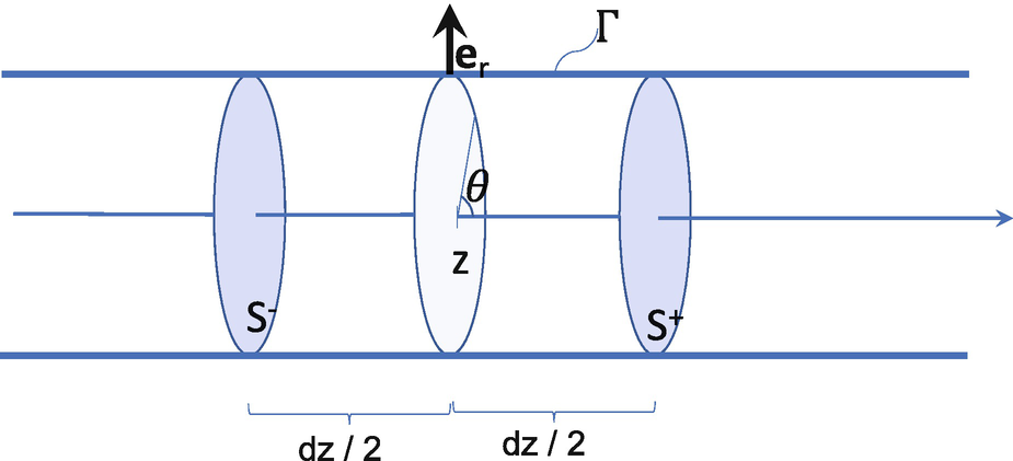
 , see Fig. 2.2. We denote the boundary of V by ∂V = S
−∪ S
+ ∪ Γ, with Γ the part of the boundary of V intercepting the vessel wall. The 1D model is derived by integrating equations (2.3) in V and doing the limit as dz → 0, assuming all quantities are smooth enough.
Portion of the tube between  and
and 
 . Using this expression, the divergence theorem and the mean-value theorem for integrals, we have
 for the continuity equation.
 Due to H2, boundaries S
− and S
+ do not move longitudinally, and due to H6, u
z = 0 on Γ. Thus
  and
and 

 , we obtain
 ![$$\displaystyle \begin{aligned} \begin{array}{rcl} \int_{V} \operatorname{div}(u_z\mathbf{u}) dv &\displaystyle = &\displaystyle \alpha \left[ A\left(z + \frac{dz}{2}\right)\bar{u}^2\left(z +\frac{dz}{2}\right) -A\left(z - \frac{dz}{2}\right)\bar{u}^2\left(z -\frac{dz}{2}\right) \right]\\ &\displaystyle \approx&\displaystyle \alpha\frac{\partial (A\bar{u}^2)}{\partial z} {} \end{array} \end{aligned} $$](../images/475466_1_En_2_Chapter/475466_1_En_2_Chapter_TeX_Equ7.png)

 thus
thus ![$$\displaystyle \begin{aligned} \begin{array}{rcl} \int_{\varGamma} P {\mathbf{n}}_z ds &\displaystyle =&\displaystyle -P(z ) \left(\int_{S^+} ds - \int_{S^-}ds\right) + o(dz) \\ &\displaystyle =&\displaystyle -P(z ) \left[A\left(z +\frac{dz}{2}\right) - A\left(z -\frac{dz}{2}\right)\right] + o(dz) \approx - P(z )\frac{\partial A}{\partial z}(z) \end{array} \end{aligned} $$](../images/475466_1_En_2_Chapter/475466_1_En_2_Chapter_TeX_Equ9.png)

 , we have:
 by assuming that the variation of axial velocity u
z along the axial direction z is small compared to the other terms. From H1 the gradient of u
z becomes
  , and ∇u
z ⋅n becomes
  . Recalling expression (2.2), we have that
  . Noticing that r = R on Γ, we obtain:


 , with E and ξ the Young Modulus and the Poisson ratio of the wall material, and h is the wall thickness. Parameters A
0 and β may vary with z. We define
  , which becomes
  for expression (2.9) and considering A
0 and β constant along z. In this case, system (2.8) can be diagonalized, meaning it is a strictly hyperbolic system of PDEs, describing very well wave propagation phenomenon. Indeed, system (2.8) with (2.9) has two eigenvalues, given by
  . If we choose α = 1, corresponding to a flat profile, we obtain
  . Under physiological conditions, the mechanical properties of blood and of the arterial wall, reflected on c through β, are such that
  , meaning that the two eigenvalues have opposite signs. Indeed, characteristic values of c are of the order of 103m/s [13], while
  is of the order of 101 [14]. This means that system (2.8) describes two waves travelling along the cylindrical vessel, one moving forward and the other backwards.
Let R = [r
1r
2] and L = [l
1l
2] be the matrices of the right and left eigenvectors, respectively, such that LR = I, with I the identity matrix. Then, if there exist quantities W
1 and W
2 such that  and
and  , for U = [A, Q]T, which is the case if α = 1 and K
r = 0 (see for instance [9]), functions W
1 and W
2 are characteristic variables [15]. This means that, up to the additive source term, variables W
i, i = 1, 2 are constant along the characteristic lines, that is, along the lines satisfying the differential equation
  Given the pressure-area relation (2.9) and α = 1, W
1 and W
2 are given by
  .
.
Finally, to completely define problem (2.8), we must provide initial conditions A(0, z) = A 0, Q(0, z) = Q 0 and boundary conditions, which in general can be written as ϕ 1(A(t), Q(t)) = h 1(t), at z = a, and ϕ 2(A(t), Q(t)) = h 2(t), at z = b, where h 1 and h 2 are given functions. The number of boundary conditions to apply at each end is the number of incoming characteristics at that point. Thus, here we must impose exactly one boundary condition at z = a and z = b, respectively [15]. Functions ϕ i, i = 1, 2, produce admissible boundary conditions as long as they do not depend only on the exiting characteristic.
2.3 Numerical Approximation of the 1D Model
The numerical discretization of the 1D hyperbolic model is carried out using the finite element Lax-Wendroff method, [15, 16]. Being a second-order explicit scheme in time, it has excellent dispersion error properties and it is easily implemented.
Being explicit, the stability of the numerical scheme depends on the satisfaction of a CFL type condition (see [9]) relating the time step Δt with the space step h
i: ![$$\varDelta t \leqslant (\sqrt {3}/3) \min _{0 \leqslant i \leqslant N} \left [ \frac {h_{i}}{\max _{k=1,2} \lambda _{k}(z_{i})} \right ]$$](../images/475466_1_En_2_Chapter/475466_1_En_2_Chapter_TeX_IEq33.png) , where z
i, i = 0, …, N, are the mesh nodes, and h
i = z
i+1 − z
i is the measure of the i-th spacial element.
, where z
i, i = 0, …, N, are the mesh nodes, and h
i = z
i+1 − z
i is the measure of the i-th spacial element.
2.3.1 Boundary and Compatibility Conditions for the Discrete Problem

 is obtained following the characteristic line from t = t
n:
  , where x
k is the foot of the characteristic line of W
i at t
n, i = 1, 2.
, where x
k is the foot of the characteristic line of W
i at t
n, i = 1, 2.![$$\displaystyle \begin{aligned} \left[ \begin{array}{cc} \frac{1}{A^{n+1}(a)}\beta\frac{\sqrt{A^{n+1}(a)}-\sqrt{A_0}}{A_0} & 0 \\ -\sqrt{\frac{8\beta}{\rho A_0}}\frac{(A^{n+1}(a))^{1/4}-A_0^{1/4}}{A^{n+1}(a)} & \frac{1}{A^{n+1}(a)} \end{array} \right] \left[ \begin{array}{c} A^{n+1}(a) \\ Q^{n+1}(a) \end{array} \right] = \left[ \begin{array}{c} h_1^{n+1}\\C_{x_a}^{n} \end{array} \right] \end{aligned}$$](../images/475466_1_En_2_Chapter/475466_1_En_2_Chapter_TeX_Equd.png)
 and x
a = a − Δtλ
2(Q
n(a), A
n(a)) is the foot of the exiting characteristic W
2 at z = a. If, at z = b, a condition on the entering characteristic is imposed W
2(t, b) = h
2(t), then the non-linear system to be solved at each time step is
 ![$$\displaystyle \begin{aligned} \left[ \begin{array}{cc} -\sqrt{\frac{8\beta}{\rho A_0}} \frac{(A^{n+1}(b))^{1/4}-A_0^{1/4}}{A^{n+1}(b)} & \frac{1}{A^{n+1}(b)} \\ \sqrt{\frac{8\beta}{\rho A_0}} \frac{(A^{n+1}(b))^{1/4}-A_0^{1/4}}{A^{n+1}(b)} & \frac{1}{A^{n+1}(b)} \end{array} \right] \left[ \begin{array}{c} A^{n+1}(b) \\ Q^{n+1}(b) \end{array} \right] = \left[ \begin{array}{c} h_2^{n+1}\\C_{x_b}^{n} \end{array} \right] \end{aligned}$$](../images/475466_1_En_2_Chapter/475466_1_En_2_Chapter_TeX_Eque.png)
 and x
b = b − Δtλ
1(Q
n(b), A
n(b)) is the foot of the exiting characteristic W
1 at z = b.
and x
b = b − Δtλ
1(Q
n(b), A
n(b)) is the foot of the exiting characteristic W
1 at z = b.Very often the incoming characteristic is put equal to zero at the exiting point, W 2(t, z) = 0, corresponding to an absorbing boundary condition, meaning nothing enters the domain. This fact has been exploit to impose absorbing boundary conditions on 3D FSI models for blood flow [17].
2.3.2 Modular Simulation of Arterial Networks
Coupling single tubes: used to model, for instance, long tubes where physical characteristics vary.
Bifurcation of an artery into two arteries: this is the most common, since almost all arteries enventually bifucarte to carry out blood for the whole body.
Merging of two arteries into one artery: this situation is more rare, occurring for instance with the vertebral arteries (left and right), that merge into the basilar artery before reaching the Circle of Willis at the bottom of the brain.
 , [7, 9].
 , k = a, b, i = 1, 2, 3 are the foot of the outgoing characteristic lines passing in point (k
i, t
n+1). For the bifurcation (b) and merging (m) we have the following systems
2.4 Simulating Anatomical Variations of the Circle of Willis


Representation of the main arteries of the Circle of Willis (CoW)

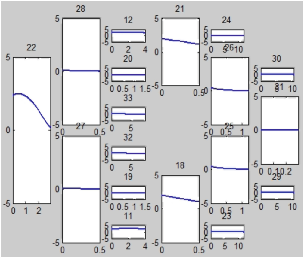
Flow rate [cm3∕s] through the main arteries of the complete CoW at a particular time t

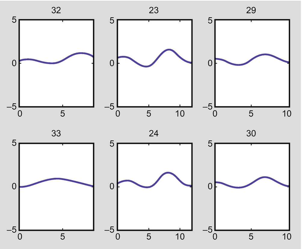
Flow rate when the right posterior cerebral artery is missing (right PCA, artery 28 in Fig. 2.3)

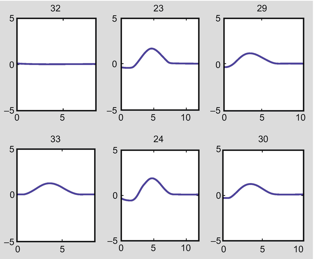
Flow rate in the arteries when both the right posterior communicating artery (PCoA) and the left posterior cerebral artery (PCA) are absent (arteries 20 and 27 in Fig. 2.3)
2.5 Increasing the Complexity of the 1D Model: Including Curvature
The 1D hyperbolic model for blood flow in arteries studied in the previous sections is a simplified model with desirable mathematical properties, namely it is an hyperbolic system of PDEs. It may be considered one of the simplest 1D model for blood pulse. More complex models can be considered by accounting for variations of the radius or the wall properties along z, which introduce derivatives of the parameters A 0 and β, to be included on the source term. Also, more sophisticated pressure-area relations can be used, leading to the appearance of higher order derivatives. These derivatives alter the characteristic of the differential problem, making the numerical treatment and the identification of proper boundary conditions more problematic [9]. These effects also imply the inclusion of new parameters for which it is often difficult to obtain reasonable values.

 , with a∕2 = Q∕A. In this case, the 3D Navier-Stokes system (2.3) has two extra equations, related to u
x and u
y:
 , we have:
 is the outward unitary normal. Thus
 , then
 , then
  . Since
  on S, we have

 and that

 and hence
  . Finally, for the diffusive term on x, we may neglect
  , obtaining
 we get

 . The resulting 1D system of equations is
 . In this case, two extra equations are needed, for the added quantities b and c, related with the axial velocity profile. These equations are obtained by integrating over the cross section the third equation of (2.11) multiplied by x and y, respectively. Using the same approach and arguments as before, the 1D model in this case becomes:
 , as before, and
  and
and  . This system of PDE’s is significantly more complex than the usual 1D model (2.8). Its mathematical and numerical analysis becomes extremely cumbersome, since many of the nice mathematical characteristics of system (2.8) are lost. Being simplified models, the usefulness o such complex 1D models is questionable. If we need more detail and the cost is such an increase in model complexity, than possibly the best is to use full detailed 3D models.
2.6 Conclusions
One dimensional models for blood flow in arteries are simplified and computationally low cost models, obtained by making simplifying assumptions and performing averaging procedures on the 3D FSI model. The simplest 1D model is described by an hyperbolic system of PDE’s. Despite having a lower level of accuracy compared to the full 3D representation, it captures very effectively the pulsation of blood flow. More complex 1D models can be obtained by relaxation of some simplifying hypothesis, as for instance accounting for curvature. In these cases the 1D mathematical model becomes significantly more complex, losing some of the appealing mathematical properties of the simpler straight tube 1D model. Namely, it is no longer hyperbolic. Being simplified models, the extra complexity introduced in these cases is hardly justified. Except for very particular cases, in general when high accuracy on the blood flow solution is required, 3D FSI full mathematical models tend to be preferable.