3.1 Introduction
- 1.
Visualization of the available kinetics data and calculation of the f original uncertainty parameters of the investigated rate coefficient in selected temperature points.
- 2.
Calculation of the f extreme uncertainty parameters in selected temperature points.
- 3.
Determination of a continuous, temperature dependent uncertainty function
 , which is consistent with the rate coefficient-temperature function.
3.2 Calculation of the Uncertainty Parameters f original in Selected Temperature Points

 and ε := E∕R, the linearized form of the modified Arrhenius equation is

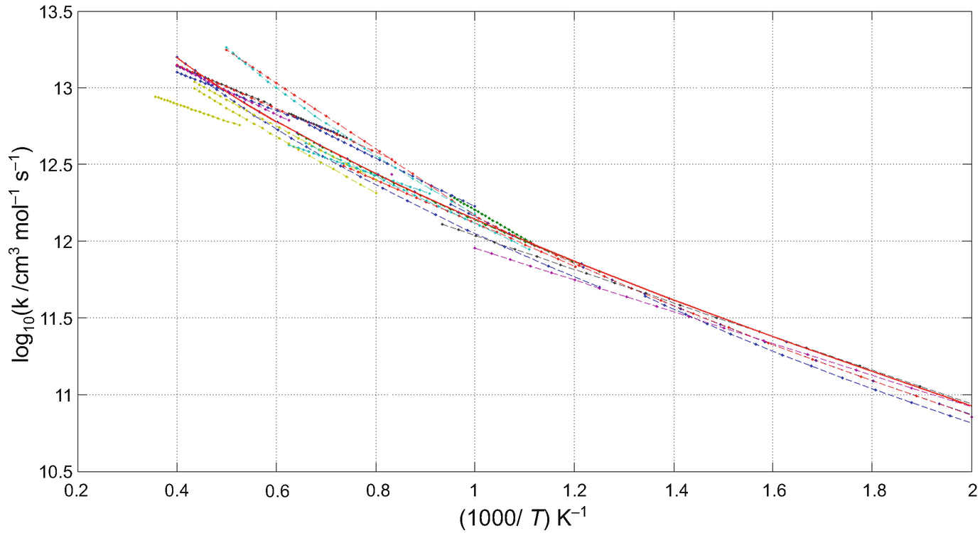
The logarithm of measured and theoretically determined rate coefficients as a function of the reciprocal of temperature belonging to reaction OH+H2=H2O+H
The rate coefficient of an elementary reaction can be determined by various experimental methods. If several measurements were carried out in different laboratories (maybe using different methods) at similar temperatures, then the uncertainty of the rate coefficient can be well assessed at a given temperature or in a narrow temperature interval. If the uncertainty of a rate coefficient is determined from literature data at different temperatures, then these uncertainties can be very different from each other even at nearby temperatures. However, since the measured rate coefficients are interrelated by a common Arrhenius expression, therefore the uncertainties determined at different temperatures are also related. Taking into account the temperature dependence of the rate coefficient, the uncertainty at a given temperature cannot be high if it is low at nearby temperatures.
The next pages discuss the determination of an Arrhenius-equation-consistent uncertainty function from the uncertainties of a rate coefficient valid at given temperatures (or in given temperature intervals) and the features of the corresponding uncertainty domain of the Arrhenius parameters.
 is defined by Baulch et al. [6]:
This definition of uncertainty is related to the limits and does not necessarily have a probabilistic inference. According to Eq. (3.3), the upper and lower extreme values differ from the recommended value by a multiplication factor, which means that, on a logarithmic scale, the extreme values are located symmetrically around the recommended value. The uncertainty bounds for rate coefficient k can be converted to the uncertainty bounds of  .
.
The uncertainty bound of the logarithm of the rate coefficient, κ(T), is ![$$\left [\kappa (T)-\frac {f(T)}{\ln 10} ,\kappa (T)+\frac {f(T)}{\ln 10} \right ]$$](../images/475466_1_En_3_Chapter/475466_1_En_3_Chapter_TeX_IEq5.png) .
.
Our aim is to define a temperature dependent uncertainty function f(T), and thus defining a symmetrical bound for the recommended rate coefficient κ 0(T). This bound will indicate the extreme, but physically realistic rate coefficient values at every temperature.

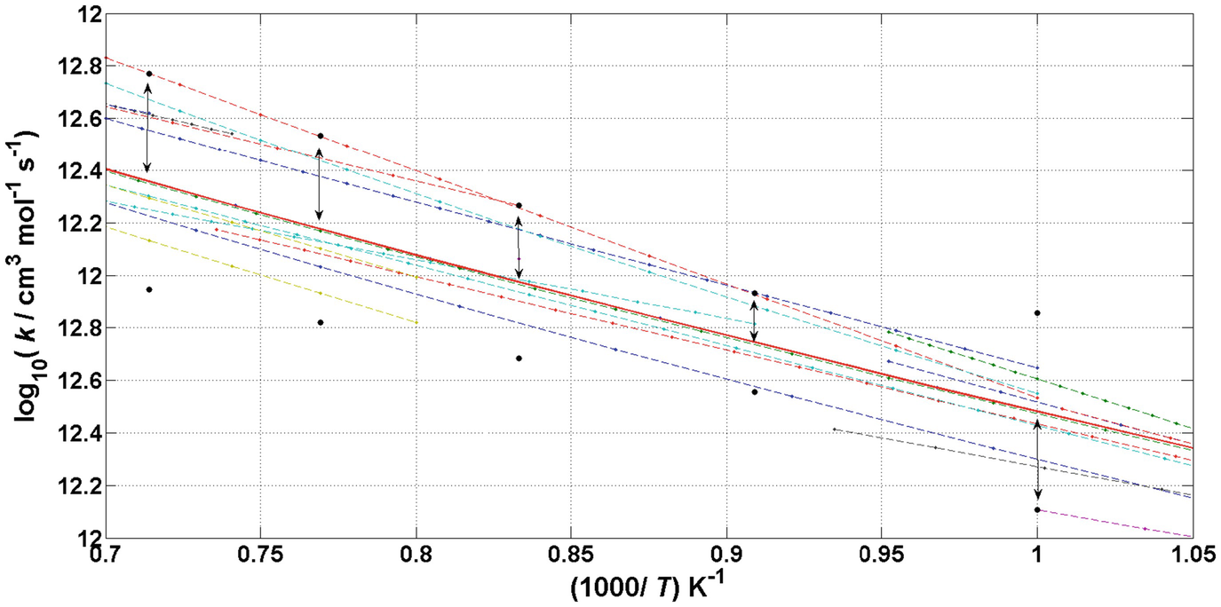
 values for reaction OH+H2=H2O+H at T = 1000, 1100, 1200 and 1300 K. The investigated measurements and theoretical calculations for the values of the Arrhenius parameters and the corresponding temperature intervals are available in the Supplementary Material of [2].
The figure shows the Arrhenius curves of the rate coefficients that had been presented in Fig. 3.1, now in a narrower temperature interval (dashed lines). The mean value of the rate coefficient of reaction OH+H2=H2O+H was added (solid red line in the middle). The black circles and the sections with arrowheads (↔) show the extent of the  values at T = 1000, 1100, 1200 and 1300 K
Chemical kinetic databases contain suggested values of Arrhenius parameters A, n, E (or transformed Arrhenius parameters α, n, ε) and the temperature range where these values are relevant. Such information is available from the NIST Chemical Kinetics Database [7], the evaluations of Warnatz [8], Tsang et al. (see e.g. [9–11]), Baulch et al. (see e.g.[6, 12, 13]) and the review of Konnov [14].
Collect all suggested values for the rate coefficient of reaction H+O2=O+OH and create a user-friendly program code to visualize them in an Arrhenius plot. Using Arrhenius parameters A = 2.07E+14 cm3mol−1s−1, n = −0.097,  K (the mean rate expression recommended by Baulch et al. [6]), calculate uncertainty parameter
  at temperature points T = 800, 900, …, 2700 K based on Eq. (3.4).
3.3 Calculation of the Uncertainty Values f extreme at Selected Temperature Points
After the calculation of the  point pairs, it is a natural idea fitting a polynomial to these points and using the fitted curve as a temperature dependent uncertainty function. However, the uncertainty bound defined by this function may contain physically not meaningful values of the rate coefficient. For this reason, a refined approach for the determination of the temperature-uncertainty point pairs is needed to obtain a physically relevant bound.
The procedure described here determines the uncertainty domain of Arrhenius parameters (p = (α, n, ε)T) from the uncertainty information for the rate coefficients. In several cases the temperature dependence of the rate coefficient can be described by two Arrhenius parameters (α, ε) or (α, n). In this case the third Arrhenius parameter is set to zero.
 . It is possible to generate all Arrhenius curves κ(T, p) that lie between the uncertainty limits, fulfilling the following 2n
T inequalities:
 , since Arrhenius equation (3.2) is a linear function of parameters α, n, ε, and equation (3.3) defines symmetric linear constraints. A systematic procedure is proposed here for determining the extreme Arrhenius curves, which touch either the lower or the upper uncertainty limit at least at 2 or 3 temperatures for the 2- and the 3-parameter cases, respectively, and also go within the upper and lower uncertainty limits at all other temperatures. Formally, these criteria correspond to Arrhenius functions that fulfil at least 2 or 3 equality relations in Eqs. (3.5) and for the remaining 2n
T − 2 or 2n
T − 3 cases, respectively, either the equality or the inequality is fulfilled. The minimum and maximum values of these curves at a given temperature define the edges of the band of all possible Arrhenius curves.
 usually has a smaller contribution to the temperature dependence of the rate coefficient than − ε∕T, since
  changes more slowly than 1∕T at combustion temperatures (800 K–2700 K). The effect of a change in the temperature exponent n on the rate coefficient at high temperatures can be well compensated by adjusting the pre-exponential factor α, leading to a very strong anti-correlation between α and n in most determinations. This implies that values of n, which significantly deviate (i.e. by ± 10) from the central n
0, can also fulfil all the inequality requirements in Eq. (3.5) if the initial uncertainty limits are not too tight. Both theoretical considerations [15] and the typical range of values of n in kinetic databases [7] show that the temperature exponent n of elementary chemical reactions should take values of small negative or positive numbers. Therefore, we recommend confining the range of n values to a narrow (i.e. Δn = 2) symmetric interval around the central value n
0 when the band of possible Arrhenius curves is determined through finding extreme Arrhenius curves.
 curve. These new limits, obtained from a set of uncertainty values f and a user-defined Δn, uniquely define a new, continuous uncertainty function
  :
: 
 is always less than or equal to the original uncertainty
  , at every temperature T
i (i = 1, .., n
T).
, at every temperature T
i (i = 1, .., n
T).Create a program code to calculate  uncertainty values at temperature points T = 800, 900, …, 2700 K based on the calculated
  points for elementary reaction H+O2=O+OH.
3.4 Calculation of Uncertainty Function 

If the rate coefficients are considered as random variables, then Arrhenius parameters α, n and ε are also random variables, since these can be calculated from the random values of κ(T) at three given temperatures using the linearized Arrhenius equation (Eq. (3.2)). The joint probability density function of the Arrhenius parameters is independent of temperature. This means that all central moments are also independent of temperature, including their expected values ( ), variances
  and correlations
  .
.

A method was proposed [1] for the determination of the covariance matrix of the Arrhenius parameters using Eqs. (3.8) and (3.9) from uncertainty parameter f of the rate coefficient at various temperatures. To determine the elements of the covariance matrix for the three-parameter Arrhenius expression, the uncertainty of the rate coefficient ( ) has to be known at least at six different temperatures. In the (α, ε) and (α, n) two-parameter cases, the uncertainty of the corresponding Arrhenius parameters can be handled in a similar way and the uncertainty of the rate coefficient has to be known at least at three temperatures [1]. Having calculated the
  values at temperature points T
i, the
  values are also available. The four or six elements of the covariance matrix have to be determined by minimising the difference between the values
  and
and  for all T
i, (i = 1, …, n
T).
Equations (3.8) and (3.9) provide a means for storing the  function in the form of the covariance matrix of Arrhenius parameters. The uncertainty parameter temperature function calculated from the covariance matrix can be used as a first guess (prior) and conservative estimation of the uncertainty of a rate coefficient and it can be used as a starting point of a more refined estimation [25] of the temperature dependent uncertainty of the rate coefficient.
The uncertainty function reconstructed from the covariance matrix is called prior uncertainty and denoted as  .
.
In Eq. (3.8), the parameter μ defines the proportionality between the uncertainty parameter f and the standard deviation σ κ. When the uncertainty f prior is calculated via σ κ from the covariance matrix Σ p, the same parameter μ has to be used. This means that the value of μ is arbitrary in the storage of the f values in the covariance matrix, and the only important assumption here is that the uncertainty parameter f is proportional to the standard deviation of κ.
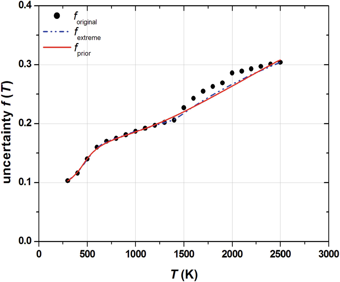
 ) values and the calculated
  function for reaction OH+H2=H2O+H. The red solid line in Fig. 3.3 represents the
 function, which was fitted to points
  ), where T
i = 300 K, 400 K,…, 2500 K.
The calculated f
original(T
i) values (black circles), the extreme uncertainty function,  (blue dashed line) and the fitted f
prior(T) function (red solid line) for reaction OH+H2=H2O+H at temperature points T = 300 K, 400 K, …, 2500 K
Project no. ED_18-1-2019-0030 (Application-specific highly reliable IT solutions) has been implemented with the support provided from the National Research, Development and Innovation Fund of Hungary, financed under the Thematic Excellence Programme funding scheme.
