7.1 Introduction
Modeling the heating of an object is an important task in many applicational problems. Moreover, a matter of particular interest is to find the optimal heating of an object such that it has a desired temperature distribution after some given time. In order to formulate such optimal control problems and to solve them, a cost functional subject to a time-dependent partial differential equation (PDE) is derived. One of the profound works paving the way for PDE-constrained optimization’s relevance in research and application during the last couple of decades is Lion’s work [9] from 1971. Some recent published monographs discussing PDE-constrained optimization as well as various efficient computational methods for solving them are, e.g., [1, 6], and [11], where the latter one is used as basis for the discussion on solving the optimal heating problem of this work.
The goal of this work is to derive a simple mathematical model for finding the optimal heating of the air in a glass dome represented by a half sphere, where a swimming pool is located in the bottom of the dome and the heat sources (or heaters) are situated on a part of the boundary of the glass dome. The process from the model to the final numerical simulations usually involves several steps. The main steps in this work are the setting up of the mathematical model for the physical problem, obtaining some analytical results of the problem, presenting a proper discretization for the continuous problem and finally computing the numerical solution of the problem. The parabolic optimal control problem is discretized by the finite element method in space, and in time, we use the implicit Euler method for performing the time stepping. The used solution algorithm for the discretized problem is the projected gradient method, which is for instance applied in [5] as well as in more detail discussed in [4, 6, 8, 10].
We want to emphasize that the model and the presented optimization methods for the heating process of this work are only one example for a possible modeling and solution. In fact, the stated model problem has potential for many modeling tasks for students and researchers. For instance, different material parameters for the dome as well as for air and water could be studied more carefully. The optimal modeling of the heat sources could be stated as a shape optimization problem or instead of optimizing the temperature of the air in the glass dome, one could optimize the water temperature. This would correspond to a final desired temperature distribution corresponding to the boundary of the glass dome, where the swimming pool is located, for the optimal control problem. Another task for the students could be to compute many simulations with, e.g., Matlab’s pdeModeler to derive a better understanding of the problem in the pre-phase of studying the problem of this work. However, we only want to mention here a few other possibilities for modeling, studying and solving an optimal heating problem amongst many other tasks, and we are not focusing on them in the work presented here.
This article is organized as follows: First, the model of the heating process is formulated in Sect. 7.2. Next, Sect. 7.3 introduces the optimal control problem, which describes the optimal heating of the glass dome such that the desired temperature distribution is attained after a given time. In Sect. 7.4, proper function spaces are presented in order to discuss existence and uniqueness of the optimal control problem. We derive the reduced optimization problem in Sect. 7.5 before discussing its discretization and the numerical method for solving it, the projected gradient method, in more detail in Sect. 7.6. Numerical results are presented as well as conclusions are drawn in final Sect. 7.7.
7.2 Modeling
This section presents the modeling process. The physical problem is described in terms of mathematical language, which includes formulating an initial version of the problem, but then simplifying it in order to derive a version of the problem which is easier to solve. However, at the same time, the problem has to be kept accurate enough in order to compute an approximate solution being close enough to the original solution. That is exactly one of the major goals of mathematical modeling. In the following, we introduce the domain describing the glass dome, where an indoor swimming pool is located in the bottom of the dome, and the position of the heaters. The concrete equations describing the process of heating and the cost functional subject to them modeling the optimization task are discussed in next Sect. 7.3.
We have an indoor swimming pool which is located under a glass dome. For simplicity, it is assumed that we have an isolated system in the glass dome, so no heat can leak from the domain. The swimming pool covers the floor of the glass dome and we assume that the heaters are placed next to the floor up on the glass all around the dome. The target of the minimization functional is to reach a desired temperature distribution at the end of a given time interval (0, T), where T > 0 denotes the final time, with the least possible cost.
 is a bounded Lipschitz domain. We subdivide its boundary Γ into four parts: the glass part Γ
1, the floor which is the swimming pool Γ
2 and the heaters Γ
3 and Γ
4. The domain Ω and its boundaries are illustrated in Fig. 7.1.
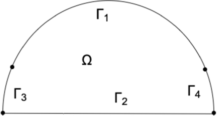
The domain Ω reduced from 3d to 2d due to symmetry properties describing the glass dome and its heaters placed at the ground of the glass dome next to the floor, hence subdividing the boundary Γ = ∂Ω into four parts Γ 1, Γ 2, Γ 3 and Γ 4
7.3 Optimal Control Problem
In this section, the optimal control problem is formulated, where an optimal control function u has to be obtained corresponding to the heating of the heat sources on the boundary Γ R := Γ 3 ∪ Γ 4 such that the state y reaches a desired temperature distribution y d after a given time T. This problem can be formulated in terms of a PDE-constrained optimization problem, which means minimizing a cost functional subject to a PDE and with u being the control function.


The goal is to find the optimal set of state and control (y, u) such that the cost is minimal.
7.4 Existence and Uniqueness
In this section, we discuss some basic results on the existence and uniqueness of the parabolic initial-boundary value problem (7.2)–(7.6), whereas we exclude the details. They can be found in [11]. We first introduce proper function spaces leading to a setting, where existence and uniqueness of the solution can be proved.
 is defined as follows

For the model problem of this work, the dimension is d = 2. In the following, let {V, ∥⋅∥V} be a real Banach space. More precisely, we will consider V = H 1(Ω) in this work.


The relation V ⊂ H = H ∗⊂ V ∗ is called a Gelfand or evolution triple and describes a chain of dense and continuous embeddings.
 for a given u ∈ U
ad. Moreover, the solution depends continuously on the data, which means that there exists a constant c > 0 being independent of u, g and y
0 such that
 ![$$\displaystyle \begin{aligned} \max_{t \in [0,T]} \|y(\cdot,t)\|{}_{L^2(\varOmega)} + \|y\|{}_{W^{1,0}_2(Q_T)} \leq c (\|u\|{}_{L^2(\varSigma_R)} + \|g\|{}_{L^2(\varSigma_2)} + \|y_0\|{}_{L^2(\varOmega)}) \end{aligned} $$](../images/475466_1_En_7_Chapter/475466_1_En_7_Chapter_TeX_Equ14.png)
 . Furthermore, since
  and it is a weak solution of problem (7.2)–(7.6), y also belongs to W(0, T). The following estimate holds:
 being independent of u, g and y
0. Hence, problem (7.2)–(7.6) is also well-posed in the space W(0, T).
being independent of u, g and y
0. Hence, problem (7.2)–(7.6) is also well-posed in the space W(0, T).Note that the Neumann boundary conditions on Γ 1 are included in both estimates (7.14) and (7.15) related to the well-posedness of the problem (as discussed in [11]). However, the Neumann boundary conditions (7.3) are equal to zero.
Under the assumptions that  is a bounded Lipschitz domain with boundary Γ, λ ≥ 0 is a fixed constant, y
d ∈ L
2(Q
T), α, β ∈ L
∞(Σ
R), and u
a, u
b ∈ L
2(Σ
R) with u
a ≤ u
b a.e. on Σ
R, together with the existence and uniqueness result on the parabolic initial-boundary value problem (7.2)–(7.6) in W(0, T), the optimal control problem (7.1)–(7.7) has at least one optimal control
  . In case of λ > 0 the optimal control
  is uniquely determined.
7.5 Reduced Optimization Problem
In order to solve the optimal control problem (7.1)–(7.7), we derive the so called reduced optimization problem first.

 has to be calculated by deriving the adjoint problem which is given by


 is given by
 denoting the characteristic function on Γ
R. The projected gradient method can be now applied for computing the solution of the PDE-constrained optimization problem (7.1)–(7.7). We denote by
 ![$$\displaystyle \begin{aligned} \mathcal{P}_{[u_a,u_b]}(u) = \max\{u_a, \min\{u_b,u\}\} \end{aligned} $$](../images/475466_1_En_7_Chapter/475466_1_En_7_Chapter_TeX_Equ23.png)
Now putting everything together, the optimality system for (7.1)–(7.7) and a given λ > 0 reads as follows
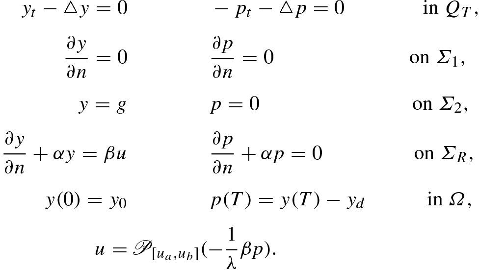

In case that there are no control constraints imposed, the projection formula simplifies to u = −λ −1βp.
7.6 Discretization and Numerical Method
In order to numerically solve the optimal control problem (7.1)–(7.7), which is equivalent to solving (7.24), we discretize the heat equation in space by the finite element method and in time. We use the implicit Euler method for performing the time stepping.
 to construct the finite element space V
h. For more information, we refer the reader to [3] as well as to the newer publications [2, 7]. Discretizing problem (7.24) by computing its weak formulations and then inserting the finite element approximations for discretizing in space leads to the following discrete formulation:

![$$\displaystyle \begin{aligned} \underline{u}_h = \mathcal{P}_{[u_a,u_b]}(-\frac{1}{\lambda} \beta \underline{p}_h) \end{aligned} $$](../images/475466_1_En_7_Chapter/475466_1_En_7_Chapter_TeX_Equ28.png)

 ,
,  and
and  . The values for
  are set to g in the nodal values on the boundary Γ
2 and the problems are solved only for the degrees of freedom. The matrices M
h,
  and K
h denote the mass matrix, the mass matrix corresponding only to the Robin boundary Γ
R and the stiffness matrix, respectively. The entries of the mass and stiffness matrices are defined by the integrals
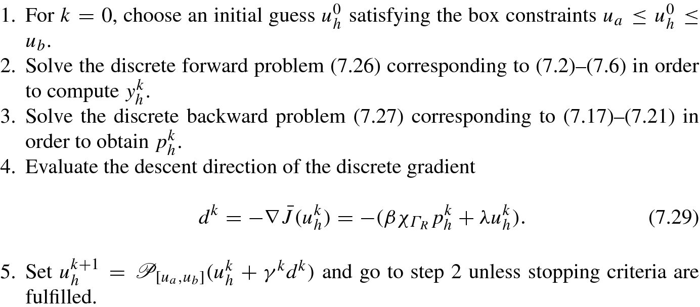
For a first implementation, the step length γ = γ k can be chosen constant for all k. However, a better performance is achieved by applying a line search strategy as for instance the Armijo or Wolfe conditions to obtain the best possible γ k in every iteration step k. We refer the reader to the methods discussed for instance in [5]. However, these strategies are not subject to the present work.
7.7 Numerical Results and Conclusions
In this section, we present numerical results for solving the type of model optimization problem discussed in this article and draw some conclusions in the end. The numerical experiments were computed in Matlab. The meshes were precomputed with Matlab’s pdeModeler. The finite element approximation and time stepping as well as the projected gradient algorithm were implemented according to the discussions in the previous two sections.

The nodes marked corresponding to different boundaries and the interior of the domain Ω on a mesh with 4073 nodes
In the numerical experiments, we choose the following given data: the water temperature g = 20, the parameters α = β = 102, the final time T = 1, the box constraints u
a = 20 and u
b = 60, the desired final temperature y
d = 30 and the initial value y
0 = 0 satisfying the boundary conditions. For the step lengths γ
k of the projected gradient algorithm, we choose the golden ratio γ
k = γ = 1.618 constant for all iteration steps k. The stopping criteria include that the norm of the errors  or |e
k+1 − e
k| < 𝜖
2 with 𝜖
1 = 10−1 and 𝜖
2 = 10−2 have to be fulfilled as well as setting a maximum number of iteration steps k
max = 20 with k < k
max.
Number of iterations needed to satisfy the stopping criteria for different mesh sizes and numbers of time steps for a fixed cost coefficient λ = 10−2
Mesh size | Time steps | Iteration steps |
|---|---|---|
76 | 125 | 7 |
275 | 250 | 5 |
1045 | 1000 | 19 |
4073 | 4000 | 19 |
16,081 | 16,000 | 4 |
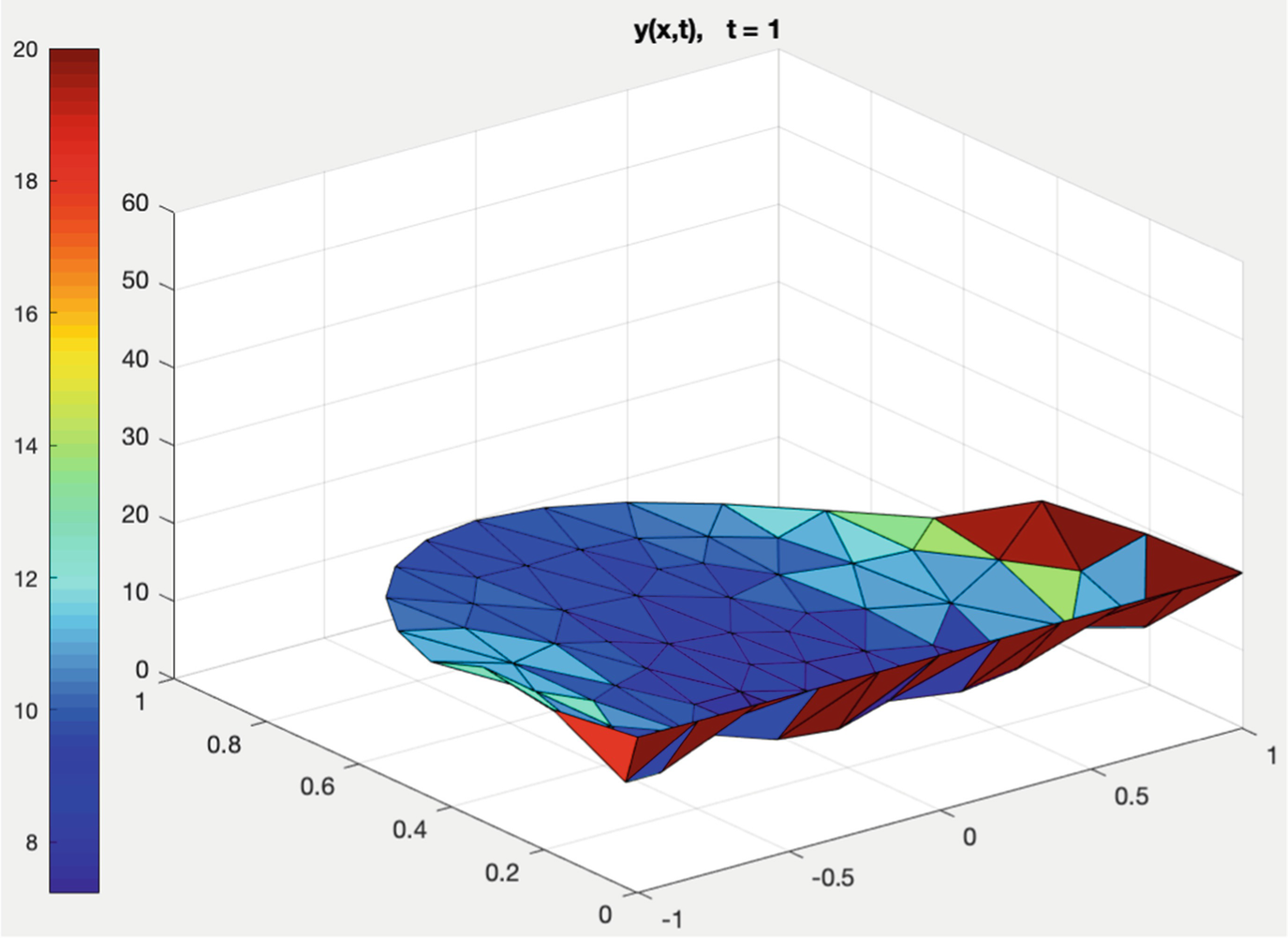
The approximate solution y for final time t = T = 1 on a mesh with 76 nodes
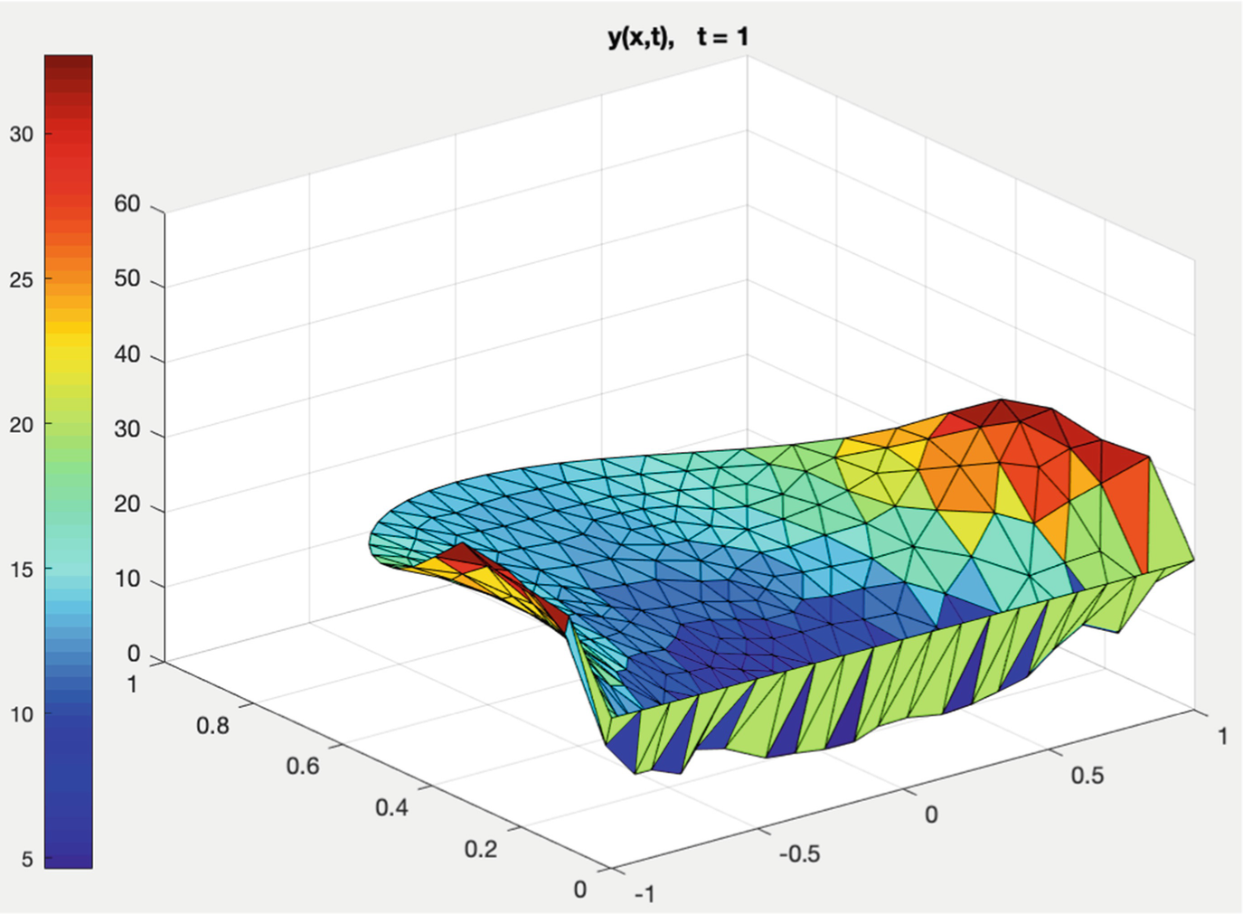
The approximate solution y for final time t = T = 1 on a mesh with 275 nodes

The approximate solution y for final time t = T = 1 on a mesh with 1045 nodes
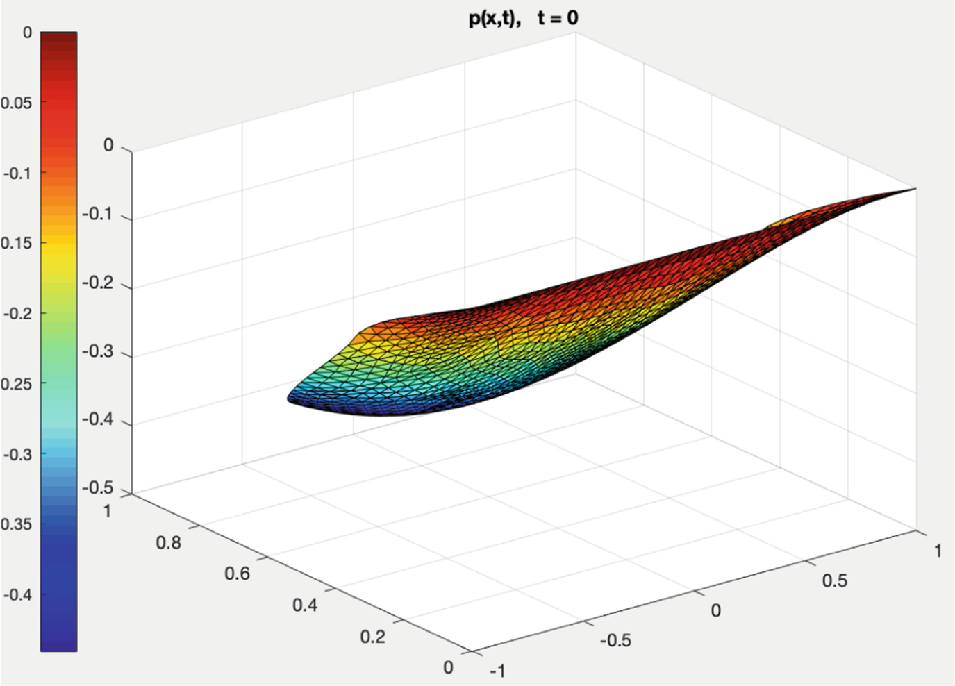
The approximate adjoint state p for time t = 0 on a mesh with 1045 nodes
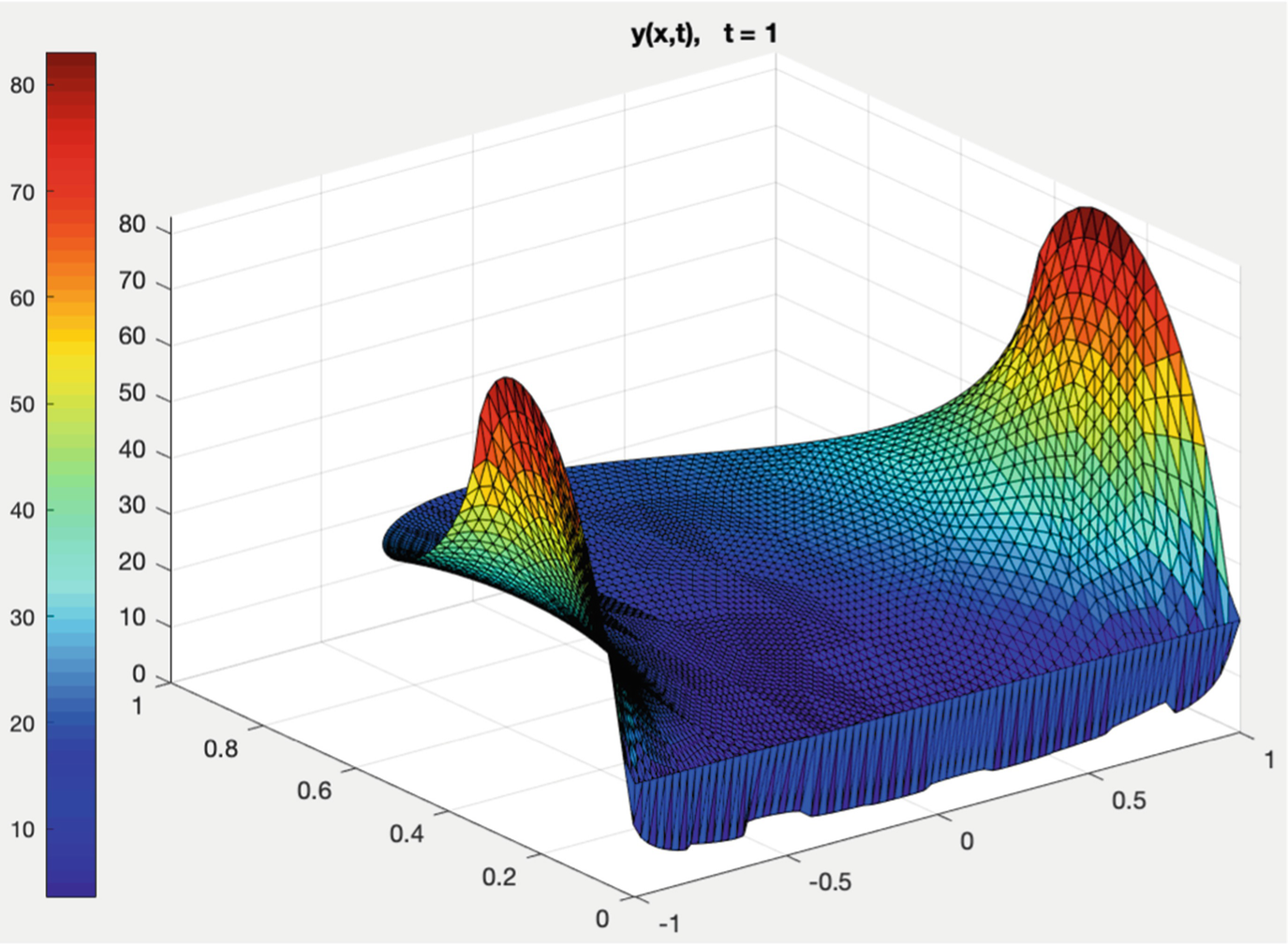
The approximate solution y for final time t = T = 1 on a mesh with 4073 nodes

The approximate solution y for final time t = T = 1 on a mesh with 16,081 nodes
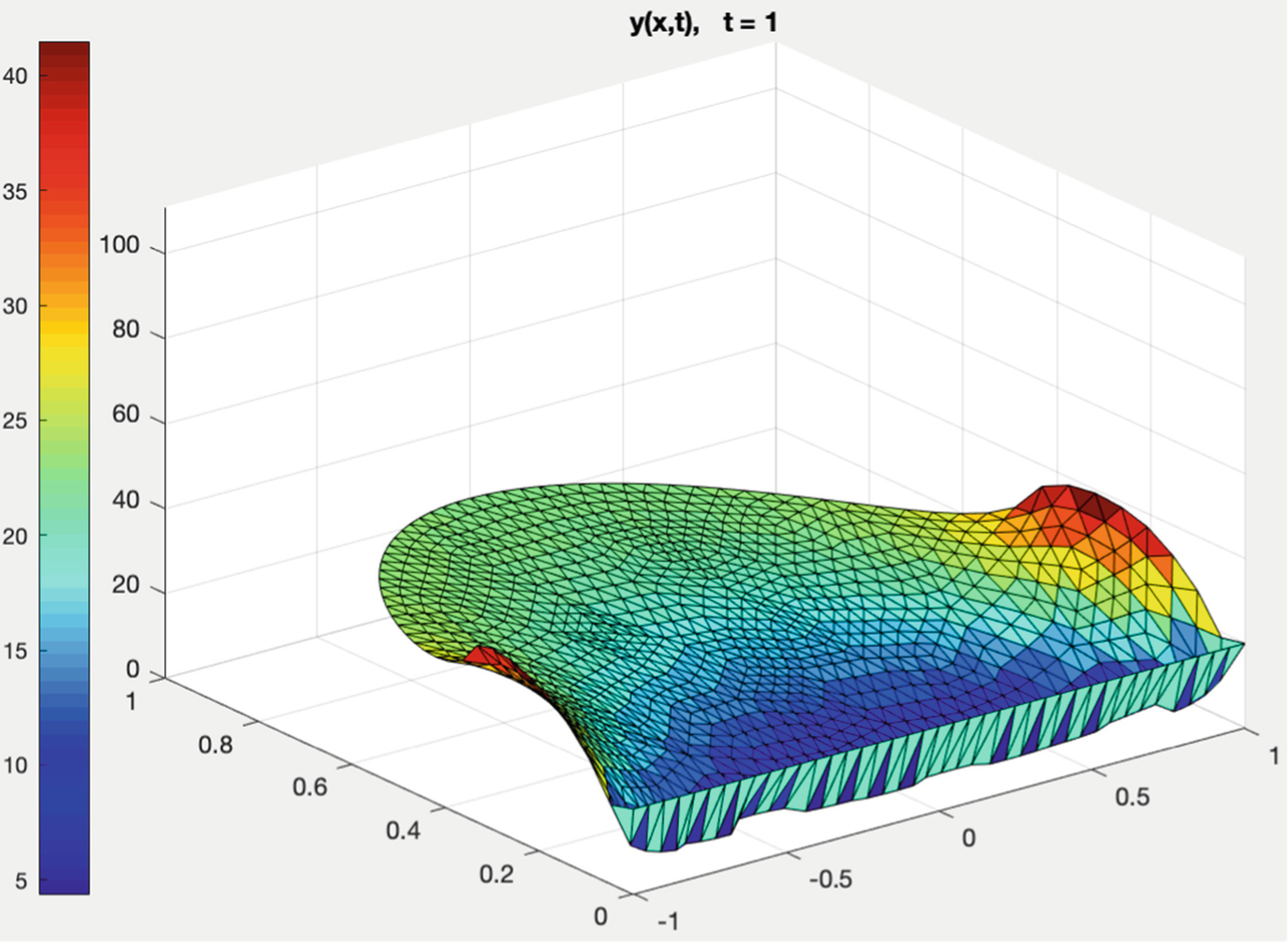
The approximate solution y for final time t = T = 1 on a mesh with 1045 nodes for the value λ = 10−4
Number of iterations needed to satisfy the stopping criteria for different cost coefficients λ ∈{10−4, 10−2, 1, 102, 104} on grids with mesh sizes n = 275 and n = 1045 with 250 and 1000 time steps, respectively
λ | Iteration steps (275/250) | Iteration steps (1045/1000) |
|---|---|---|
10−4 | 5 | 19 |
10−2 | 5 | 19 |
1 | 7 | 19 |
102 | 4 | 4 |
104 | 4 | 4 |
The results of Tables 7.1 and 7.2 were included as example how one can perform different tables for different parameter values or combinations. Students or researchers could compute exactly these different kinds of numerical experiments in order to study the practical performance of the optimization problem.
After presenting the numerical results, we have to mention again that the step length γ = γ k of the projected gradient method has been chosen constant for all k in all computations. However, better results should be achieved by applying a suitable line search strategy, see Remark 7.2. With this we want to conclude that the optimal control problem discussed in this work is one model formulation for solving the optimization of heating a domain such as the air of a swimming pool area surrounded by a glass dome. Modeling and solving the optimal heating of a swimming pool area has potential for many different formulations related to mathematical modeling, discussing different solution methods and performing many numerical tests including “playing around” with different values for the parameters, constants and given functions, and finally choosing proper ones for the model problem. All of these tasks can be performed by students depending also on their previous knowledge, interests and ideas.
I would like to thank my students T. Bazlyankov, T. Briffard, G. Krzyzanowski, P.-O. Maisonneuve and C. Neßler for their work at the 26th ECMI Modelling Week which provided part of the starting point for this work. I gratefully acknowledge the financial support by the Academy of Finland under the grant 295897.