Design of passive solar architecture is more complex than that of a traditional modern building. The sun’s path in relation to the site is dynamic. Air-flow in relation to the site is irregular and at times turbulent. The interior temperature is chaotic within limits of the comfort zone which is determined as much by culture and social mores as scientific measurement.
Until sophisticated computer simulation became available, prediction of performance was very difficult because of the multiple variables involved. Even the economics of green building is best described by a fractal.
Passive solar architecture embraces this complexity to develop architecture that is more wholistic and less of an abstraction.
Passive solar design relies on an intimate feeling for sun locations at any time, day or month. For detailed isogenic maps of N. America, S. America, Europe, Middle East, Orient/ New Guinea, Australia and New Zealand visit: http://www.geo-orbit.org/sizepgs/magmapsp.html
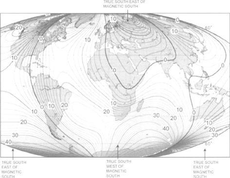
Use the magnetic declination map above and the sun path diagrams on the following pages to understand the sun- earth - site - time relationship.
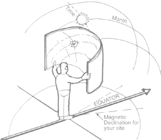
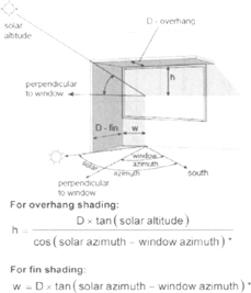
Using the preceding sun path charts, you can calculate for sun and shade as shown to the right. This is good for specific details, but for the whole building it is often easier to create a digital or physical model. Physical models can utilize the sun-dial device called a sun peg diagram. The following sun peg charts will show the exact position of sunlight and shadow on a model of any scale, on any date, at any time of day between shortly after sunrise and shortly before sunset.
1. Find the chart nearest your latitude.
2. Make a copy of the chart.
3. Construct a peg whose finished height above the chart surface corresponds to the “peg height” shown on your copy of the chart. This peg must stand perfectly vertical relative to the model.
4. Mount your copy of the chart on the model to be tested. The chart must be perfectly horizontal over its entire surface, and the true north or south arrow must correspond exactly to true north or south on the model.
5. Mount your vertical peg at the location shown on the chart.
6. Choose a test time and date. Take your model out into direct sunlight.
Then tilt the model until the shadow of the peg points toward the intersection of the chosen time’s line and the chosen date’s curve. When the end of the peg’s shadow touches this intersection, your model will show the same sun-shadow patterns as would occur on the time and date of the intersection you chose. [46]
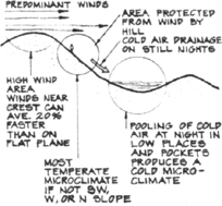
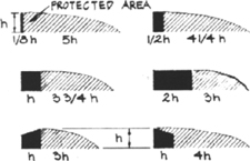
Besides site selection, wind protection may be provided by adjacent buildings, walls or vegetation. Generally, the thinner the adjacent element, the larger the protected area down wind.
For a typical house, heat loss by air infiltration can be 2 ½ times as great in a 2.2 m/s [5 mph] wind verses no wind. Since infiltration may account for up to half of the building’s heating load, protection from wind can produce a considerable reduction in heating requirements.
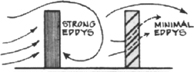
Solid windbreaks produce strong eddy currents which negate much of their effectiveness. A slatted fence prevents this.

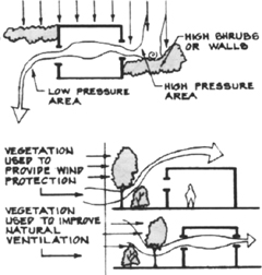
Thick vegetation is highly effective, especially a combination of trees and shrubs as shown.
Trees, shrubs, walls, etc. can often be used to improve natural ventilation even if the building cannot be optimally oriented to the wind.
If windows are on opposite sides, the room should be oriented askew to the wind direction. If the windows are on adjacent walls, the room should be oriented to face directly into the wind.

Height difference between inlet and outlet helps induce natural ventilation during still times.
Air patterns in a room are largely determined by the inlet location and its relationship to the exterior surfaces of the building.
It is important for night vent cooling to wash thermal masses with cool night air via the technique shown.
The same principles apply to the vertical dimension.

Overhangs can have the same effect as wing walls and other barriers in the horizontal dimension.
Outlet size in relation to inlet size largely determines the speed of interior airflow. Change in direction causes greater spread but less speed.
Solar architecture/ passive solar building simulation programs
Since their inception there has been a rapid increase in the number of available building energy simulation programs. Their capabilities have been improving in pace with available computer speed and capacity, allowing ever more detailed aspects of the buildings and their environmental driving forces to be incorporated in the programs. In turn, causing a flourishing of building research to better understand and characterize the important physical processes involved. Focused mainly on residential and small commercial applications, the general capabilities of available programs are listed below.
General purpose programs
These are characterized by their accuracy and extent of options and level of detail, and are generally engineering research oriented. They are mainly used by architects and engineers experienced in simulation and building science. These programs have the following capabilities:
• Transient heat flow in lightweight and heavy mass buildings, usually with a one-dimensional time-domain analysis. Most have transient slab-on-grade heat transfer algorithms, but frequently of limited sophistication.
• Weather tape driven state-of-the-art solar and environmental algorithms.
• Determine heating and cooling loads, and building and environment temperature and heat flow histories.
• State-of-the-art window analysis algorithms, incorporating longwave and short-wave and convective window heat transfers algorithms. Shading and internal solar distribution algorithms are of varied sophistication.
• Separate radiant and convection heat transfer algorithms, although some are limited to a combined coefficient analysis.
• Infiltration and natural ventilation algorithms, with a large variation is algorithm sophistication, a few incorporating inter-zone air flow analysis.
• HVAC system model sophistication varies from simple residential system models to a multitude of commercial building HVAC variants.
• Most have multi-zone modeling capabilities.
• Building geometry is typically specified with text input, but in some cases can be defined using CAD tools.
• Daylight utilization analysis algorithms are common, usually for a limited range of geometries.
• Graphical input and output interfaces are common but not universal.
• Many programs incorporate photovoltaic and life cycle cost analysis.
Variants of programs in this category of programs are frequently used for confirming building compliance with performance based energy standards, in which case some inputs and features are constrained to inputs and features allowed by the standards.
Architectural design oriented programs
Although the general purpose programs are frequently used for architectural design, they have the reputation of being difficult to learn and interpret, time consuming in their detail, and as a result have had a relatively small penetration into the architectural design arena. The more designer friendly architectural design oriented programs are characterized by ease of use, fast running speeds, extensive libraries, easily interpretable graphical input and output, and the ability to integrate simulation into the various phases of the recursive design process. Since many of these are modified versions of general purpose programs, they tend to show their engineering roots.
Educational variants of the architectural design programs are designed to quickly and instructively show the effects of the main factors influencing building energy performance. To simplify the input they are usually limited to simple building geometries, and many of the algorithms are simplified. The simplicity of course comes at some cost of accuracy and generality.
Trends in program development
Despite the fact that the simulation programs are continually getting more accurate and easy to use, the current programs can hardly be said to be mature, either in capability or their penetration into the design studio. Some of the trends in program development are: easy-to-use interfaces for the general purpose programs, full CAD input, and the interoperability of building energy programs with other building programs such as duct design programs and computation fluid dynamics (CFD) programs.
Directories of available programs can be found at: http://apps1.eere.energy.gov/buildings/tools_directory/
Life Cycle Cost (LCC): All costs adjusted to present value including: investment cost + replacement cost + operation/ maintenance/ repair cost (energy cost + water cost) -residual value. LCC is a linear pocket book expression of internal costs over time.
Life Cycle Analysis (LCA): A tool for quantifying alternative investment opportunities by looking at the LCC of all the components and weighing the trade-offs which may be increased maintenance for one system or more costly replacement parts for another.[57]
True Life Cycle Cost: Includes the internal cost (LCC) plus external costs (environmental, health, financial) and subsidies.[55]
As illustrated below, when the ratio of true cost to internal cost is analyzed for various energy sources, only passive solar architecture has a ratio of less than 1; internal costs are less than the true costs. [53,54,56,58,59,60,61,62,63]
| Energy Sources | A. Internal cost (cents per kwh) | B. True Cost = internal cost + environmental + health + financial + subsidies (cents per kwh) | Ratio of True cost/Internal Cost(B/A) | |
| Coal | 7 | 21 + | 3.0 | |
| Oil | 7 | 20 | 2.9 | |
| Fossil Fuels | Natural Gas | 6 | 14 | 2.3 |
| Nuclear | 10 | 22 + | 2.2 | |
| Large Hydro | 4 | 14 | 3.5 | |
| Traditional Renewable | Small Hydro | 6 | 9 | 1.5 |
| Geothermal | 7 | 9 | 1.3 | |
| Biomass | 8 | 10 | 1.3 | |
| Newer Renewable | Solar thermal | 8 | 10 | 1.3 |
| Wind | 5 | 6 | 1.2 | |
| Photovoltaic | 15 | 17 | 1.1 | |
| 0–3 | ||||
| Passive solar architecture | 5 | We treat electricity saved by these design techniques as electricity produced that we would have to pay for otherwise without green I design. | 0.6 |
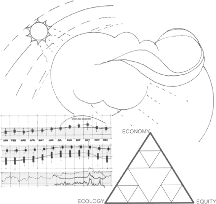
Triple Bottom Line Accounting is a term coined by the British business consultant John Elkington in 1997 that refers to environmental, societal and financial accounting.

This fractal triangle, developed by McDonough and Braungart, is a tool that helps you identify and understand triple bottom line accounting. Each point of the triangle is one of the triple bottom line elements, and points between each illustrate the different combinations of points on each side. Being a fractal, there are infinite combinations possible, just as in human social behavior.[43]
Life Cycle Design (LCD): Where true cost accounting and cradle-to-cradle material cycles become a part of the design process.
More exploration needs to be done to improve the life-cycle sustainability of building materials. Retrofitting existing buildings with local, sustainable materials rather than high-tech, high-environmental cost materials. [96–104]