In this chapter, you will learn the following items:
How to find a data sample's kurtosis and skewness and determine if the sample meets acceptable levels of normality.
How to use SPSS® to find a data sample's kurtosis and skewness and determine if the sample meets acceptable levels of normality.
How to perform a Kolmogorov–Smirnov one-sample test to determine if a data sample meets acceptable levels of normality.
How to use SPSS to perform a Kolmogorov–Smirnov one-sample test to determine if a data sample meets acceptable levels of normality.
2.2 Introduction
Parametric statistical tests, such as the t-test and one-way analysis of variance, are based on particular assumptions or parameters. The data samples meeting those parameters are randomly drawn from a normal population, based on independent observations, measured with an interval or ratio scale, possess an adequate sample size (see Chapter 1), and approximately resemble a normal distribution. Moreover, comparisons of samples or variables should have approximately equal variances. If data samples violate one or more of these assumptions, you should consider using a nonparametric test.
Examining the data gathering method, scale type, and size of a sample are fairly straightforward. However, examining a data sample's resemblance to a normal distribution, or its normality, requires a more involved analysis. Visually inspecting a graphical representation of a sample, such as a stem and leaf plot or a box and whisker plot, might be the most simplistic examination of normality. Statisticians advocate this technique in beginning statistics; however, this measure of normality does not suffice for strict levels of defensible analyses.
In this chapter, we present three quantitative measures of sample normality. First, we discuss the properties of the normal distribution. Then, we describe how to examine a sample's kurtosis and skewness. Next, we describe how to perform and interpret a Kolmogorov–Smirnov one-sample test. In addition, we describe how to perform each of these procedures using SPSS.
2.3 Describing Data and the Normal Distribution
An entire chapter could easily be devoted to the description of data and the normal distribution and many books do so. However, we will attempt to summarize the concept and begin with a practical approach as it applies to data collection.
In research, we often identify some population we wish to study. Then, we strive to collect several independent, random measurements of a particular variable associated with our population. We call this set of measurements a sample. If we used good experimental technique and our sample adequately represents our population, we can study the sample to make inferences about our population. For example, during a routine checkup, your physician draws a sample of your blood instead of all of your blood. This blood sample allows your physician to evaluate all of your blood even though he or she only tested the sample. Therefore, all of your body's blood cells represent the population about which your physician makes an inference using only the sample.
While a blood sample leads to the collection of a very large number of blood cells, other fields of study are limited to small sample sizes. It is not uncommon to collect less than 30 measurements for some studies in the behavioral and social sciences. Moreover, the measurements lie on some scale over which the measurements vary about the mean value. This notion is called variance. For example, a researcher uses some instrument to measure the intelligence of 25 children in a math class. It is highly unlikely that every child will have the same intelligence level. In fact, a good instrument for measuring intelligence should be sensitive enough to measure differences in the levels of the children.
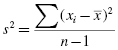
The variance s2 can be expressed quantitatively. It can be calculated using Formula 2.1:
where xi is an individual value in the distribution, is the distribution's mean, and n is the number of values in the distribution
As mentioned in Chapter 1, parametric tests assume that the variances of samples being compared are approximately the same. This idea is called homogeneity of variance. To compare sample variances, Field (2005) suggested that we obtain a variance ratio by taking the largest sample variance and dividing it by the smallest sample variance. The variance ratio should be less than 2. Similarly, Pett (1997) indicated that no sample's variance be twice as large as any other sample's variance. If the homogeneity of variance assumption cannot be met, one would use a nonparametric test.
A more common way of expressing a sample's variability is with its standard deviation, s. Standard deviation is the square root of variance where . In other words, standard deviation is calculated using Formula 2.2:
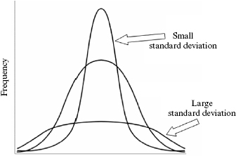
As illustrated in Figure 2.1, a small standard deviation indicates that a sample's values are fairly concentrated about its mean, whereas a large standard deviation indicates that a sample's values are fairly spread out.
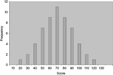
A histogram is a useful tool for graphically illustrating a sample's frequency distribution and variability (see Fig. 2.2). This graph plots the value of the measurements horizontally and the frequency of each particular value vertically. The middle value is called the median and the greatest frequency is called the mode.
The mean and standard deviation of one distribution differ from the next. If we want to compare two or more samples, then we need some type of standard. A standard score is a way we can compare multiple distributions. The standard score that we use is called a z-score, and it can be calculated using Formula 2.3:
where xi is an individual value in the distribution, is the distribution's mean, and s is the distribution's standard deviation.
There is a useful relationship between the standard deviation and z-score. We can think of the standard deviation as a unit of horizontal distance away from the mean on the histogram. One standard deviation from the mean is the same as z = 1.0. Two standard deviations from the mean are the same as z = 2.0. For example, if s = 10 and for a distribution, then z = 1.0 at x = 80 and z = 2.0 at x = 90. What is more, z-scores that lie below the mean have negative values. Using our example, z = −1.0 at x = 60 and z = −2.0 at x = 50. Moreover, z = 0.0 at the mean value, x = 70. These z-scores can be used to compare our distribution with another distribution, even if the mean and standard deviation are different. In other words, we can compare multiple distributions in terms of z-scores.
To this point, we have been focused on distributions with finite numbers of values, n. As more data values are collected for a given distribution, the histogram begins to resemble a bell shape called the normal curve. Figure 2.3 shows the relationship among the raw values, standard deviation, and z-scores of a population. Since we are describing a population, we use sigma, σ, to represent standard deviation and mu, μ, to represent the mean.
The normal curve has three particular properties (see Fig. 2.4). First, the mean, median, and mode are equal. Thus, most of the values lie in the center of the distribution. Second, the curve displays perfect symmetry about the mean. Third, the left and right sides of the curve, called the tails, are asymptotic. This means that they approach the horizontal axis, but never touch it.
When we use a normal curve to represent probabilities p, we refer to it as the normal distribution. We set the area under the curve equal to p = 1.0. Since the distribution is symmetrical about the mean, p = 0.50 on the left side of the mean and p = 0.50 on the right. In addition, the ordinate of the normal curve, y, is the height of the curve at a particular point. The ordinate is tallest at the curve's center and decreases as you move away from the center. Table B.1 in Appendix B provides the z-scores, probabilities, and ordinates for the normal distribution.
2.4 Computing and Testing Kurtosis and Skewness for Sample Normality
A frequency distribution that resembles a normal curve is approximately normal. However, not all frequency distributions have the approximate shape of a normal curve. The values might be densely concentrated in the center or substantially spread out. The shape of the curve may lack symmetry with many values concentrated on one side of the distribution. We use the terms kurtosis and skewness to describe these conditions, respectively.
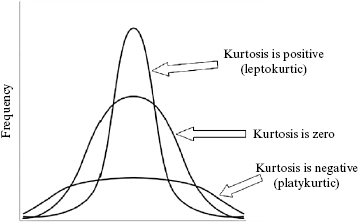
Kurtosis is a measure of a sample or population that identifies how flat or peaked it is with respect to a normal distribution. Stated another way, kurtosis refers to how concentrated the values are in the center of the distribution. As shown in Figure 2.5, a peaked distribution is said to be leptokurtic. A leptokurtic distribution has a positive kurtosis. If a distribution is flat, it is said to be platykurtic. A platykurtic distribution has a negative kurtosis.
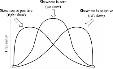
The skewness of a sample can be described as a measure of horizontal symmetry with respect to a normal distribution. As shown in Figure 2.6, if a distribution's scores are concentrated on the right side of the curve, it is said to be left skewed. A left skewed distribution has a negative skewness. If a distribution's scores are concentrated on the left side of the curve, it is said to be right skewed. A right skewed distribution has a positive skewness.
The kurtosis and skewness can be used to determine if a sample approximately resembles a normal distribution. There are five steps for examining sample normality in terms of kurtosis and skewness.
Determine the sample's mean and standard deviation.
Determine the sample's kurtosis and skewness.
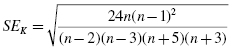
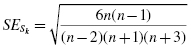
Calculate the standard error of the kurtosis and the standard error of the skewness.
Calculate the z-score for the kurtosis and the z-score for the skewness.
Compare the z-scores with the critical region obtained from the normal distribution.
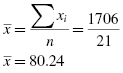
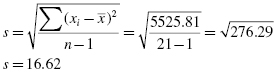
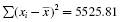
The calculations to find the values for a distribution's kurtosis and skewness require you to first find the sample mean and the sample standard deviation s. Recall that standard deviation is found using Formula 2.2. The mean is found using Formula 2.4:
Normality can be evaluated using the z-score for the kurtosis, zK, and the z-score for the skewness, . Use Formula 2.9 and Formula 2.10 to find those z-scores:
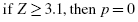
Compare these z-scores with the values of the normal distribution (see Table B.1 in Appendix B) for a desired level of confidence α. For example, if you set α = 0.05, then the calculated z-scores for an approximately normal distribution must fall between −1.96 and +1.96.
2.4.1 Sample Problem for Examining Kurtosis
The scores in Table 2.1 represent students' quiz performance during the first week of class. Use α = 0.05 for your desired level of confidence. Determine if the samples of week 1 quiz scores are approximately normal in terms of its kurtosis.
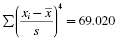
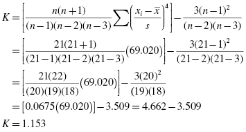
Use the values for the mean and standard deviation to find the kurtosis. Again, it is helpful to set up Table 2.3 to manage the summation when computing the kurtosis (see Formula 2.5).
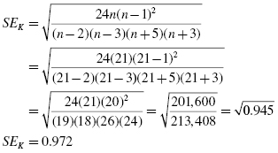
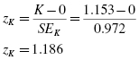
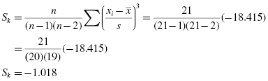
Finally, use the kurtosis and the standard error of the kurtosis to find a z-score:
Use the z-score to examine the sample's approximation to a normal distribution. This value must fall between −1.96 and +1.96 to pass the normality assumption for α = 0.05. Since this z-score value does fall within that range, the sample has passed our normality assumption for kurtosis. Next, the sample's skewness must be checked for normality.
2.4.2 Sample Problem for Examining Skewness
Based on the same values from the example listed earlier, determine if the samples of week 1 quiz scores are approximately normal in terms of its skewness.
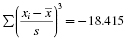
Use the mean and standard deviation from the previous example to find the skewness. Set up Table 2.4 to manage the summation in the skewness formula.
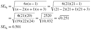
Finally, use the skewness and the standard error of the skewness to find a z-score:
Use the z-score to examine the sample's approximation to a normal distribution. This value must fall between −1.96 and +1.96 to pass the normality assumption for α = 0.05. Since this z-score value does not fall within that range, the sample has failed our normality assumption for skewness. Therefore, either the sample must be modified and rechecked or you must use a nonparametric statistical test.
2.4.3 Examining Skewness and Kurtosis for Normality Using SPSS
We will analyze the examples earlier using SPSS.
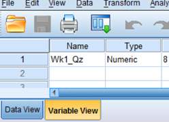
2.4.3.1 Define Your Variables
First, click the “Variable View” tab at the bottom of your screen. Then, type the name of your variable(s) in the “Name” column. As shown in Figure 2.7, we have named our variable “Wk1_Qz.”
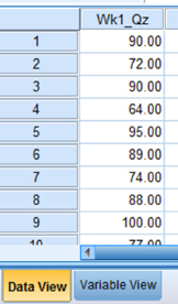
Click the “Data View” tab at the bottom of your screen and type your data under the variable names. As shown in Figure 2.8, we have typed the values for the “Wk1_Qz” sample.
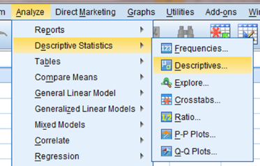
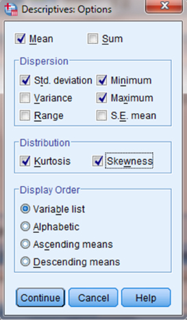
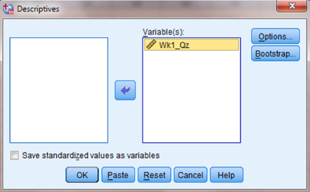
Choose the variable(s) that you want to examine. Then, click the button in the middle to move the variable to the “Variable(s)” box, as shown in Figure 2.10. Next, click the “Options …” button to open the “Descriptives: Options” window shown in Figure 2.11. In the “Distribution” section, check the boxes next to “Kurtosis” and “Skewness.” Then, click “Continue.”
2.4.3.4 Interpret the Results from the SPSS Output Window
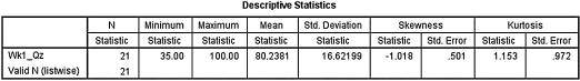
The SPSS Output 2.1 provides the kurtosis and the skewness, along with their associated standard errors. In our example, the skewness is −1.018 and its standard error is 0.501. The kurtosis is 1.153 and its standard error is 0.972.
At this stage, we need to manually compute the z-scores for the skewness and kurtosis as we did in the previous examples. First, compute the z-score for kurtosis:
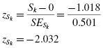
Next, we compute the z-score for skewness:
Both of these values must fall between −1.96 and +1.96 to pass the normality assumption for α = 0.05. The z-score for kurtosis falls within the desired range, but the z-score for skewness does not. Using α = 0.05, the sample has passed the normality assumption for kurtosis, yet failed the normality assumption for skewness. Therefore, either the sample must be modified and rechecked or you must use a nonparametric statistical test.
2.5 Computing the Kolmogorov–Smirnov One-Sample Test
The Kolmogorov–Smirnov one-sample test is a procedure to examine the agreement between two sets of values. For our purposes, the two sets of values compared are an observed frequency distribution based on a randomly collected sample and an empirical frequency distribution based on the sample's population. Furthermore, the observed sample is examined for normality when the empirical frequency distribution is based on a normal distribution.
The Kolmogorov–Smirnov one-sample test compares two cumulative frequency distributions. A cumulative frequency distribution is useful for finding the number of observations above or below a particular value in a data sample. It is calculated by taking a given frequency and adding all the preceding frequencies in the list. In other words, it is like making a running total of the frequencies in a distribution. Creating cumulative frequency distributions of the observed and empirical frequency distributions allow us to find the point at which these two distributions show the largest divergence. Then, the test uses the largest divergence to identify a two-tailed probability estimate p to determine if the samples are statistically similar or different.
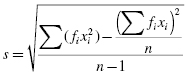
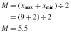
To perform the Kolmogorov–Smirnov one-sample test, we begin by determining the relative empirical frequency distribution based on the observed sample. This relative empirical frequency distribution will approximate a normal distribution since we are examining our observed values for sample normality. First, calculate the observed frequency distribution's midpoint M and standard deviation s. The midpoint and standard deviation are found using Formula 2.11 and Formula 2.12:
where xi is a given value in the observed sample, fi is the frequency of a given value in the observed sample, and n is the number of values in the observed sample.
Next, use the midpoint and standard deviation to calculate the z-scores (see Formula 2.13) for the sample values xi,
Use those z-scores and Table B.1 in Appendix B to determine the probability associated with each sample value, . These p-values are the relative frequencies of the empirical frequency distribution .
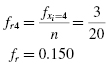
Now, we find the relative values of the observed frequency distribution fr. Use Formula 2.14:
where fi is the frequency of a given value in the observed sample and n is the number of values in the observed sample.
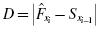
Since the Kolmogorov–Smirnov test uses cumulative frequency distributions, both the relative empirical frequency distribution and relative observed frequency distribution must be converted into cumulative frequency distributions and , respectively. Use Formula 2.15 and Formula 2.16 to find the absolute value divergence and D between the cumulative frequency distributions:
A p-value that exceeds the level of risk associated with the null hypothesis indicates that the observed sample approximates the empirical sample. Since our empirical distributions approximated a normal distribution, we can state that our observed sample is sufficiently normal for parametric statistics. Conversely, a p-value that is smaller than the level of risk indicates an observed sample that is not sufficiently normal for parametric statistics. The nonparametric statistical tests in this book are useful if a sample lacks normality.
2.5.1 Sample Kolmogorov–Smirnov One-Sample Test
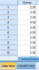
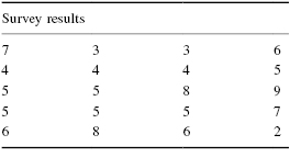
A department store has decided to evaluate customer satisfaction. As part of a pilot study, the store provides customers with a survey to rate employee friendliness. The survey uses a scale of 1–10 and its developer indicates that the scores should conform to a normal distribution. Use the Kolmogorov–Smirnov one-sample test to decide if the sample of customers surveyed responded with scores approximately matching a normal distribution. The survey results are shown in Table 2.5.
The null hypothesis states that the observed sample has an approximately normal distribution. The research hypothesis states that the observed sample does not approximately resemble a normal distribution.
The null hypothesis is
HO: There is no difference between the observed distribution of survey scores and a normally distributed empirical sample.
The research hypothesis is
HA: There is a difference between the observed distribution of survey scores and a normally distributed empirical sample.
2.5.1.2 Set the Level of Risk (or the Level of Significance) Associated with the Null Hypothesis
The level of risk, also called an alpha (α), is frequently set at 0.05. We will use an α = 0.05 in our example. In other words, there is a 95% chance that any observed statistical difference will be real and not due to chance.
2.5.1.3 Choose the Appropriate Test Statistic
We are seeking to compare our observed sample against a normally distributed empirical sample. The Kolmogorov–Smirnov one-sample test will provide this comparison.
2.5.1.4 Compute the Test Statistic
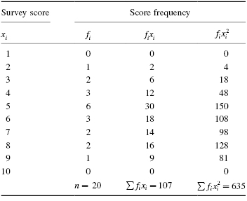
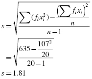
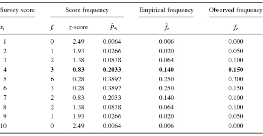
First, determine the midpoint and standard deviation for the observed sample. Table 2.6 helps to manage the summations for this process.
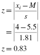
We will provide a sample calculation for survey score = 4 as seen in Table 2.7. Use Formula 2.13 to calculate the z-scores:
Use each z-score and Table B.1 in Appendix B to determine the probability associated with the each value, :
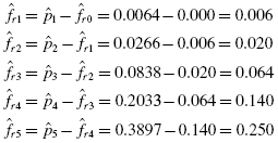
To find the empirical frequency value for each value, subtract its preceding value,, from the associated probability value . In other words,
We establish our empirical frequency distribution beginning at the tail, xi = 1, and work to the midpoint, xi = 5:
Our empirical frequency distribution is based on a normal distribution, which is symmetrical. Therefore, we can complete our empirical frequency distribution by basing the remaining values on a symmetrical distribution. Those values are in Table 2.7.
Now, we find the values of the observed frequency distribution fr with Formula 2.14. We provide a sample calculation with survey result = 4. That survey value occurs three times:
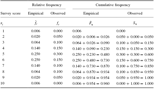
Next, we create cumulative frequency distributions using the empirical and observed frequency distributions. A cumulative frequency distribution is created by taking a frequency and adding all the preceding values. We demonstrate this in Table 2.8.
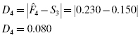
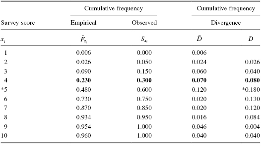
Now, we find the absolute value divergence and D between the cumulative frequency distributions. Use Formula 2.15 and Formula 2.16. See the sample calculation for survey score = 4 as seen in bold in Table 2.9.
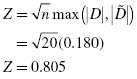
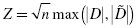
To find the test statistic Z, use the largest value from and D in Formula 2.17. Table 2.9 has an asterisk next to the largest divergence. That value is located at survey value = 5. It is :
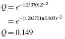
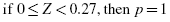
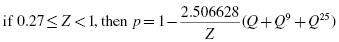
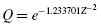
2.5.1.5 Determine the p-Value Associated with the Test Statistic
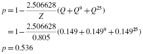
2.5.1.6 Compare the p-Value with the Level of Risk (or the Level of Significance) Associated with the Null Hypothesis
The critical value for rejecting the null hypothesis is α = 0.05 and the obtained p-value is p = 0.536. If the critical value is greater than the obtained value, we must reject the null hypothesis. If the critical value is less than the obtained p-value, we must not reject the null hypothesis. Since the critical value is less than the obtained value (0.05 < 0.536), we do not reject the null hypothesis.
2.5.1.7 Interpret the Results
We did not reject the null hypothesis, suggesting the customers' survey ratings of employee friendliness sufficiently resembled a normal distribution. This means that a parametric statistical procedure may be used with this sample.
2.5.1.8 Reporting the Results
When reporting the results from the Kolmogorov–Smirnov one-sample test, we include the test statistic (D), the degrees of freedom (which equals the sample size), and the p-value in terms of the level of risk α. Based on our analysis, the sample of customers is approximately normal, where D(20) = 0.180, p > 0.05.
2.5.2 Performing the Kolmogorov–Smirnov One-Sample Test Using SPSS
We will analyze the data from the example earlier using SPSS.
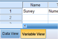
2.5.2.1 Define Your Variables
First, click the “Variable View” tab at the bottom of your screen. Then, type the names of your variables in the “Name” column. As shown in Figure 2.13, the variable is called “Survey.”
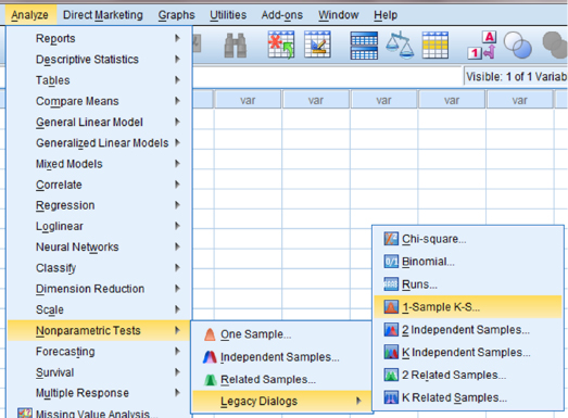
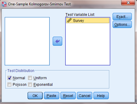
Use the arrow button to place your variable with your data values in the box labeled “Test Variable List:” as shown in Figure 2.16. Finally, click “OK” to perform the analysis.
2.5.2.4 Interpret the Results from the SPSS Output Window
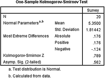
SPSS Output 2.2 provides the most extreme difference (D = 0.176), Kolmogorov–Smirnov Z-test statistic (Z = 0.789), and the significance (p = 0.562). Based on the results from SPSS, the p-value exceeds the level of risk associated with the null hypothesis (α = 0.05). Therefore, we do not reject the null hypothesis. In other words, the sample distribution is sufficiently normal.
On an added note, differences between the values from the sample problem earlier and the SPSS output are likely due to value precision and computational round off errors.
2.6 Summary
Parametric statistical tests, such as the t-test and one-way analysis of variance, are based on particular assumptions or parameters. Therefore, it is important that you examine collected data for its approximation to a normal distribution. Upon doing that, you can consider whether you will use a parametric or nonparametric test for analyzing your data.
In this chapter, we presented three quantitative measures of sample normality. First, we described how to examine a sample's kurtosis and skewness. Then, we described how to perform and interpret a Kolmogorov–Smirnov one-sample test. In the following chapters, we will describe several nonparametric procedures for analyzing data samples that do not meet the assumptions needed for parametric statistical tests. In the chapter that follows, we will begin by describing a test for comparing two unrelated samples.
2.7 Practice Questions
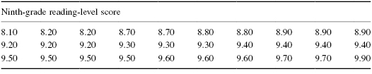
1. The values in Table 2.10 are a sample of reading-level score for a 9th-grade class. They are measured on a ratio scale. Examine the sample's skewness and kurtosis for normality for α = 0.05. Report your findings.
2. Using a Kolmogorov–Smirnov one-sample test, examine the sample of values from Table 2.10. Report your findings.
At α = 0.05, the sample's skewness fails the normality test, while the kurtosis passes the normality test. Based on our standard of α = 0.05, this sample of reading levels for 9th-grade students is not sufficiently normal.
2.SPSS Output 2.3 shows the results from the Kolmogorov–Smirnov one-sample test.
Kolmogorov–Smirnov obtained value = 1.007
Two-Tailed significance = 0.263
According to the Kolmogorov–Smirnov one-sample test with α = 0.05, this sample of reading levels for 9th-grade students is sufficiently normal.
 is the distribution's mean, and n is the number of values in the distribution
 . In other words, standard deviation is calculated using Formula 2.2:
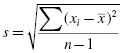

 is the distribution's mean, and s is the distribution's standard deviation.
 for a distribution, then z = 1.0 at x = 80 and z = 2.0 at x = 90. What is more, z-scores that lie below the mean have negative values. Using our example, z = −1.0 at x = 60 and z = −2.0 at x = 50. Moreover, z = 0.0 at the mean value, x = 70. These z-scores can be used to compare our distribution with another distribution, even if the mean and standard deviation are different. In other words, we can compare multiple distributions in terms of z-scores.
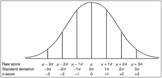

 and the sample standard deviation s. Recall that standard deviation is found using
 is the sum of the values in the sample and n is the number of values in the sample.
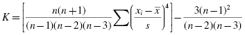
 , are found using
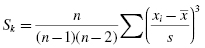
 . Use
. Use 


 based on the observed sample. This relative empirical frequency distribution will approximate a normal distribution since we are examining our observed values for sample normality. First, calculate the observed frequency distribution's midpoint M and standard deviation s. The midpoint and standard deviation are found using
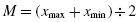

 . These p-values are the relative frequencies of the empirical frequency distribution
  .
.
 and
and  , respectively. Use
  and D between the cumulative frequency distributions:


 :
: 
 for each value, subtract its preceding value,
 , from the associated probability value
  . In other words,
 and D between the cumulative frequency distributions. Use
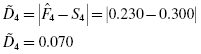
 and D in
  :
: