3

Impact of Competition Policy on Collusion

This chapter reviews theoretical research as it pertains to understanding the impact of competition law and enforcement on collusion. Section 3.1 examines how it affects whether a cartel forms and, if one does form, how long the cartel lasts. Given that a cartel forms, section 3.2 looks into how competition law and enforcement influences which firms participate. Finally, section 3.3 discusses how competition law and enforcement impacts the prices set by colluding firms. The Appendix provides a list of notation for easy reference.

3.1   Cartel Formation and Duration

In investigating how competition policy affects whether there is collusion, it is useful to consider how this question is posed in a game-theoretic framework. Most papers do not model cartel formation but instead ask how competition policy affects the conditions for a collusive equilibrium to exist. From that perspective, cartel formation is said to be less likely when the collusive equilibrium conditions are more stringent. If one imagines industries differing in terms of the model’s parameters, then a more stringent equilibrium condition translates into a smaller set of industries (that is, a smaller set of parameter constellations) for which collusion is stable (in the sense of being supported by an equilibrium). A very good application of this approach is Chen and Rey (2013). An alternative method is to specify a set of industries and explicitly model the birth and death process of cartels. An attractive feature of those models is that it allows the derivation of average cartel duration and the steady-state presence of cartels. Such a modeling perspective is taken in Harrington and Chang (2009, 2015).

3.1.1   Impact of Competition Policy on the Set of Markets for Which Collusion Is Stable

Let us begin by putting forth a simple model to explore how competition law and enforcement impacts the existence of a collusive equilibrium.1 Consider an infinitely repeated game in which the stage game is an n-firm Prisoners’ Dilemma. Let πⁿ denote the noncollusive (static Nash equilibrium) per period profit, so the present value of the noncollusive profit stream is Vⁿ ≡ πⁿ/(1 − δ), where the common discount factor is δ ∈ (0, 1). The per period collusive profit is π^c(>πⁿ), and suppose that firms sustain collusion using the grim punishment; that is, deviation from the collusive outcome results in permanent reversion to the noncollusive outcome. As long as firms collude, a firm will have a constant profit stream of π^c, which has a present value of π^c/(1 − δ). If a firm deviates from the collusive outcome, it earns profit π^d(>π^c) in that period and, as a consequence of the grim punishment, πⁿ thereafter. Thus, in the absence of competition law, collusion is sustainable (that is, the grim trigger strategy is a subgame perfect equilibrium) if and only if

In each period that firms are colluding, there is an exogenous probability σ ∈ (0, 1) that the cartel is discovered, prosecuted, and convicted. In that event, firms are levied a penalty and are assumed not to collude thereafter.² The penalty scheme has each firm assessed an amount f > 0 for each period the cartel was in place. In principle, if the cartel colluded for T periods prior to conviction then they are liable for a penalty of f T. In practice, the penalty is generally less than that value, because it is based on documented cartel duration rather than true cartel duration. So as to capture the deterioration of evidence, penalties are assumed to decay. If F^t is the penalty that a firm would have to pay if caught and convicted in period t, it is assumed to evolve as follows: F^t = βF^t−1 + f, where 1 − β ∈ (0, 1) is the depreciation rate. For technical reasons, it is important for the penalty to depreciate so that it is bounded.

Assuming that, on the equilibrium path, collusion is sustainable in all periods, V^c(F) denotes the collusive value given an accumulated penalty of F. It is defined recursively by

and can be shown to equal

The first term is the expected present value of profits from the product market, and the second term is the expected discounted penalty.

Assuming the cartel starts operating in period 1, then F⁰ = 0 and, on the equilibrium path, F^t ∈ [0, f /(1 − β)], ∀t ≥ 1, where f /(1 − β) is the steady-state penalty. Equilibrium requires that the payoff from colluding, V^c(F), is at least as great as the payoff from deviating. In specifying the deviation payoff, it is assumed that the cartel could be caught in the current period but has no chance of being caught in the future. The equilibrium conditions are then

One can show that this equilibrium condition is more stringent when F is higher. Intuitively, given that firms are more likely to end up paying penalties when they continue colluding, deviation (with subsequent cartel breakdown) becomes more attractive as the accumulated penalty grows. As a result, (3.3) holds if and only if it holds for the steady-state penalty of f /(1 − β). Setting F equal to f /(1 − β) in (3.2), we can solve for the steady-state collusive value:

Inserting this expression into (3.3) yields the necessary and sufficient condition for collusion to be stable:

Collusion is said to be deterred if and only if (3.4) does not hold. Of course, if (3.4) holds, then collusion can occur but need not occur; just because an equilibrium with collusion exists does not mean that collusion will occur: there is always an equilibrium without collusion. It is worth noting that collusion can be more profitable than competition—V^c( f /(1 − β)) > Vⁿ—yet (3.4) is not satisfied. As noted by Buccirossi and Spagnolo (2007), deterrence of cartel formation only requires that competition policy make collusion unstable, not unprofitable.

If we consider the Bertrand price game, then πⁿ = 0 and π^d = nπ^c, in which case (3.4) can be simplified and rearranged to

Suppose industries are identical except for the price of the next best substitute, and that results in variation in the collusive profit π^c. Expression (3.5) says that collusion is possible only in those industries for which π^c ≥ Ψ(σ, f, β). The Ψ(σ, f, β) is larger when competition policy is tougher—as reflected in a higher probability of being caught and convicted σ, a higher penalty f, and more effective documentation of evidence as reflected in a higher β—so more industries are immune to collusion.³ While both the collusive payoff (on the left-hand side, LHS) and the deviation payoff (on the right-hand side, RHS) in (3.4) are increasing in σ, f, and β, it is straightforward to show that the LHS is more sensitive to the policy parameters—because penalties are more likely to be incurred when firms continue colluding—in which case the equilibrium condition is more stringent.

3.1.2   Impact of Competition Policy on the Cartel Rate

An alternative approach to exploring how competition policy impacts the prevalence of collusion is to explicitly model the birth and death process of cartels. While there is some research that endogenizes cartel formation,4 the only work that models the birth and death process of cartels is Harrington and Chang (2009, 2015).

Modifying the infinitely repeated n-firm Prisoners’ Dilemma, suppose market demand is stochastically realized which produces a potential profit that a firm can earn that is denoted by π. The variable π is independently drawn each period according to the differentiable cdf , and denotes its finite mean. Collusive profit is equal to that potential profit: π^c = π. As in Rotemberg and Saloner (1986), π is observed prior to firms deciding how to behave. The profit from deviating is π^d = ηπ, where η > 1, and the noncollusive profit is πⁿ = απ, where α ∈ [0, 1).

At any point in time, an industry is either cartelized or not, and moves in and out of the cartel state as follows. Suppose it is currently a cartel. In response to the realization of the profit state π, collusion may not be incentive compatible (i.e., it is not an equilibrium). In that case, the cartel collapses, each firm earns απ, and the industry shifts to the non-cartel state. If collusion is incentive compatible, then each firms earn π. Whether the cartel collapsed or remained intact, there is a probability σ that the cartel is caught and convicted. If it is convicted, then the industry shifts to the non-cartel state. If instead the industry is not a cartel, then it has a probability κ ∈ (0, 1) of moving to the cartel state.

In modeling a population of industries, the industries are allowed to vary in terms of cartel stability as captured by the parameter η, which controls the amount of profit gained by cheating. The differentiable cdf on industry types is , where .

Let V^c denote the firm value in the cartel state and V^nc denote the firm value in the non-cartel state. In the event that a cartel is convicted, the penalty levied on a firm is γ ([1 − δ]V^c − αμ), where γ > 0 and αμ is average noncollusive profit. This specification allows the penalty to be sensitive to the average incremental gain from colluding. The equilibrium condition is

Noting that the non-cartel value is defined by V^nc = (1 − κ)(αμ + δV^nc) + κV^c, one can use it in (3.6) to show that the equilibrium condition holds if and only if

Just as in Rotemberg and Saloner (1986), collusion is stable when the profit realization is sufficiently low. When profit is high, the increase in current profit from deviating is large, while the continuation payoff is unaffected (as π is iid over time).

The next step is to solve for the equilibrium value for V^c. Given that an industry is cartelized and given that π ≤ ϕ(V^c, η), each firm earns collusive profits π. The cartel is caught with probability σ, in which case each firm receives the future payoff V^nc less the penalty, and if not caught, then each earns the future collusive value V^c. If instead π > ϕ(V^c, η), then the cartel collapses, so each firm earns απ and the future value is V^nc less expected penalties. The following equation then defines the implied collusive value, ψ(V^c), when firms perceive it to be V^c:

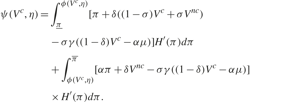
A fixed point of ψ is an equilibrium value for V^c. One fixed point is the noncollusive value, V^c = αμ/(1 − δ). If σ and γ are sufficiently low, then there is also at least one solution in which firms collude, V^c > αμ/(1 − δ). When there are multiple solutions, it is assumed that the maximal solution is selected, and it is denoted by V^c*(η). The value attached to being in the cartel state, V^c*(η), is lower when the likelihood of conviction σ is higher, the penalty multiple γ is higher, and the cartel is inherently less stable (i.e., a higher value for η).

Given V^c*(η), define ϕ^*(η) as the maximum profit realization such that the cartel is stable: ϕ^*(η) ≡ ϕ(V^c*(η), η) using (3.7). The variable ϕ^*(η) is a measure of cartel stability, since the cartel is stable if and only if π ≤ ϕ^*(η). This can be seen more clearly by noting that the probability a cartel survives in any period is (1 − σ)H(ϕ^*(η)), which is the probability of the joint event that it is not caught, 1 − σ, and that it does not internally collapse, H(ϕ^*(η)). It can be shown that (1 − σ)H(ϕ^*(η)) is increasing in η, so that cartels whose firms have a higher temptation to deviate (higher η) collapse for lower profit states (ϕ^*(η) is lower) and thus have shorter duration.

At this stage, we can assess the impact of competition policy on the average duration of a cartel. A higher value for σ mechanically means a higher chance that a cartel is shut down because it is caught and convicted. But a higher value for σ (as well as a higher value for γ) also has an indirect effect on cartel duration. A tougher competition policy lowers the cartel value V^c*(η), which then makes the cartel less stable, as reflected in a lower profit threshold ϕ^*(η) at which the cartel collapses, for ϕ^*(η) is decreasing in σ and γ. Thus, even when a CA does not directly shut down a cartel, it indirectly does so by making internal collapse more likely.

What has been described is a Markov birth and death process for each cartel, from which we can derive a steady-state frequency of cartels. For a continuum of industries of type η, let C(η) denote the proportion of cartels among type-η industries. The stationary proportion of type-η industries that are not cartels is defined by

Of the 1 −C(η) industries in the previous period that did not have cartels, a fraction (1 − κ) of them are still not cartels (because they did not have the opportunity to cartelize). In addition, a fraction κ(1 − H(ϕ^*(η))) are not cartels because, while they had the opportunity to cartelize, it was not incentive compatible. And finally, a fraction κH(ϕ^*(η))σ are not cartels because, while they had the opportunity to cartelize and it was incentive compatible to do so, they were caught and convicted. Of the C(η) industries in the previous period that did have cartels, a fraction (1 − H(ϕ^*(η))) internally collapsed, and a fraction H(ϕ^*(η))σ did not collapse but were convicted. Solving (3.8) for C(η) and aggregating across all industry types, the cartel rate (that is, the fraction of all industries cartelized according to the stationary distribution) is

If the penalty rate γ is not too high, then C > 0 and C is decreasing in σ.

The attractiveness of this approach is that it explicitly models the birth and death of cartels and thereby is able to assess the impact of competition policy on cartel duration and the frequency of cartels. A harsher competition policy reduces the cartel rate by deterring cartel formation in some industries (that is, expanding the set of industry types for which collusion is never an equilibrium) and reducing cartel duration in other industries (by lowering ϕ^*(η) and thereby reducing the frequency with which the industry is in the cartel state).

Another deliverable of Harrington and Chang (2009) is providing a way in which to test policy efficacy. It is shown that a rise in the probability of detection and conviction σ causes the immediate collapse of the least stable cartels (that is, those with the highest values of η). This means the surviving cartels are those with lower values of η and thus longer duration. Since this is the pool from which one draws discovered cartels, the average duration of discovered cartels rises in the short run in response to a higher value for σ. Inverting this result, consider a policy that is intended to alter the likelihood of detection and conviction, but the question is whether it succeeded (σ rose), is ineffective (σ is unchanged), or is counterproductive (σ fell). What actually happened can be inferred by observing the duration of discovered cartels in the short run. If average cartel duration goes up (down) then the policy has caused σ to rise (fall) and thus it can be concluded that it will result in fewer (more) cartels forming in the new steady state. Intuitively, if the new policy is effective, then its adoption will immediately cause the marginally stable cartels to collapse, which, by virtue of being marginally stable, tend to be of relatively short duration. Their exit from the cartel population means they cannot be discovered. It follows that the surviving cartels are those which tend to be more stable and thus of longer duration. Since those cartels make up the pool from which cartels are discovered, the average duration of discovered cartels rises in the short run in response to a more effective competition policy.

There are at least two problematic aspects to the approach of Harrington and Chang (2009, 2015). First, the modeling of the birth process is largely devoid of economic content. The opportunity to cartelize is exogenous and unrelated to any incentives to form a cartel.⁵ Second, cartel collapse occurs in the context of the Prisoners’ Dilemma only because firms cannot adjust the extent to which they collude; thus, collusion is either stable or not. If the stage game was a quantity game or differentiated products price game with an infinite action space, then in response to strong demand conditions and a heightened desire to cheat, firms could reduce the extent of collusion rather than end collusion altogether. As cartel collapse is a real phenomenon, the modeling challenge is to generate a positive probability of collapse when the action space is rich.⁶

It is worth noting that Katsoulacos, Motchenkova, and Ulph (2015a) is related on some dimensions to Harrington and Chang (2009, 2015). It similarly considers a population of industries for which cartels are born and die. However, as it does not allow for stochastic market conditions, it cannot produce internal cartel collapse as an equilibrium phenomenon. However, it is richer in allowing for the probability that a cartel reforms to depend on how the cartel died; whether it died because it was caught and convicted or because a member firm cheated (with only the former occurring in equilibrium). The model also introduces another competition policy instrument: the probability that a conviction results in the cartel actually shutting down (rather than the standard assumption that it discontinues for sure). The paper distinguishes between competition policy designed to deter short-term recidivism (which pertains to the probability that a cartel continues post-conviction) and to deter long-term recidivism (which pertains to the probability that a competitive industry cartelizes). The paper provides a rich and promising framework for assessing the welfare impact of competition policy.

3.2   Cartel Participation

Though many cartels are not all-inclusive,7 very little research has been done that examines which firms choose to participate in cartels (and how cartel and non-cartel members interact) and even less work that looks into the influence of competition policy on cartel size and participation. Here we review an approach taken in Bos and Harrington (2010, 2015).⁸

Consider an infinitely repeated capacity-constrained Bertrand price game with perfect monitoring. Firms are identical except possibly with respect to their capacities; n firms offer homogeneous products with identical constant marginal cost c. The capacity of firm j is denoted by k_j and is fixed; is industry capacity, and is total capacity of cartel Γ ⊆ {1, 2, . . . , n}. With market demand D(p), D(p) − (K − K_Γ) is the cartel’s residual demand.

The focus is on equilibrium strategy profiles for which (1) past behavior by non-cartel members has no effect on cartel members’ current behavior, (2) any deviation from the collusive price by a cartel member results in infinite reversion to a static Nash equilibrium, and (3) cartel members set a common price and allocate demand proportional to capacity. Of particular note, (1) means that cartel members do not engage in exclusionary activities against non-cartel members for selling too much. As a result, each non-cartel member’s pricing behavior is its static best response, which is to undercut the collusive price and produce up to capacity. Encompassing exclusionary activities is a worthwhile research direction.

Cartel Γ faces the problem of choosing a common price to maximize each cartel member’s profit while ensuring that the equilibrium condition is satisfied:

As the objective in (3.9) is proportional to a firm’s capacity, all cartel members have the same preferences regarding price; and the equilibrium condition in (3.10) is the same for all firms.

The equilibrium collusive value for firm i ∈ Γ is

In equilibrium, members of cartel Γ price at p^*(Γ) and proportionally constrain output below capacity, while non-cartel members price just below p^*(Γ) and produce at capacity. It is shown that if the cartel controls more capacity, then the cartel price is (weakly) higher: if K_Γ^′′ > K_Γ^′, then p^*(Γ^′′) ≥ p^*(Γ^′).

The focus is on stable cartels in the sense of membership or participation. A cartel is stable if (1) all cartel members prefer to be in the cartel (internal stability), and (2) all non-cartel members prefer to be outside the cartel (external stability). In characterizing the set of stable cartels, first note that cartel members always want non-cartel members to join. It is better to have a firm inside the cartel (restricting its output below its capacity) than outside the cartel (producing at capacity). Formally, if the cartel is more inclusive, then the original cartel members are better off:

In contrast, a non-cartel member may or may not want to join. Joining a cartel has the benefit that it results in a higher collusive price, because the cartel controls more capacity. However, the firm must reduce its supply, as now it is expected to produce below its capacity.

Some insight can be provided as to who is likely to be a member of a stable cartel. First, a firm with more capacity is more inclined to join the cartel, because the rise in price from joining is large relative to the proportional fall in its quantity. Second, if a firm is sufficiently small, it will not join the cartel, because the rise in price is small—as cartel capacity expands only a little—but the percentage by which it must reduce its supply is not small.

Bos and Harrington (2015) augment this structure by introducing competition law and enforcement. There is a per period probability σ(Γ) that cartel Γ ends up paying a penalty. It is assumed that a cartel with more members is more likely to be discovered and convicted: if Γ^′ ⊂ Γ^′′, then σ(Γ^′) < σ(Γ^′′). The penalty to firm i in the event of conviction equals γk_iV^c(Γ) and thus is assumed to be proportional to collusive value. In sum, the expected penalty of firm i ∈ Γ is σ(Γ)γk_iV^c(Γ).

Competition law and enforcement is shown to undermine internal stability and can decrease the size of the largest stable cartel. By joining the cartel, a firm adds to collusive value by having the cartel control more capacity, which results in a higher collusive price. However, more members make it more likely the cartel will be caught and convicted, which raises expected penalties. Thus, the value of being in a cartel can rise when one of its members leave (especially so when the exiting firm is small). Hence, it is no longer the case that a cartel welcomes all firms. This force tends to reduce the size of the largest stable cartel. At the same time, enforcement can increase the size of the smallest stable cartel by undermining internal stability. The expected penalty reduces the collusive value, which tightens the equilibrium condition and so could cause a partial cartel to lose the ability to sustain a collusive price. Ensuring compliance with the collusive price may require making the cartel more inclusive. In sum, it appears that competition policy tends to compress cartel size, in that it makes the smallest stable cartels more inclusive and the largest stable cartels less inclusive.

3.3   Collusive Price

How does competition law and enforcement affect collusive outcomes? In practice, the collusive outcome generally means a common price and a market allocation. However, the literature has almost exclusively focused on the case of symmetric firms, so the only issue is price (with firms having equal market shares).

In thinking about the impact of competition policy on price, it is useful to consider it in the context of a broader question: What constrains the collusive price path? A cartel may not set a higher price, because a higher price is unstable; that is, the equilibrium condition is binding at the current price. Related to that factor, firms may be uncertain about how high a price is stable (e.g., there may be uncertainty regarding firms’ demand functions at a higher price).9 Alternatively, a higher price may be stable but unprofitable. Some possible reasons that it would be unprofitable are that the current price is the monopoly price (so that collusion is maximal), (industrial) buyers may resist a higher price (by postponing their purchases), and a higher price (or a bigger price change) may be more likely to lead to discovery of the cartel.

In the ensuing analysis, the focus is on how competition policy influences price when price affects the likelihood of detection (and conviction) and the magnitude of the penalty in the event of conviction. One modeling approach is to modify a static joint profit maximization model by allowing for conviction and penalties (Block, Nold, and Sidak 1981). Let π(p) denote the representative firm’s profit when all firms charge a common price p, σ(p) the probability of discovery and conviction, and F(p) the per firm penalty if convicted. Assume σ(p) and F(p) are both differentiable and increasing in price, so that a higher price makes discovery more likely and results in a higher penalty (as would be the case with customer damages and some government penalty formulas).

The cartel chooses price to maximize profit minus the expected penalty:

Define p^m as the cartel’s price in the absence of competition policy, which, under the usual concavity assumptions, is defined by π^′(p^m) = 0. If σ^′(p^m) > 0 and F^′(p^m) ≥ 0, then the first-order condition implies that competition policy induces the cartel to set a lower price:

By marginally lowering the cartel price below p^m, there is no first-order effect on profit, because π^′(p^m) = 0, but there is a first-order reduction in the expected penalty, because σ^′(p^m)F(p^m) − σ(p^m)F^′(p^m) > 0.

Much of the literature instead uses a dynamic approach to characterize collusive prices in the presence of competition law and enforcement. One class of dynamic models augments a standard infinitely repeated oligopoly game by assuming that there is some probability of conviction and some penalty, both of which are either fixed or depend only on the current price. Section 3.3.1 discusses models for which the probability of paying penalties and the penalty are fixed. A second class of models has the probability of paying penalties and the penalty size depend on current and past prices. By allowing for dependence on past prices, the game is no longer repeated as there are state variables. That approach is reviewed in sections 3.3.2 and 3.3.3.

3.3.1   Infinitely Repeated Game

Consider an oligopoly game with n firms offering symmetrically differentiated products and assume that a firm’s demand is continuously differentiable with regard to all firms’ prices. Let π_i(p₁, . . . , p_n) be the profit function for firm i with the usual properties of quasi-concavity in own price and increasing in other firms’ prices. If firms collude, then there is a per period probability of discovery and conviction σ, which brings with it a fixed per firm penalty F. In the event of conviction, suppose the cartel is permanently shut down with probability ζ and continues with probability 1 − ζ. However, if a firm deviates then the cartel permanently breaks down, so that a stage game Nash equilibrium ensues.10

In specifying the equilibrium condition, let π^d(p) denote a firm’s maximal profit (with respect to its own price) when all other firms price at p. The equilibrium condition for collusive price p is

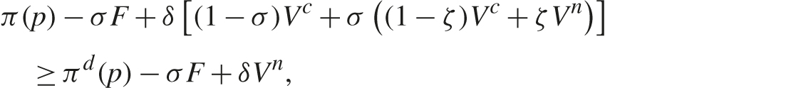
or

where

is the collusive value, and Vⁿ ≡ πⁿ/(1 − δ) is the noncollusive value. Suppose the cartel chooses the price that maximizes the collusive value (3.12) subject to the equilibrium condition (3.11). Given that the expected penalty is independent of price, the optimal collusive price maximizes collusive profit π(p) subject to (3.11). If the equilibrium condition binds, then the optimal collusive price is the highest price such that (3.11) holds.

When competition policy is made more aggressive—as reflected in higher σ and/or higher F—the equilibrium condition (3.11) tightens. If σ and/or F are increased, then the RHS of (3.11) is unaffected, while the LHS is reduced:

A higher penalty F reduces the collusive value, which reduces the payoff from setting the collusive price rather than cheating. A higher probability of paying penalties σ similarly reduces the collusive value but also increases the chances of transiting to the state in which firms are competing. If (3.11) was originally binding, then it no longer holds at the higher values for the policy parameters. If π^d(p) − π(p) (which is the gain in current profit from cheating) is decreasing in the collusive price (which is true under standard assumptions), then the collusive price must be reduced to resatisfy (3.11). Hence, raising the probability of paying penalties or raising the penalty forces the cartel to set a lower price to maintain the internal stability of the collusive arrangement.

In comparing the case of legal cartels (effectively, σ = 0) and illegal cartels (σ > 0), the preceding analysis shows that, given that a cartel forms, prices and therefore markups (how much price is above cost) are lower when cartels are illegal. While that then suggests that collusive markups are lower in jurisdictions for which cartels are illegal, it may also be the case that a prospective cartel that anticipates only being able to support a low markup may find it unprofitable to form, because the incremental profit may be more than offset by the expected penalties. This suggests that we should not see illegal cartels with low markups.

The previous point is made in Bos et al. (2016). To prove it, let us use the preceding model and, for purposes of parsimony, assume ζ = 1, so that conviction shuts down a cartel forever. If cartels are legal (so there is no competition law), the equilibrium condition is

Define pⁿ ∈ arg max π^d(pⁿ) as a symmetric Nash equilibrium price. It can be shown that, for any δ ∈ (0, 1), (3.13) holds as the collusive price gets arbitrarily close to the noncollusive price, p^c → pⁿ. Thus, a legal cartel could, in principle, have very low markups.¹¹ Now consider this setting for illegal cartels. The equilibrium condition is

where

It is easy to show that the equilibrium condition does not hold as p^c → p^N. Given that

it is less profitable to collude than to compete, which implies it is not stable to collude. Hence, a legal cartel could exist with low markups (but still exceed the competitive markup), but an illegal cartel cannot exist with low markups.¹² We already showed above that if a legal cartel has the maximal markup consistent with the equilibrium condition (and it is binding), then the equilibrium condition will be violated with an illegal cartel, which implies that the maximal markup is lower. Hence, markups are higher for legal cartels than for illegal cartels. In sum, competition policy is predicted to compress the distribution of collusive markups, as it reduces the frequency of low markups and high markups.¹³ That prediction is supported by some empirical evidence in Bos et al. (2016).

Thus far it has been shown that competition law and enforcement has the desired impact of making collusion less likely or less extensive. It is possible, however, for it to actually make collusion easier. The preceding analysis was based on competition policy lowering the collusive payoff more than it lowered the deviation payoff, thereby tightening the equilibrium condition and requiring a reduction in the collusive price. Cyrenne (1999) shows that competition policy can lower the punishment payoff sufficiently so that the deviation payoff declines more than the collusive payoff, in which case the equilibrium condition is loosened, thereby allowing for a higher collusive price. That is, in the presence of competition law and enforcement, the payoff to cheating is sufficiently reduced so as to make collusion more stable.

In showing this finding, Cyrenne (1999) modified the imperfect monitoring setting of Porter (1983) and Green and Porter (1984). However, the intuition can be more easily conveyed in the context of a perfect monitoring setting. Let us enrich the preceding model by assuming that the probability of being discovered and convicted varies between (1) when all firms charge the collusive price (denote the probability by σ^co) and (2) when a firm undercuts the collusive price which causes firms to return to competitive pricing (with probability denoted by σ^dev). The equilibrium condition is now

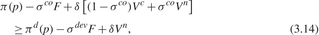
where

Higher σ^co lowers the LHS of (3.14) by lowering V^c and increasing the expected penalty σ^coF. Higher σ^dev lowers the RHS of (3.14) by increasing the expected penalty σ^devF.

Suppose detection is more likely in the event of a deviation: σ^dev > σ^co. If σ^dev is sufficiently higher than σ^co, then the RHS can fall more than the LHS (relative to when there is no competition law and enforcement, so σ^dev = 0 = σ^co) and the equilibrium condition is then loosened. If we fix σ^dev > 0 and let σ^co → 0, then the equilibrium condition becomes

where the LHS is the same as for no competition law, and the RHS is lower. Thus, collusion is easier with competition law and enforcement and, as a result, the illegal cartel can sustain a higher price than the legal cartel can.

This result may be problematic in that the assumption σ^dev > σ^co is motivated by the ensuing price war from a deviation being more likely to trigger detection than a high stable collusive price. While that is quite plausible (and we will later explicitly explore how price changes impact the likelihood of detection), the model ignores the fact that the cartel had to raise price from the competitive level to get to that high stable collusive price, which would also seem to heighten detection and thereby lower the collusive payoff. This criticism aside, Cyrenne (1999) is useful for being one of the first to discuss how detection is impacted by price changes (which is more plausible than it being impacted by price levels) and noting that this could impact equilibrium conditions and thereby the collusive price.

In a related vein, McCutcheon (1997) finds that harsher punishments can be more credible with competition laws. The problem with threatening to impose a really severe punishment (such as not colluding forever or pricing below cost for an extended length of time) is that cartel members would want to renegotiate in the event of a deviation to avoid this self-inflicted harm. The prospect of renegotiation constrains the set of credible punishments and thereby limits how high a collusive price can be sustained. McCutcheon (1997) shows that if competition policy makes meetings among cartel members more costly (by raising the likelihood of discovery), then this could discourage firms from renegotiating a harsh punishment and thereby make those punishments credible. However, just as with the critique of Cyrenne (1999), the impact of competition policy on the initial meetings to form a cartel are ignored, which, in practice, are critical. On the plus side, the analysis highlights the need to formally model meetings and take into account how they are constrained by competition policy.¹⁴

3.3.2   Dynamic Game with State Variables: Exogenous Detection Technology

The models of collusive pricing reviewed thus far have encompassed competition law and enforcement in a rather restrictive manner by assuming that expected penalties are either fixed or depend at most on the collusive price charged in the period in which a cartel is discovered. In reality, the penalty levied on a cartel is cumulative, as it depends on duration and possibly on past overcharges. That feature of actual practice will affect equilibrium conditions. As the cartel is active for a longer span of time, the penalty if caught and convicted rises, which will influence cartel stability. A second feature of reality that has been ignored in these models is that discovery may not just depend on the current price but rather on the price history. For example, buyers may become suspicious if there has been a series of price increases. In this section, research is reviewed that allows the expected penalty—both the probability of conviction and the size of the penalty—to depend on the cartel’s history. This concession to reality introduces a technical complication, because the game is no longer repeated.15

Consider the infinite horizon differentiated products price game described in the preceding section.¹⁶ If the cartel is detected in period t, then each firm pays a penalty X^t and receives noncollusive profit πⁿ thereafter. The penalty X^t evolves over time according to X^t = βX^t−1 + γx(p^t), where x(p^t) > 0 and is nondecreasing, γ > 0, and 1 − β ∈ (0, 1) is the depreciation rate. If the penalty is customer damages, then x(p^t) = (p^t − p^bf)D(p^t), where D(p) is a firm’s demand when all colluding firms charge p, and p^bf is the but-for price (typically, a static Nash equilibrium price). Alternatively, x(p^t) could equal some constant, in which case the penalty just depends on duration. When the cartel comes to set price in period t, it will know the state variable X^t−1, which is the accumulated penalty for each firm.

In allowing past prices to influence the probability of detection, it is assumed only prices in the current period and previous one matter. Let denote the probability of discovery (and conviction) in period t, where is the vector of firms’ prices in period t, and is the price vector for period t − 1. Presuming buyers expect a stable environment, assume that they are more likely to become suspicious when prices change:

and when price increases are larger:

These assumptions are rather mild. However, for some of the ensuing results, a stronger assumption is required, which is that there is a continuously differentiable function and a summary statistic g for a price vector such that

That is, the probability of detection depends on the change in the summary statistic. The following general properties are assumed. First, if all firms charge the same price, then the summary statistic is that price: g(p, . . . , p) = p. Second, a higher price vector increases the summary statistic: if (component wise), then . Average price, weighted average price, and median price all satisfy these properties. Third and finally, it is assumed that is nondecreasing in the summary statistic for price increases—if x ≥ y, then (x) ≥ (y)—and is minimized when the summary statistic does not change, (x) ≥ (0), ∀x. A special case is when the probability of detection is minimized when average price (across firms) does not change and is higher for bigger increases in average price. With these assumptions, detection depends only on price changes and not on the price level.

Along the equilibrium path, the state variables are the accumulated penalty X^t−1 and the cartel’s price in the previous period p^t−1.¹⁷ The setting is one of perfect monitoring, for which if any firm deviates from the collusive price path, then the continuation equilibrium is a Markov perfect equilibrium (hereafter MPE). Given the dynamics associated with detection, even if a firm cheats, the resulting pricing problem is dynamic because the ensuing price path affects the likelihood of detection. While details are in Harrington (2004a), for my purposes here, just let V^mpe denote a firm’s MPE payoff.

The cartel’s problem can be cast as the following constrained dynamic programming problem where, subject to using an MPE punishment, firms achieve the best symmetric subgame perfect equilibrium in terms of expected payoff. Letting V^c(p^t−1, X^t−1) denote a firm’s (equilibrium) value function when firms are colluding, it is recursively defined by

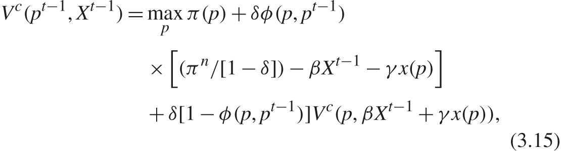
The cartel chooses price while taking into account its impact on current profit π(p), on the probability of detection and conviction ϕ(p, p^t−1), on the penalty βX^t−1 + γx(p), and on the future value V^c(p, βX^t−1 + γx(p)) through its effect on the state variables. It does so while recognizing that the price must be incentive compatible, which requires that the payoff from setting the collusive price is at least as great as that from deviating, as specified in (3.16). In specifying the deviation payoff in (3.16), firm i takes into account its impact on current profit π(p|p_i) (where p|p_i denotes the vector in which all firms but i charge p and firm i charges p_i) and on the probability of being caught and convicted, ϕ(p|p_i, p^t−1). The latter event results in a payoff of (πⁿ/[1 − δ]) − βX^t−1 and, to maintain a common penalty state variable, there is no penalty for the period in which a deviation occurs. In the event that detection does not immediately occur, the continuation payoff is V^mpe(p|p_i, βX^t−1), which is the MPE payoff associated with those state variables.

The comparative advantage of this model is in generating predictions for the entire collusive price path and not just the steady state, which, in essence, is what standard theories provide. Nevertheless, let us start by characterizing the steady-state collusive price (in the event that the cartel has not been caught) when the equilibrium constraint (3.16) is not binding. Letting p^* denote the steady-state price, it is defined by

In the steady state, the price change over time is zero, so the probability of detection is (0). Consider the effect of a one-time marginal change in price from p^*. First, there is the marginal change in current profit of π^′(p^*). Second, there is the marginal change in the accumulated penalty of x^′(P^*), which produces an expected present value loss equal to [δ(0)/(1 − δβ[1 − (0)])]γx^′(p^*) (which takes into account the likelihood of detection as well as penalty depreciation). Third, there is the change in the expected penalty associated with previously incurred penalties, which is ^′(0)[γx(P^*)/(1 −β)], but this equals zero, since ^′(0) = 0 (as is minimized at zero and is differentiable).

As described in (3.17), the steady-state cartel price is set so as to equate the rise in profit from a higher price with the expected present value of the marginal rise in the penalty from that higher price. Note that if the penalty is insensitive to price, x^′(p) = 0, then the second term is zero, so π^′(p^*) = 0, which means that the cartel charges the unconstrained joint profit-maximizing price in the long run. For example, if the penalty only depends on duration—which is captured here with x(p) = f for some f > 0—then competition policy may constrain collusive price in the short run (which we will see below is indeed the case), but it does not constrain collusive price in the long run. What drives this result is that the probability of detection is not sensitive to small price changes, so in the steady-state, there is no first-order effect on the expected penalty from raising price a little. Hence, the cartel will raise price as long as it is below the joint profit-maximizing price. However, it is likely to raise price only gradually, because bigger price changes result in higher chances of detection. Competition policy then slows the rate at which the collusive price converges to the monopoly price.

Let us now turn to examining price dynamics. If the equilibrium conditions in (3.16) are not binding, then it can be shown that the equilibrium price path is increasing over time. This is so for obvious reasons. The probability of detection is increasing in the price change so the cartel gradually raises price to the steady-state level and, in doing so, trades off a lower current profit for a lower chance of detection. Though a straightforward implication of the model’s assumptions, it is still useful to have a theory that produces a transitional price path, because many actual cartels have such price dynamics. As the cartel continues to collude and to do so at higher prices, the accumulated penalty X^t grows, which makes the cartel more sensitive to not inducing detection. As the probability of triggering detection would be higher if price is lowered (compared to keeping price constant), this dynamic provides a reinforcing reason for price not to decline at any point on the collusive price path. That property, however, necessarily holds only when the equilibrium conditions are not binding. If they are binding, then as the penalty accumulates, they can become more stringent. The reason is that the likelihood of paying penalties is lessened by shutting the cartel down, and that enhances the incentive to deviate. In that case, the previous period’s price may no longer be sustainable with a higher accumulated penalty, which forces the cartel to lower price in order to maintain cartel stability. This is true even though lowering price implies a higher chance of detection than does keeping price fixed. Thus, an illegal cartel’s price path could initially rise and then decline as it makes its way to its steady-state level.

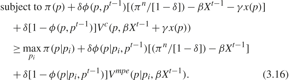
Finally, let us explore the impact of the discount factor on the collusive price path when (3.16) binds. In the standard collusive model without competition law and enforcement, the collusive price is increasing in δ when the equilibrium condition is binding, because more-patient firms have a weaker temptation to cheat; they prefer to maintain future collusive profits rather than to increase current profit by cheating. That force is operative here as well, but there is a second role for time preferences. The cartel faces an intertemporal trade-off in that a higher price in the current period raises current profit but lowers the future payoff by increasing both the likelihood of detection and the size of the penalty. As cartel members become more patient, they prefer not to raise the collusive price as fast. As depicted in figure 3.1, a higher discount factor can initially lower the collusive price path but also raise the steady-state price (for the usual reasons) which then means the price path is eventually higher.

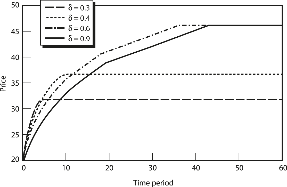
Figure 3.1
Effect of the discount factor on equilibrium price path.
Source: Harrington (2004a).

The preceding result is shown numerically in Harrington (2004) and a related result is proven in Houba, Motchenkova, and Wen (2012) for a simpler model. They show that as δ goes to one, the optimal cartel price goes to the static Nash equilibrium price. The model is the infinitely repeated Bertrand price game, but the probability of detection is linear in contemporaneous price and the penalty is proportional to contemporaneous profit. Thus, there are no state variables. In the event of conviction, the cartel is permanently shut down with probability ζ and remains active with probability 1 − ζ (in which case, it could be convicted again in the future). The best symmetric equilibrium price is characterized assuming the grim punishment.

If ζ = 0, then the standard result emerges, which is that the collusive price is (weakly) increasing in δ. However, if ζ > 0, then the collusive price converges to the static Nash equilibrium price as δ goes to one. When δ is low, a collusive equilibrium does not exist. When δ is intermediate, there is a collusive equilibrium, and the price is set at the highest level satisfying the equilibrium condition. When δ is high, the equilibrium condition is not binding, in which case the cartel sets price at the unconstrained joint profit-maximizing price, which is decreasing in δ due to competition policy. As firms are more patient, they become more concerned about being detected (and permanently shut down), so they limit how high is the price, because the probability of detection is increasing in price. As δ → 1, they are content to set price arbitrarily close to the competitive price to ensure a long stream of (low) collusive profits.

3.3.3   Dynamic Game with State Variables: Endogenous Detection Technology

While these dynamic models are a useful advance, a problem is the lack of richness in modeling how the price path impacts detection. The approach is black box, in that an exogenous function is specified whereby the probability of detection depends on the price path (such as the contemporaneous price level or price change). A more foundational approach would be to model a buyer or CA as a player and characterize an equilibrium in which a buyer or CA is trying to determine whether a cartel exists and, at the same time, the cartel is trying to avoid detection. While this approach has been pursued in a static setting (which is reviewed in section 4.2), it poses a serious technical challenge in the dynamic setting.

A step in that direction was taken in Harrington and Chen (2006). Rather than model a buyer as an optimizing player, they are viewed as empiricists. A cartel is detected when a buyer becomes suspicious, which is presumed to occur when observing a price path that is unlikely to be based on the history of prices. The idea is that an anomalous price path triggers detection and what is anomalous depends on what buyers have come to expect.

Suppose that firms have a common and stochastic linear cost function C^t(q) = c^tq. c^t is a random walk, c^t = c^t−1 + ε^t, and and is iid. Absent collusion, cost shocks provide a competitive rationale for large price increases. Buyers have the null hypothesis that firms compete and will reject the null when the price series is sufficiently unlikely. The prior information of buyers is that price is a random walk p^t = p^t−1 + η^t, where η^t ∼ N(?, ?) is normally distributed, but buyers do not know the moments of the distribution on η^t. In forming beliefs on those moments, buyers use past price changes, and it is assumed they have a finite memory of k periods, so their data set is {Δp^t−k, . . . , Δp^t−1}, where Δp^τ ≡ p^τ − p^τ−1. Using the sampling moments, buyers’ distribution on Δp^t is , where

To limit the dimensionality of the state space, buyers’ sampling moments are approximated by the equations of motion:

Buyers will assess the reasonableness of recent price changes by testing a sequence of the z(<k) most recent price changes. Given their beliefs on Δp^τ, the likelihood of these z price changes is specified to be a “moving” likelihood, , where f is the normal density function. The maximum likelihood for the z most recent price changes is

A buyer’s suspicions about collusion is assumed to depend on the relative likelihood assigned to those recent price changes:

The movement of L^t is approximated by the equation of motion,

Finally, the probability of detection ϕ(L^t) is assumed to be a decreasing function of L^t. In sum, the less likely buyers find recent price changes (based on the history of price changes), the more likely they are to conclude there is collusion. Such an event suggests a change in the price-generating process, and the presumption is that buyers would conclude one explanation is a change in conduct due to cartel formation.

This detection technology is embedded in an infinite-horizon oligopoly price setting, where the state variables are the lagged price, the lagged cost, the accumulated penalty, the sampling moments, and the likelihood. The cartel’s dynamic problem (when equilibrium conditions are not binding) is numerically solved for the policy function that prescribes the optimal price depending on the state variables. To produce simulated price paths, the model is run for 40 periods when firms are competing, so that buyers can form prior beliefs on the competitive pricing process. A cartel is created in period 41, and it inherits the state variables coming out of the competitive phase.

Figure 3.2 shows two typical price paths and includes the noncollusive (or competitive) price path as a benchmark.¹⁸ The collusive price path has a transition phase and then a stationary phase. During the transition phase, price steadily rises, somewhat independent of cost shocks. In the stationary phase, price varies with cost but, notably, the collusive price path is less variable than the competitive price path. This is shown more systematically in Harrington and Chen (2006), where, for a large number of simulated price paths, the variance of prices over time is found to be significantly lower when firms collude. The low price variability under collusion is due to the cartel’s desire to avoid triggering suspicions by making large price changes. If cost changed significantly (and cost is not observed by buyers), the cartel will want to avoid changing price too much. Even though suspicions would arise for the wrong reason—the big price change is due to cost shock and not a change in conduct—any suspicions could trigger an investigation.¹⁹

Figure 3.2
Collusive and noncollusive price paths.
Source: Author.

3.3.4   Collusive Equilibria with and without Communication

The previous models presume that any collusive equilibrium is unlawful. Thus, if firms choose to collude, they were assured of facing the prospect of penalties. However, as described in chapter 1, not all collusion is illegal. If firms decide they want to try to shift the industry from competition to collusion, there is still the decision regarding how to consummate and conduct collusion and whether to do so in an unlawful manner. Of course, it must be the case that lawful collusion is less effective than unlawful collusion; otherwise, firms would always pursue the legal variety. As only collusion involving certain forms of communication is illegal, firms can then either seek to most effectively collude by engaging in communication practices that are illegal or pursue less effective means of communication (or not communicate at all) and thereby avoid the prospect of conviction and paying penalties.

In the context of this book, the relevant question is: When does competition policy induce firms to choose collusion with less effective means of communication, and how does it change the form of collusion? To my knowledge, there are only two papers that speak to that question, though a growing (though still small) body of research characterizes collusion with communication, and some of it examines when collusion is more effective with communication. That research is likely to provide the foundation for then introducing competition policy and assessing its impact on collusion.

Firms are assumed to have private information on their costs in Athey and Bagwell (2001, 2008) and on demand in Gerlach (2009); they use costless messages (that is, “cheap talk”) to possibly convey that private information and thereby coordinate on a more efficient outcome for the cartel. There is a second strand of research in which firms’ sales or some other endogenous variable is private information and firms exchange messages for monitoring purposes. This line encompasses Aoyagi (2002), Harrington and Skrzypacz (2011), Spector (2015), and Awaya and Krishna (2016). Chan and Zhang (2015) model the exchange of messages when firms’ costs and sales are both private information.

Our focus here is on the subset of this literature comparing collusion with and without communication in order to assess the efficacy of communication and thereby provide insight into when firms want to communicate and possibly unlawfully collude. While it seems obvious that communication will make collusion more effective, the challenge is twofold in proving it. First, communication is useful only if the messages are truthful and that requires creating the right set of incentives for firms to accurately communicate. Second, many clever and complicated ways can be used to structure equilibria without communication, which makes it difficult to characterize the maximal equilibrium payoff and thereby determine whether equilibria with communication can result in higher payoffs.

Athey and Bagwell (2001) consider a standard infinitely repeated game with perfect monitoring when firms’ costs are iid and are private information. They compare collusive equilibria with and without cheap talk messages, where the intent of these messages is to share information about cost in order to enhance industry profit. A first-best solution requires the firms with the lowest cost in that period to supply the market, but achieving that outcome requires sharing private information about their costs, and each firm has an incentive to report that its cost is low in order to be able to supply. It is shown that firms can be induced to provide truthful messages by trading market shares over time. Though a firm is less likely to be allocated any market share if it announces it has high cost, it is compensated with a higher market share in the future, which is more valuable in expectation, as it may have low cost at that time.20

Awaya and Krishna (2016) and Spector (2015) examine an imperfect monitoring setting in which firms’ prices and sales are private information and firms’ realized sales are stochastic. The objective is to understand when sharing information about sales is valuable in the sense that there is an equilibrium when messages are used that yields a higher payoff than the highest equilibrium payoff when messages are not used. The compliance challenge is that a firm may undercut the collusive price, realize large sales, and (inaccurately) report that its sales are not large.

In the case of Awaya and Krishna (2016), if cheap talk messages are not used, then the environment is one of private monitoring; that is, each firm must decide whether to continue to charge the collusive price based only on what it knows about its own sales. When firms are sufficiently patient and monitoring is sufficiently noisy, there exists an equilibrium with cheap talk messages that is strictly more profitable than any equilibrium in which firms do not communicate. The equilibrium with communication has firms self-report sales and impose a punishment if those reports are not sufficiently similar. To deliver that result, a necessary condition on firms’ demand functions is that firms’ sales are highly correlated but only when their prices are similar. Hence, if all firms set the common collusive price, then their sales will be highly similar. In that situation, the submission of an inaccurate sales report is easily detected, because firms’ sales reports will fail to be nearly identical. However, when a firm deviates from the common collusive price, firms’ sales are not strongly correlated (by assumption), which implies that the deviator’s sales are not very informative of other firms’ sales. This means it is unlikely to submit a report that is similar to those of the other firms and, therefore, a punishment is likely. In sum, firms find it optimal to price at the collusive level and truthfully report their sales which means monitoring is more effective when firms communicate their sales to one another.

Spector (2015) considers a similar situation but where each firm privately learns its sales at a high frequency (e.g., monthly) and all firms’ sales are publicly revealed at a low frequency (e.g., annually). Thus, perfect monitoring occurs on a low-frequency basis, and the issue is whether firms can do better by providing reports of their sales as soon as they learn them and conditioning their prices on those reports. Keep in mind that the self-reports have to be incentive compatible, while the public reports are assumed to be factually correct. Sufficient conditions are provided for an equilibrium to exist in which firms more effectively collude by self-reporting their high-frequency sales information. The tension here is that if firms use the public reports of sales, inefficiencies are reduced because of less noise, but then punishment is delayed. However, if firms truthfully share those private signals through cheap talk messages, then they can have precise public signals at high frequency. Furthermore, it is incentive compatible to report accurately, because a misleading sales report will later be revealed by the public signal and, at that time, would be harshly punished. In equilibrium, that punishment is not used, so the threat is costless. In sum, both Awaya and Krishna (2016) and Spector (2015) show that firms reporting their sales to one another yields higher profit, which suggests a set of circumstances in which firms may prefer to collude unlawfully.²¹

There is a distinction between communication that serves to move firms from a noncollusive to a collusive equilibrium and communication that is part of a collusive equilibrium and acts to make collusion more effective through information sharing. Generally, the law is concerned with the former variety, but the latter is often part of evidence in proving liability. The research described thus far involves communication that is part of an equilibrium for the purpose of delivering more effective monitoring.

Encompassing communication for the purposes of coordinating on collusive strategies motivates the analysis in Harrington (2017). Though not part of the model, the presumption is that firms have constrained their ex ante communication to avoid acting illegally, and the implication is that they lack common beliefs about their collusive strategies. The focus is on a price leadership scheme, whereby it is common knowledge that price increases will be matched (and failure to do so results in competitive prices) but there is a lack of mutual beliefs regarding who will lead on price, at what level, and at what time. Thus, there is partial mutual understanding with regard to collusive strategies. Sequential rationality is assumed to be common knowledge. Two questions are addressed: (1) Are these mutual beliefs sufficient to result in supracompetitive prices? and (2) If they can achieve supracompetitive prices, are those prices less than what would be achieved if there were a mutual understanding of the strategy profile (as presumed by equilibrium)?

In answer to the second question, it is shown that there is an upper bound on price that is strictly less than the maximal equilibrium price (using the same punishment). Without mutual beliefs regarding the collusive price, coordinating on a higher collusive price requires some firm to take the lead in raising price. What is constraining how high price can go is the trade-off a firm faces when it acts as a price leader: It forgoes current demand and profit in exchange for higher future profit when rival firms raise their prices to match its price increase. This constraint on price is to be contrasted with equilibrium, where what limits the price is the condition that a firm finds it unprofitable to undercut it. Partial mutual understanding makes the coordination on price the constraining factor, not the stability of the price that is eventually agreed on. With regard to the first question, if firms engage in Bayesian learning regarding other firms’ strategies and their prior beliefs have full support, then supracompetitive prices will eventually occur for sure.²²

The research described thus far does not encompass competition law and enforcement. That is done in Mouraviev (2013) while taking a black box approach to communication. The imperfect monitoring structure of Green and Porter (1984) is modified to allow firms, in each period, to meet to exchange verifiable information as to their realized quantities. If firms unanimously decide to meet, then for that period, an imperfect monitoring setting is converted into a perfect monitoring setting. The cost of doing so is that collusion is now presumed to be unlawful, given that firms met and exchanged their sales information. The cartel then faces a trade-off when it comes to structuring the collusive equilibrium, because having meetings enhances monitoring, which serves to make deviations less profitable but also reduces the collusive value (because of the expected penalty).

Each period has three stages. In stage 1, after observing the previous period’s price, firms simultaneously decide whether to meet and exchange (in a verifiable way) the previous period’s quantities. If all firms agree, then they meet and there is perfect information disclosure. In stage 2, firms choose quantities, and a common price is publicly observed, which depends on the sum of all firms’ quantities (as the product is presumed homogeneous) and a demand shock. At this stage, the current period’s quantities are private information. The inference problem is that a low realized price could be due to a low demand shock or because some firm did not comply with the collusive outcome and overproduced. In stage 3, if firms met in stage 1, then the industry is investigated with probability σ, in which case a fixed penalty of F is levied.

The optimal perfect public equilibrium involves specifying a trigger price ρ (which lies in the equilibrium support of price when all firms produce the collusive quantity) such that if the realized price (1) is above ρ (and below the upper bound of the equilibrium support), then there is no meeting and firms produce the collusive quantity; (2) is below ρ and above the lower bound of the equilibrium support, then there is a meeting, and firms produce the collusive quantity if it was revealed that no firm deviated and punish otherwise; and (3) falls outside the equilibrium support, in which case there is punishment. Comparing this equilibrium to when firms do not have the option to exchange verifiable information on their sales, price wars (in the sense of Green and Porter 1984) do not occur and are replaced with “meetings” in equilibrium. Thus, the predicted price series is very different. It is also shown that, when the expected penalty is sufficiently low, the best equilibrium with meetings yields a higher value than the best equilibrium without meetings.

Mouraviev (2013) generates the finding that price wars are more common when cartels are illegal. If there is no competition policy, then in the context of the model, colluding firms will always meet to exchange sales information and avoid price wars. If there is a CA with sufficiently severe penalties at its disposal, then the preferable equilibrium for the cartel may be the one without meetings, which then implies the usual price wars of Green and Porter (1984).

A related approach is taken in Garrod and Olczak (2016a) though in a different informational setting with a distinct set of findings. The oligopoly structure is a capacity-constrained price game with homogeneous goods, and firms are allowed to have different capacities. Market demand is perfectly inelastic at m units, where m is stochastic, iid, and not observed by firms. A firm’s price (and its realized quantity) are private information. Without communication, there are no public signals, so this is a private monitoring setting.²³ There is an inference problem when it comes to sustaining collusion, because low sales for a firm could be due to a rival firm’s deviation or low market demand. The optimal perfect public equilibrium has periodic reversion to the static Nash equilibrium when a firm’s quantity falls below some threshold. (By clever construction of the model, it is common knowledge among firms when to punish, even though there is no public signal.) A crucial feature of this equilibrium is that, when the smallest firm is smaller (in terms of capacity), then the frequency of punishment becomes greater, because it is more difficult to detect a deviation. A firm that deviates from the collusive price has demand exceeding its capacity and, assuming that a firm supplies enough to meet all its demand, its output equals its capacity. Hence, the smaller a firm is, the smaller will be the reduction in other firms’ demands as a result of that deviation which, roughly speaking, makes monitoring more challenging, and that manifests itself in more frequent punishments.

The next step is to characterize equilibrium with communication. After prices are set and quantities and profits are privately observed, each firm decides whether to provide verifiable information to the other firms regarding the price it charged that period.²⁴ Equilibrium has firms charging a collusive price and then sharing information on their prices. A punishment ensues if the reported price is not the collusive price or a firm fails to report price. In equilibrium, there is no punishment (which is in contrast to when firms do not communicate). However, communication among firms results in a probability each period that the cartel is detected and penalized, where a firm’s penalty is proportional to its capacity. Note that firms did not choose to communicate every period in Mouraviev (2013), while here communication takes place every period.

One of the central objectives is to determine when firms find it more profitable to collude unlawfully by communicating. Unlawful collusion avoids ever having to punish but comes with an expected penalty. If the number of symmetric firms decreases, then, holding industry capacity fixed, the smallest firm becomes larger. This makes collusion without communication more profitable, because punishments are triggered less frequently. Hence, unlawful collusion is less likely when there are fewer firms, because firms choose to collude without sharing information about prices. One interpretation of this finding is that tacit collusion substitutes for explicit collusion when there are fewer firms.

3.4   Summary of Findings

In summing up some of the findings, it is useful to think about them in the context of addressing two sets of questions. First, to what extent does the presence of competition law and enforcement change our understanding of collusion? How does the constraint imposed by the prospect of conviction and penalties affect collusive behavior? Are unlawful cartels predicted to operate differently from lawful cartels? Second, what is the impact of competition law and enforcement and, in particular, does it have the desired effect of lowering the collusive price, shortening cartel duration, and reducing the extent of cartel formation? Under what conditions is competition law and enforcement ineffective or even counterproductive?

In these models, competition policy is represented by the probability of conviction and the magnitude of the penalties inflicted on those convicted. Its impact on the presence of collusion can be direct when it involves discovering, prosecuting, and convicting a cartel, which then causes collusion to terminate either temporarily or indefinitely. These theories also flesh out the indirect effect of competition policy. The prospect of premature termination of collusion and the paying of penalties lowers the collusive payoff, which then impacts the equilibrium conditions. This effect could be so large that collusion is no longer an equilibrium, and therefore, cartels are deterred. But even if a cartel is not deterred, competition policy’s influence on the equilibrium conditions can make cartels less stable in the sense that there is a wider set of market conditions in which equilibrium conditions are not satisfied, so that the cartel collapses. This enhanced instability translates into shorter cartel duration. A lower collusive payoff—due to shorter duration (because of shutdown by the CA or internal collapse) and higher expected penalties—may tighten the equilibrium conditions which then requires firms to set a lower collusive price if compliance is to be ensured.

Katsoulacos, Motchenkova, and Ulph (2015a) classify these three effects of competition policy as the direct effect from shutting down active cartels, the indirect-deterrence effect of deterring cartels from forming, and the indirect-price effect of constraining the price charged by the cartel that still forms and remains active. The theories discussed above also point out that competition policy affects the payoff to deviating, and it is possible that a more aggressive competition policy could lower the deviation payoff more than the collusive payoff (in which case the equilibrium conditions are loosened, which makes collusion easier). One must then be careful in assessing how competition law and enforcement affects the environment for collusion.

With regard to cartel birth, death, and duration, theories have generally shown that a higher rate of discovery and conviction and higher penalties have the desired effect of cartels forming in fewer markets and with shorter duration, which translates into a prediction of a smaller fraction of markets that are cartelized. Regarding cartel membership, the presence of competition policy alters the “all are welcome” policy of legal cartels. In the absence of competition policy, a cartel would always prefer a firm to be in the cartel rather than outside it, where it would undercut the collusive price and not constrain its output. However, concerns over detection can result in a cartel limiting its membership. Competition policy is then reducing the size of the largest stable cartel, which has the beneficial impact of reducing the collusive price. At the same time, the tightening of the equilibrium condition because of competition policy may increase the size of the smallest stable cartel.

The theory of collusion under competition law and enforcement has resulted in a rich set of new findings when it comes to pricing. Less dispersion of collusive markups is predicted when the cartel is illegal than when it is legal, because competition policy deters cartels with low markups from forming and constrains the markups of those that do form. Though competition policy often limits the collusive price, if the equilibrium conditions are not binding and the penalty is not sensitive to the price charged, then the steady-state collusive price is unaffected by the presence of a CA. Furthermore, if the equilibrium condition binds, it is even possible for the collusive price to be higher under competition policy, because it serves to lower the deviation payoff more than it lowers the collusive payoff. However, those conditions seem rather special.

Where the theories have yielded richer findings is in characterizing price dynamics. With standard theories of collusion, a legal cartel probably has no reason not to raise price significantly upon cartel formation.25 But if the cartel is illegal and detection is sensitive to the price path, then the cartel may choose to raise price gradually. Broadly consistent with some actual cartels, the price path has a transition phase, in which price rises in a manner largely independent of cost shocks and is followed by a stationary phase where price is less sensitive to cost shocks than under competition. It may also be the case, however, that if competition policy discourages meetings among colluding firms, this could result in price wars that would not occur if collusion was legal. A fundamental finding in the standard theory of collusion is that the equilibrium price is weakly increasing in firms’ discount factors. Competition policy alters that comparative static, because a higher discount factor can result in initially lower prices though, as with lawful cartels, it raises the long-run price.

Notes

1.  The ensuing analysis is from Harrington (2014).

2.  It is straightforward to adapt the ensuing analysis to allow the cartel to reform with some probability. Also, one could allow σ to vary over time; see Hinloopen (2006).

3.  It is immediate that Ψ(σ, f, β) is increasing in f and β. A sufficient condition for Ψ(σ, f, β) to be increasing in σ is σ ≤ 1/2 which is a necessary condition for collusion to be stable; that is, if σ > 1/2 then (3.4) does not hold.

4.  For example, Selten (1973), Prokop (1999), and Kuipers and Olaizola (2008).

5.  For some progress on this topic, see Paha (2013).

6.  One can get “collapse” (in the sense that there are no collusive equilibria) with the Bertrand price game but, essentially, it is a special case of the Prisoners’ Dilemma, where π^d = nπ^c and πⁿ = 0.

7.  Examples can be found in Harrington (2006), Connor (2008), and Marshall and Marx (2012).

8.  Also see Bartolini and Zazzaro (2011) and Kalb (2016).

9.  For a theoretical and empirical analysis of collusive pricing dynamics due to uncertainty about cartel stability, see Chilet (2016).

10.  Having enriched the setting beyond the Prisoners’ Dilemma, there are then many continuation equilibria associated with a deviation. For simplicity, I focus on the grim punishment, though the results to be discussed are generally robust to the equilibrium selection.

11.  One way to motivate low markups is to augment the model so that there is a perfect substitute for this good outside this market that sells for > pⁿ. This implies the collusive price cannot exceed (for if it did, then all consumers would turn to buying the substitute good). For markets in which is close to pⁿ, the collusive price will be and the markup will be low.

12.  Of course, this is an expectation, so that an illegal cartel would not form if the markup was expected to be small. If there is uncertainty about what markup is stable, then the realized markup could be small.

13.  There is a related finding in Jensen and Sørgard (2014), where it is shown that penalties tend to cause the incentive compatibility constraint (determining the collusive price) to bind for cartels able to produce large overcharges, and for the participation constraint (determining whether collusion is profitable) to bind for cartels only able to produce low overcharges.

14.  Chen and Harrington (2007) and Bos, Peeters, and Pot (2013) also show how competition policy can have perverse effects by promoting collusive behavior.

15.  For an early paper on the dynamics of collusive pricing when there is the threat of prosecution, see Levy and Rodriguez (1987).

16.  The ensuing analysis is based on Harrington (2003, 2004a, 2005).

17.  In equilibrium, all firms charge the same price, so the summary statistic is that common price.

18.  As the noncollusive price path is an affine function of cost, it also shows how cost is moving over time.

19.  A discussion of this theory and other research in the context of screening for cartels is provided in Harrington (2007, 2008a).

20.  For the model of Athey and Bagwell (2001), Hörner and Jamison (2007) show how almost first-best payoffs can be achieved without communication. That paper speaks to the statement made earlier that there are many clever and complicated ways to effectively collude without sending messages.

21.  Also see Escobar and Llanes (2016), which shows the value of communication about private information on market conditions in the context of collusion.

22.  The proof uses a result of Kalai and Lehrer (1993), though it is not subject to the criticism of their “grain of truth” assumption, because, given the other assumptions on firms’ prior beliefs, the support is a countable set.

23.  Equilibrium without communication was originally characterized in Garrod and Olczak (2016b).

24.  It is shown that results are robust to not assuming verifiable information but instead having the price report be cheap talk, in which case an incentive compatibility constraint must be satisfied for it to be truthful. However, the proof of robustness relies heavily on the special assumptions made on demand and capacities.

25.  A caveat to that statement is that a cartel may want to keep itself hidden to affect bargaining with industrial buyers. Buyers may be more willing to accept a large price increase if they think it is due to higher cost than to a change in firm conduct; see Kumar et al. (2015) and Kumar (2016).