CHAPTER TWELVE

Option Pricing

Understanding how options are priced is essential for serious investors—even if they are going to rely on computer models to do the actual pricing. The reason investors need to understand option pricing is that it is the key to:

• Establishing and maintaining valid hedges that use options
• Doing relative value analysis between different options, and options vs. the underlying
• Understanding the option sensitivities
• Understanding the various option strategies
• Understanding long-dated options like LEAPS (Long-term Equity Appreciation Securities) and warrants
• Understanding convertible bonds/reverse converts and other debt equity hybrids

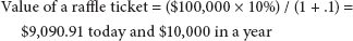
For the purposes of pricing, options are raffle tickets. Like all raffle tickets, their value is:

Value of a raffle ticket = PV (potential prize × probability of winning)

EXAMPLE ONE

Prize $100,000, 10 tickets sold, winner announced in a year, interest rate 10%

When this model is translated to options, you find that:

• The potential prize equates to the intrinsic value at expiration.
• The probability of winning equates to the probability that the option will be in the money at expiration.

LOGNORMAL DISTRIBUTIONPRICING MODEL

To estimate whether there will be any intrinsic value at expiration (and if so, how much) requires building a model. As with all pricing models, the more assumptions its designers make, the simpler the model is to build. The lognormal distribution pricing model includes a number of assumptions:

Continuous trading— The assumption that the underlying instrument trades continuously (24 hours a day, 365 days a year) is reasonable for some underlying instruments, like the major currency pairs (EUR/USD, JPY/USD, GBP/USD), major commodities (oil, gold), and major stock indices (S&P 500, FTSE 100). The assumption is not reasonable for a thinly traded OTC stock—and so neither is the lognormal distribution pricing model.

Infinite infinitely small price moves— The assumption that the price of the underlying changes in an infinite number of infinitely small price moves is not strictly true for any underlying. It is reasonably true for very liquid underlying instruments where the bid-ask spread is tiny relative to the price of the underlying and large trades do not cause price jumps.

Underlying price reflects all known information— The model assumes that the price of the underlying accurately reflects all known information. Since the current price reflects all known information, the only thing that causes the price to change is new information—which is, by definition, unknown. Since this new information is random, the underlying’s price movements in the future will be random.

Past prices do not impact future prices— If this assumption is true, then the entire field of technical analysis is worthless. It has been demonstrated that technical analysis adds value at least over the short term, so the lognormal pricing distribution model is only good for options that have more than a month left until expiration.

Past volatility indicates future volatility— The lognormal pricing distribution model assumes that past volatility of a stock is indicative of future volatility. If the market has trouble reaching a consensus on what the future earnings of a company will be or how available a commodity will be, the price of the stock or commodity will be volatile as the market reacts and overreacts to each new piece of information. Also, a lack of consensus often results in the stock or commodity being held in “weak hands” that will reverse their position with each news announcement.

Future returns are normally distributed— Here the assumption is that the distribution of future returns, not future prices, is normally distributed. If the future prices were normally distributed, that would create two problems:

• First, if the stock was currently selling for $100 and the distribution 1 year from now was normally distributed around $100, there would be an equal probability of a gain and a loss. Also, the magnitude of the potential gains would equal the magnitude of the potential losses. If the size of the gains and losses is the same, and the probability of gain and loss is the same, the potential gains and losses in a year are equal. However, when you factor in transaction charges, both longs and shorts must lose over the long term. This is not a model for investing; it is the model that built Las Vegas.
• Second, suppose that the mean was $100 and the standard deviation was $40. In this case the distribution of future prices would look like the one depicted in Figure 12.1. The problem is that this distribution includes negative values, which are impossible for stocks, bonds, and commodities.

FIGURE 12.1

Normal Distribution

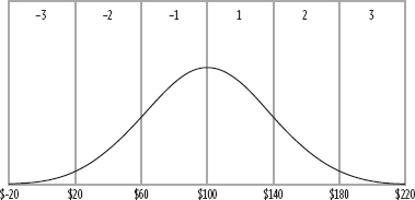
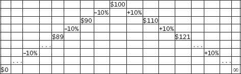
If, however, we assume that the returns (instead of the prices) are normally distributed, then 10% gains and 10% losses are equally likely—as are two successive 10% gains and two successive 10% losses. In this event, a $21 gain has the same probability of occurring as a $19 loss. Ten percent gains, ad infinitum, cause the price to approach infinity, while 10% losses, ad infinitum, cause the price to approach $0. Both are consistent with what we know about the possible price range of stocks and commodities, as you can see in Figure 12.2.

FIGURE 12.2

Impact of Successive Fixed Percent Gains and Losses

Risk-free rate is both known and fixed— The risk-free rate is a concept. In the US, the Treasury spot rate serves as a reasonable surrogate. Even though Treasuries have some credit risk, it is minimal so that the error introduced is negligible. However, the Treasury spot rates are not fixed, but as they change so will the value of the option.

Everyone can borrow and invest at the risk-free rate— While everyone can invest at the Treasury rate, not everyone can borrow at the risk-free.

Finally, the lognormal pricing distribution model assumes that:

• There are no transaction costs.
• There are no dividends.
• Option has European expiration.
• Life of the underlying cannot be changed due to call, put, merger, etc.
• Delivery process is fair and unbiased.

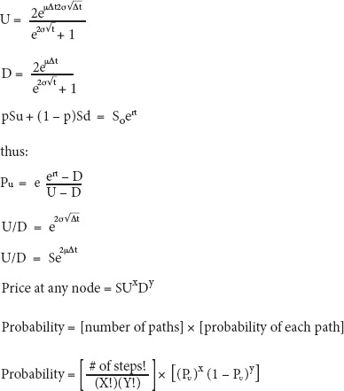
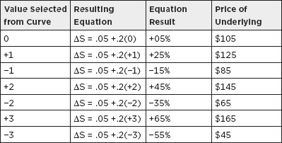
Given these assumptions, the formula that explains the behavior of the underlying is:

ΔS = μΔt + σε√Δt

S = the stock’s price

μ = the risk-free rate

σ = the stock’s volatility

ε = normal curve with a mean of 0 and standard deviation of 1

t = time until expiration

EXAMPLE 1

Market value = $100

Strike price = $100

Volatility = 20%

Expiration = 1 year

Risk-free rate = 5%

ΔS = .05(1) + .2ε(1)

ΔS = .05 + .2ε

This equation is then solved a “statically infinite” number of times. To solve the equation a value is selected at random from a standardized normal curve (mean = 0, standard deviation = 1). Naturally, the value “0” and values close to it will be selected most often. As with any normal curve, the probability of randomly selecting a result between:

• 1 and −1 standard deviations is approximately 67%
• 2 and −2 standard deviations is approximately 96%
• 3 and −3 standard deviations is approximately 99+%

Also, the probability of randomly selecting a value of +1 standard deviations from the mean is equal to the probability of randomly selecting a value of −1 standard deviations from the mean. The information presented in Figure 12.3 depicts the results of selecting random values and plugging them into the equation in order to estimate the future price. (Note that only whole numbers were used; in practice, numbers would be selected out to 4 to 6 decimal places.)

FIGURE 12.3

Price of Underlying

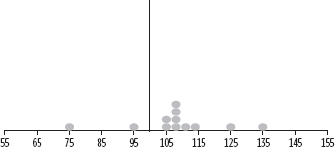
The results (the possible future prices) are then plotted. As more and more results are added, the stacks start to grow; the dots become smaller and then coalesce, as shown in Figure 12.4.

FIGURE 12.4

Start Plotting the Results

As the number of results added to the graph is increased, the shape of the distribution of future prices becomes clearer and clearer (see Figure 12.5 and Figure 12.6).

FIGURE 12.5

Continue Plotting the Results

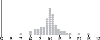
FIGURE 12.6

Continue Plotting the Results

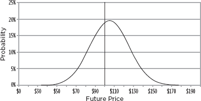
As the number of results increases, the shape becomes smoother and eventually you end up with a lognormal distribution of possible prices in a year, as shown in Figure 12.7. Because the assumption that the price changes in an infinite number of small price changes was made up front, the resulting curve is continuous. Note that because the curve is lognormal, there is a bias toward the upside. The average move up exceeds the average more down. The probability of an up move also exceeds the probability of a down move.

FIGURE 12.7

Resulting Lognormal Curve

The advantage of having a continuous curve is that it makes it simple to answer the questions that need to be answered to value the options; namely:

• What will the option’s intrinsic value be at expiration?
• What is the probability that the option will have any intrinsic value at expiration?

The intrinsic value at expiration for an at-the-money $100 call would be MV − $100. Thus, in a year, if the stock is selling for:

• $101, the intrinsic value would be $1
• $102, the intrinsic value would be $2
• $105, the intrinsic value would be $5
• $110, the intrinsic value would be $10
• $150, the intrinsic value would be $50

It is impossible to know, in advance, what the intrinsic value will be. However, we do know what the probability is that the intrinsic value will be $1, $2, $3,…$50,…$70,…etc.

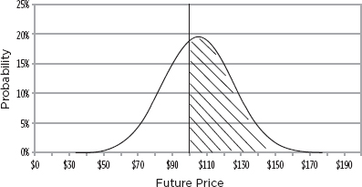
Since the probability of each intrinsic value is known, we can calculate a weighted average of the various possible intrinsic values. This weighted average can be expressed as a multiple of the spot price. This multiple, is called the “up factor” (U). This is the “average” amount by which the S price will rise over a time frame given its volatility. Of course, the price could rise by more, rise by less, or not rise at all. Multiplying S and U together produces the weighted average (weighted by probability) of all the prices higher than the spot price.

In Figure 12.8, $122.14 is the weighted average of the shaded region.

FIGURE 12.8

Weighted Average of Higher Prices

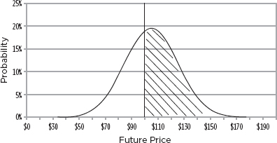
The weighted average of the prices that are lower than spot can be found by calculating the “D” factor and multiplying it by spot.

Note that while the average up move is $22.14, the average down move is $18.13. This is because of the upward bias inherent in a lognormal distribution. It is also one of the reasons why an ATM call has a greater value than an ATM put.

FIGURE 12.9

Weighted Average of Lower Prices

The second question, what is the probability that the call or put option will be in the money can be answered by solving for the probability up (P_u). The U and D are the same as we discussed earlier. Once the probability of an up move is calculated, the probability of a down move (P_d) is simply: 1 − P_u.

These four numbers (U, D, P_u, and P_d) are a shorthand way of describing the entire lognormal curve and are all that is necessary to value ATM options. (See Figure 12.10 and Figure 12.11.) Consider the following:

Value of a raffle ticket = PV (potential prize × probability of winning)

Value of an ATM call = PV (average intrinsic value above spot × probability of up move)

Value of an ATM put = PV (average intrinsic value below spot × probability of down move)

FIGURE 12.10

Probability of Price Going Up

FIGURE 12.11

Calculation of ATM Call and Put

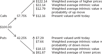
Starting at $100, if the stock goes up, it will go up (on average) to $122.14. That means the average intrinsic value at expiration (the average “win”) is $22.14. Of course, there is only a 57.75% chance of having a winning ticket, thus the option is only worth $12.79 (weighted average intrinsic value × probability of up move) in a year. It is worth the present value of $12.29 today − (12.79^{e -.05}) = $12.16.

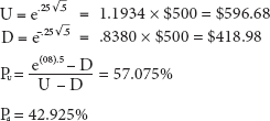
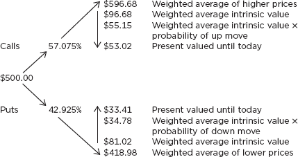
As another example, suppose Palladium is selling for $500, its historic volatility is 25%, and the risk-free rate is 8.00% cc 30/360. Let’s price the 6-month ATM call and put, as shown in Figure 12.12. Going right to the calculation of the four values that abbreviate the entire lognormal curve:

FIGURE 12.12

Calculation of ATM Call and Put

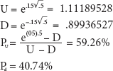
As a final example, suppose the current risk-free rate is 5.00% cc 30/360 and its annual volatility is 15%. Use this information and the equations that follow to determine the price of an ATM 6-month call and put. (See Figure 12.13.)

FIGURE 12.13

Calculation of ATM Call and Put on Rates

BINOMIAL MODELS

The problem with the lognormal distribution model is that, while it can be used to value options on stocks, commodities, or interest rates, it can only value ATM options. The only data the model generates is the probability of up moves and down moves from spot. The only intrinsic values are measured from spot.

Investors want to value options across a broad range of strike prices—not just ATM options. To do this, they need to break time down into smaller intervals. By doing so, the binomial model generates more data that can then be used to value any option.

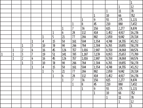
With time broken into smaller intervals, a price tree can be built, as shown in Figure 12.14. U and D are calculated as before—but just with a shorter time frame. The price at each node in the tree is simple: the spot price times the number of U factors and D factors to reach the node.

FIGURE 12.14

The Price Tree

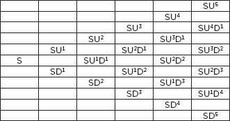
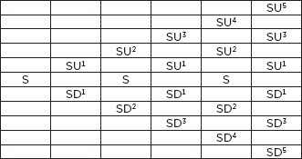
However, since U times D = 1, the tree simplifies to the one shown in Figure 12.15, where the values along the edge are replicated in the interior.

FIGURE 12.15

The Simplified Price Tree

The probability of reaching a node in the tree is equal to the probability of each path that leads to that node times the number of paths that lead to that node.

• The probability of each path that leads to the node is determined using P_uXP_dY, where:
• P_u equals the probability of an up move
• P_d equals the probability of a down move
• X equals the number of up moves to reach the node
• Y equals the number of down moves to reach the node
• The number of paths that lead to a node is equal to:

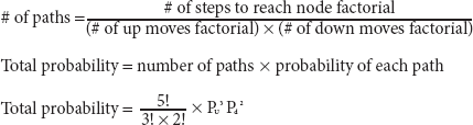
Thus, the probability of reaching the 2 node down on the fifth step (see Figure 12.16) would be calculated:

Total probability = number of paths × probability of each path

The total probability of reaching each node is:

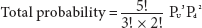
FIGURE 12.16

The Probability Tree

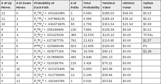
If the option has a European expiration, the only values needed to value the option are the last values in the tree. These are the ones to the far right and are referred to as the terminal values.

EXAMPLE PRICING EUROPEAN OPTION USING THE TERMINAL VALUES OF A BINOMIAL MODEL:

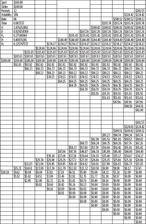
Spot = $100

Strike price = $130

Expiration = 1 year

Steps = 12

Annual volatility = 18%

Risk-free rate = 6.00%

Calculate the four lognormal curve surrogates:

In the case in Figure 12.17, the top four values are in the money for a 130 call. Multiplying the total probability of reaching these nodes by the intrinsic value at these nodes gives the value of all four options. Summing them and calculating the PV of the result gives us the value of the call option.

In the case in Figure 12.18, the bottom nine values are in the money for a 130 put. Multiplying the total probability of reaching these nodes by the intrinsic value at these nodes gives the value of all nine options. Summing them and calculating the PV of the result gives us the value of the put option, as shown in Figure 12.18.

FIGURE 12.17

Using Terminal Values to Value Options

FIGURE 12.18

Terminal Values Used to Value Put

RELATIVE VALUE OF AMERICAN VS. EUROPEAN OPTIONS

American and European options can either have the same value—or different values—depending on the type of option and whether or not the underlying generates cash flows. Consider the below categories:

• Underlyings that don’t pay dividends:
• Calls—For non-dividend-paying stocks, it never makes sense to exercise a fairly valued option early. Exercising the option gives the “long” the intrinsic value—but any time value is lost. Thus, if the long wants to get out of the position, the long should sell—not exercise. Since exercising early offers no value, American and European calls on non-dividend-paying stocks should be equally priced.
• Puts—For non-dividend-paying stocks, it often makes sense to exercise a fairly valued option early. Exercising the option gives the “short” the time value of money—but choice is lost. If the time value of money is greater than the value of choice, it makes sense to exercise early. Since exercising early can offer value, American puts should be worth more than comparable European puts.
• Underlyings that pay dividends:
• Calls—If the present value of the dividends exceeds the option’s time value, it can make sense to exercise early. Therefore, American calls can be more valuable than European calls.
• Puts—If the gain from the time value of money exceeds “time value + PV dividends,” exercising early can be valuable, so American puts can be worth more than comparable European puts.

To quantify the value of being able to exercise early, it is necessary to price the option by stepping back through the tree. Start with the terminal values and then work back to the previous nodes. At each node:

• Calculate the value of the option assuming it will be held for another step. The formula will be:

• Calculate the value of the option if it is exercised:

Max[MV-S,0] for a call

Max[S-MV,0] for a put

Enter whichever value is greater for the node. Repeat for the next node, and continue stepping back until the tree reaches its start.

EXAMPLE

Market value = $100

Strike = $100

Volatility = 20%

Expiration = 1 year

Rate = 5%

Steps = 6

Start by calculating the four values that serve as surrogates for the curve:

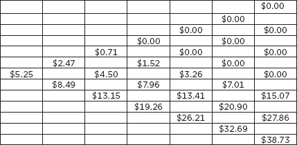
Figure 12.19 shows the use of terminal values to calculate the value of a European put. Figure 12.20 depicts the tree used to value the European put, and Figure 12.21 shows working through a tree European put. By comparison, Figure 12.22 depicts an American put valuation.

FIGURE 12.19

Using Terminal Values to Value European Put

FIGURE 12.20

Tree to Value European Put

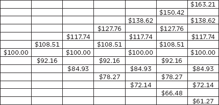
FIGURE 12.21

Working Through Tree European Put

FIGURE 12.22

American Put Valuation

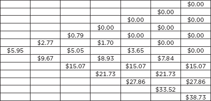
For the European put, the value is the same regardless of whether the terminal values are used or the values are walked back through the tree. Since the European option can’t be exercised early, the value at each node is the discounted weighted average of the next two possible values in the tree. For the American put, the value is the greater of intrinsic value or the discounted weighted average of the next two possible values in the tree. The value of being able to exercise early is equal to the difference in value between the options: ($5.95 − $5.25) = $0.70.

To summarize this model, known as the Cox Ross Rubinstein model:

FORWARD PRICE PRICING MODEL

The forward price pricing model is an alternative model for pricing options that doesn’t rely on the assumption of a lognormal curve distributed around the current price. Instead, it assumes:

• A normal distribution of future prices around the forward price.
• The prices recombine at the forward price at each step.
• The time period and volatility are constants.
• Each step has a 50% up probability and a 50% down probability.

To summarize this model:

FIGURE 12.23

Forward-Centering Binomial Model

Spot = $100

Strike price for call and put = $130

Expiration = 1 year

Steps = 12

Annual volatility = 18%

Risk-free rate = 6%

U = 1.059434237

D = .943900022

P_u = .521709843

P_d = .478290157

TRINOMIAL MODELS

In a trinomial model, it is assumed that the price of the underlying instrument can either go up, go down, or stay flat. In effect, it’s a binomial model that skips every other step. By having this model, you get more nodes and data points at each step along the tree. For example, at the sixth step a binomial model has seven data points whereas a trinomial model has 13 data points.

The other advantage of trinomial models is that by adjusting the time between steps it is possible to set the tree recombination level at a “barrier” level—making it easier to value a barrier option.

Figure 12.24 introduces the Boyle Trinomial Model, and Figure 12.25 shows the Hull White Model.

FIGURE 12.24

Boyle Trinomial Model

FIGURE 12.25

Hull White Model

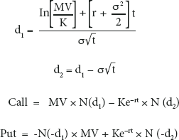
BLACK SCHOLES

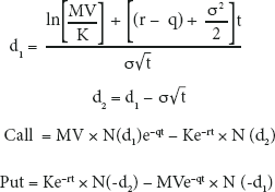
As the time increments between the binomial or trinomial steps become smaller, more data points are available at the terminal value. If the time steps become infinitely small, the solutions for call and put pricing become the integral equation known as Black Scholes (see Figure 12.26). Figures 12.27 through 12.29 depict the use of Black Scholes on underlyings that pay a continuous rate, on futures, and on FX rates, respectively.

FIGURE 12.26

Black Scholes Option Pricing Formula

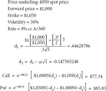
As an example:

Market value = 100

Dividends = $0.00

Strike price = 100

d₁ = .78262

Volatility = 30%

d₂ = .11180

Interest rate = 6%

Call = $37.97

Time frame = 5

Put = $12.05

Notes:

• N stands for the standard normal distribution function—NORM.S.DIST() in Excel.
• For interest calculations, use 360 or actual days—depending on how rate is quoted.
• For trading days, use 250, 252, or 290—depending upon the number of trading days in the market.
• Subtract the PV of any dividends; discount from the ex-date, not payment date.
• Payment of dividends increases short-term volatility—
  reduces long-term volatility.
• Build in expected dividend changes.
• In case of index, convert dividend yield to a continuous rate (q below).

FIGURE 12.27

Black Scholes When Underlying Pays a Continuous Rate

FIGURE 12.28

Pricing Options on Futures

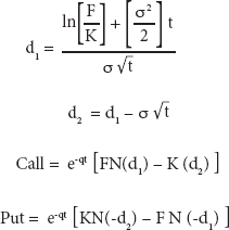
EXAMPLE: OPTION ON PALLADIUM FORWARD

FIGURE 12.29

Options on FX Rates

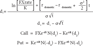
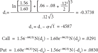
EXAMPLE: CALL ON POUNDS/PUT ON DOLLARS

GBP/USD = $1.56

Strike = $1.60

Dollar rate = 6% cc 30/360

Pound rate = 8% cc 30/360

Volatility = 12%