Principles of Research in Behavioral Science

In Chapter 2, we noted that, from the logical positivist point of view, the experiment is the ideal research strategy. The positivists take this position because, with this research strategy, the experimenter takes complete control of the research situation, determining the independent variable and how it will be manipulated, the dependent variable and how it will be measured, the setting, the participants, and the course of events during the experiment. Experimenters thus create their own artificial universes in which to test their hypotheses. This high degree of control over the research situation allows experimenters to establish the conditions that allow them to determine causality: covariation of proposed cause and effect, time precedence of the cause, and lack of alternatives to the independent variable as explanations for any effects found on the dependent measure. These conditions are reflected in the three defining characteristics of the experiment:

1.	Manipulation of the independent variable. The experimenter creates the conditions to be studied. For example, in an experiment on the effects of stress, the experimenter creates a high-stress condition and a low-stress condition, and assesses the effects of these conditions on a dependent variable. Manipulation of the independent variable in experimentation stands in contrast to research in which the investigator identifies natural situations that differ in their stress levels, measures the level of stress in each situation, and correlates stress scores with scores on the dependent variable. If the independent variable in a study is measured rather than manipulated, the study is not an experiment.
2.	Holding all other variables in the research situation constant. Participants in the experimental and control conditions undergo experiences that are as similar as possible except for the manipulation of the independent variable. In the hypothetical stress experiment, all participants have exactly the same experiences before and after their exposure to high or low stress. As noted in the previous chapter, deviation from this procedure can open the door to alternative explanations for any effects found.
3.	Ensuring that participants in the experimental and control conditions have equivalent personal characteristics and are equivalent with respect to the dependent variable before they take part in the experiment. This equivalence can be attained by holding the characteristics constant across conditions, randomly assigning participants to conditions, matching experimental and control participants on selected characteristics, or having the same people participate in both the experimental and control conditions. These procedures reduce the likelihood of a selection bias.

This chapter discusses three aspects of experimental research. First, we examine the manipulation of the independent variable, considering the roles of experimental and control conditions and the characteristics of a good manipulation. Then, we discuss controlling extraneous variance in experiments by holding potential sources of variance constant and by using various methods of assigning research participants to conditions of the independent variable. We conclude the chapter with a discussion of experiments that use more than two conditions of the independent variable and those that use more than one independent variable. However, before getting into these issues, we must take a brief side trip into the realm of statistics.

A Note on Statistics

Statistics and research design are closely related: Proper research design allows us to collect valid data, and statistics help us to interpret those data. Descriptive statistics, such as the difference between the mean scores of an experimental group and a control group on a dependent variable and the standard deviations of those means, let us know how much effect our independent variable had. Inferential statistics or statistical tests, such as the t-test, analysis of variance (ANOVA), and chi-square tell us how likely it is that the observed effect is real rather than being due to chance differences between the groups. Many of the statistical tests most commonly used in experimental research, such as the t-test and ANOVA, are called parametric statistics and operate by dividing (or partitioning) the variance in the dependent variable scores into two pieces: variance caused by the independent variable and variance caused by everything else in the research situation. Because this concept of partitioning of variance will be important in the discussion of experiments, let’s look at it more closely.

Consider experiments on the effects of stress, in which a common dependent variable is the number of mistakes participants make on a task, such as proofreading a document. Looking at all the participants in the research, both experimental and control, the number of mistakes they make will vary: Some people will make many mistakes, some will make a few, and some will make a moderate number. If stress does affect performance, some of this variance in mistakes made will be due to the independent variable: Some people in the high-stress condition will make more mistakes than people in the low-stress condition. This variance in the dependent variable that results from the independent variable is called treatment (or explained) variance. However, not all the variance in the number of mistakes will be due to the independent variable. Some variance will be due to differences among participants: Some people will be more skilled at the task and so will make fewer mistakes than low-skill people regardless of whether they experience high or low stress. Some people will be more vulnerable to stress and so will make more mistakes in the high-stress condition than their counterparts in the low-stress condition. Variance in the dependent variable can also result from random measurement error (as noted in Chapter 6) and slight unintentional variations in how the experimenter treats each participant. For example, an experimenter who is having a “bad day” might be less patient with that day’s research participants, perhaps speaking abruptly and appearing to be irritated, thereby making that day’s participants more nervous than the participants with whom the experimenter interacts on “good days.” This increased nervousness could cause the participants to make more errors.

From a statistical point of view, all variance in the dependent variable that is not caused by the independent variable is error variance, also called unexplained variance. The value of a parametric statistical test, such as the F value in ANOVA, represents the ratio of treatment variance to error variance—that is, treatment variance divided by error variance. Consequently, the value of a statistical test increases as the treatment variance increases and as the error variance decreases. The larger the value, the less likely it is that the results of the experiment were due to chance factors (the errors represented by the error variance) and the more likely it is that they were due to the effect of the independent variable; in other words, the results are more likely to be “statistically significant.” Therefore, two goals of research design are to increase the effect of the independent variable (and so increase the treatment variance) and to reduce the error variance (and so increase the ratio of treatment to error variance).

Manipulating the Independent Variable

The experimenter manipulates the independent variable to establish conditions that will test the research hypothesis. In its simplest form, the experiment has two conditions, an experimental condition and a control or comparison condition; more complex experiments have additional control or comparison conditions. This section examines the functions of the conditions of an experiment, discusses the characteristics of a good manipulation, and considers situations in which you might want to use multiple stimuli in each condition of the independent variable.

Conditions of the Independent Variable

Experiments can take two forms. Sometimes experimenters want to examine how people behave in the presence of treatment versus its absence; in such situations, the experiment consists of an experimental condition and a control condition. In other cases, experimenters want to compare the effects of two treatments, such as two methods of studying; in such situations, the experiment has two comparison conditions rather than experimental and control conditions.

Experimental and control conditions. In the experimental condition of an experiment, the research participants undergo an experience or treatment that the researcher thinks will affect their behavior. For example, you might hypothesize that knowing the topic of an ambiguous paragraph helps people remember the information presented in it (as did Bransford & Johnson, 1972). In the experimental condition of a study testing this hypothesis, you could tell participants the topic of the paragraph, read the paragraph to them, and then measure their recall of the content of the paragraph. The control condition of the experiment establishes a baseline against which you can assess the effect of the treatment. This baseline consists of an experience that is as similar as possible to that of the experimental condition, except that the treatment is absent. In the example, you would read the paragraph to the research participants and measure their recall without telling them the topic of the paragraph.

This equivalence in experience between the experimental and control conditions lets you rule out what Kazdin (2003) calls nonspecific treatment effects as the cause of any differences between the conditions. Nonspecific treatment effects are changes brought about in participants by all their experiences in the research that do not include the treatment, such as contact with the experimenter, being given a rationale for the research, and so forth. Nonspecific treatment effects are similar to placebo effects, in which people taking part in drug or psychotherapy research improve because they think they are receiving a treatment even if they are being given an inert substance or are not actually undergoing therapy. For example, let’s say you wanted to determine if exercise improves psychological well-being. You obtain a sample of mildly depressed individuals, measure their levels of depression, and assign half to an exercise group and half to a control group. The people in the treatment condition meet for 1 hour 3 days a week for 6 weeks, taking part in an exercise program that you direct. You tell the people in the control condition that you will contact them again in 6 weeks. You assess the participants’ levels of depression at the end of the 6-week period. Under these conditions, it would be impossible to tell if any differences found between the experimental and control groups were due to the effects of the independent variable or to differences in the way in which the two sets of participants were treated. For example, if the people in the experimental condition improved relative to those in the control condition, was the improvement due to the exercise, to their meeting and interacting with each other 3 days a week, or to the attention you gave them? The only way to rule out these alternative explanations would be to have the control participants meet in your presence on the same schedule as the experimental participants, but to perform a task other than exercising, such as a crafts project.

Comparison conditions. Not all experiments include conditions in which the participants experience an absence of or substitute for the experimental treatment. Instead, an experiment might compare the effects of two treatments. For example, you might want to compare the relative efficacy of two ways of studying for a test, such as cramming versus long-term study. Other experiments compare responses to high versus low levels of a treatment. For example, a study of the effect of stress on memory could have a high-stress condition and a low-stress condition. It would be impossible to create a no-stress condition because the requirement for research participants to try to learn and remember material would create some degree of stress even in the absence of an experimental stressor.

Because all experiments compare the effects of different conditions of the independent variable on the dependent variable, some people prefer the term comparison condition to describe what we have called the control condition. Although the term comparison condition is perhaps more descriptive of the true nature of experimental research, we’ve retained the term control condition because it has been used for so long.

Additional Control and Comparison Conditions

Although the archetypical experiment has only two conditions, experimental and control, some experiments have more than one control condition. Two situations that call for multiple control or comparison conditions are when they are required for a complete test of the hypotheses under study and to control for specific alternative explanations for the effect of the independent variable.

Hypothesis testing. Sometimes the hypothesis one is testing has more than one component to it. A complete test of the hypothesis would require the presence of control conditions that would let one test all the components of the hypothesis. Consider an experiment conducted by Bransford and Johnson (1972). They hypothesized that people understand an ambiguous message better and remember its contents better if they have a context in which to put the information, and that comprehension and recall are improved only when people are given the context before they receive the information. Here is one of the paragraphs they used as a message:

The procedure is actually quite simple. First you arrange things into different groups depending on their makeup. Of course, one pile may be sufficient depending on how much there is to do. If you have to go somewhere else due to lack of facilities that is the next step, otherwise you are pretty well set. It is important not to overdo any particular endeavor. That is, it is better to do too few things at once than too many. In the short run this may not seem important, but complications from doing too many can easily arise. A mistake can be expensive as well. The manipulation of the appropriate mechanisms should be self-explanatory, and we need not dwell on it here. At first, the whole procedure will seem complicated. Soon, however, it will become just another facet of life. It is difficult to foresee any end to the necessity for this task in the immediate future, but then one never can tell. (p. 722)

Bransford and Johnson’s (1972) hypothesis had two parts: first, that context improves understanding of and memory for information, and second, for the context to be effective in improving understanding and memory, it must come before the information. Their experiment therefore required three groups of participants: one that received the context before the information, one that received the context after the information, and one that received no context. They tested the first part of their hypothesis by comparing the understanding and recall of the context-before group with those of the no-context group, and they tested the second part of their hypothesis by comparing the context-before group to the context-after group. Their hypothesis would be completely confirmed only if the context-before group performed better than both of the other groups. By the way, the paragraph was about washing clothes, and people who were told the context before hearing the paragraph did understand it and remember its contents better than the people in the other conditions.

Ruling out specific alternative explanations. The baseline control condition allows researchers to rule out nonspecific treatment effects as alternatives to the effect of the independent variable as a cause of experimental and control group differences on the independent variable. Sometimes, however, there are also specific alternative explanations that the experimenter must be able to rule out. In such cases, the experimenter adds control conditions to determine the validity of these alternative explanations. For example, DeLoache and her colleagues (2010) were interested in whether popular DVDs marketed to improve babies’ vocabularies were effective. They used two video conditions: video with no interaction (the parent was in the room while the video played but did not interact with the child) and video with interaction (the parent and child interacted while the video played). A third condition allowed them to test whether parental teaching without a video improved vocabulary. The control condition (no video and no teaching) provided a baseline of normal vocabulary growth. Results showed that babies in the parental teaching condition (without video) gained more vocabulary than babies in the other three conditions. The alternative hypothesis that videos are effective if the parents also interact with the baby was ruled out because vocabulary growth in that condition did not differ from the vocabulary growth in the baseline condition.

Researchers can also use additional control conditions to untangle the effects of natural confounds. Let’s say you conducted an experiment to see if having music playing while studying leads to less learning than not having music playing. If you found that people who studied with music playing learned less than those who studied in silence, you could not definitely attribute the effect to music; after all, any background noise could have detracted from learning. You would therefore need an additional control group who studied to random background noise. Comparing the music condition to the noise condition would tell you if it was music per se that detracted from learning or if it was merely sound that had the effect. Determining the appropriate control or comparison conditions to use is an important aspect of experimental design. Thoroughly analyze your hypothesis to ensure that you test it completely and carefully examine your research design to ensure that you have accounted for all alternative explanations.

Characteristics of a Good Manipulation

In Chapter 6, we saw that two characteristics of a good measure are construct validity and reliability. The procedures used to manipulate an independent variable should also be characterized by construct validity and reliability. In addition, a manipulation must be strong and be salient to participants.

Construct validity. Whenever a manipulation is intended to operationally define a hypothetical construct, one must be sure that the manipulation accurately represents the construct. For example, if you have research participants write essays to manipulate their moods, how do you know their moods actually changed in the ways you wanted them to change? Just as you want to ensure the construct validity of your measures, you also want to ensure the construct validity of your manipulations. The construct validity of a manipulation is tested by means of a manipulation check. The manipulation check tests the convergent validity of the manipulation by checking it against measures of the construct and by ensuring that participants in different conditions of the experiment are experiencing different levels of the independent variable. For example, participants in a high-stress condition should report more stress symptoms than participants in a low-stress condition. A manipulation check should also test the discriminant validity of the manipulation by ensuring that it manipulates only the construct it is supposed to manipulate.

Manipulation checks can take two forms that can be used either separately or together. One way to conduct a manipulation check is to interview research participants after data have been collected, asking them questions that determine if the manipulation had the intended effect. For example, if you were trying to manipulate the degree to which participants perceived a confederate as friendly or unfriendly, as part of your post-experimental interview with participants you could ask them about their perceptions of the confederate. If the manipulation was successful, participants should describe the confederate in ways that are consistent with the manipulation. Post-experimental interview responses can also tell you whether the manipulation was too transparent and that participants might be responding based on experimental demand (see Chapter 7). The other way to conduct a manipulation check is to include dependent variables that assess the construct being manipulated. For example, Schwarz and Clore (1983) assessed the effectiveness of their mood manipulation by having participants complete a mood measure. Statistical analysis of participants’ mood scores showed that participants in the sad-mood condition reported moods that were more negative than those of participants in a neutral-mood condition and that participants in the happy-mood condition reported moods that were more positive than those of the participants in the neutral condition, indicating that the manipulation worked as intended.

Manipulation checks can be made at two points in the research project. The first point is during pilot testing, when the bugs are being worked out of the research procedures. One potential bug is the effectiveness of the manipulation. It is not unusual to have to tinker with the manipulation to ensure that it has the intended effect and only the intended effect. Manipulation checks can also be made during data collection to ensure that all participants experience the independent variable as intended. This is particularly useful if analyses show that the independent variable did not have the expected effect on responses to the dependent variable; results of a manipulation check can suggest reasons for this lack of effect and, in some cases, these possible responses can be incorporated into the data analysis (Wilson, Aronson, & Carlsmith, 2010). Note, however, that if the manipulation check is conducted only concurrently with data collection, it is too late to fix the manipulation if problems are discovered unless you are willing to stop data collection and start the research all over again. Hence, manipulation checks should be used both during pilot testing and in the data collection stage of an experiment. Researchers are sometimes tempted to omit manipulation checks because someone else has used a manipulation successfully. However, it is always wise to include a manipulation check because the validity of manipulations, like that of measures, can vary from one participant population to another.

In the best case, manipulation checks support the validity of the manipulation. But what does the check mean if it fails—that is, if it does not support the manipulation? It is, of course, possible that the manipulation is not valid as an operational definition of the construct. There are, however, other possibilities to consider before abandoning the manipulation. One possibility is that the manipulation is valid but is not strong enough to have the desired impact; we will discuss manipulation strength shortly. Another possibility is that the research participants didn’t notice the manipulation in the context of everything that was happening; we also discuss this issue of salience later. A third possibility is that the measure being used to assess the construct in the manipulation check is not valid or is not sensitive to the effect of the manipulation. Relatedly, the manipulation may have had the desired effect, but participants were not able to state explicitly what they experienced or understood. It is therefore wise to use multiple measures in manipulation checks as well as multiple measures of the dependent variable in the research.

Finally, it is possible the participants are not paying attention to the manipulation. Sometimes participants are inattentive because they are bored or otherwise unmotivated. In other cases, some aspect of the research environment might distract participants from the manipulation. Participants may also adopt the strategy of minimizing their cognitive effort, resulting in satisficing, or responding by choosing the first, rather than the best, response (Krosnick, 1991). Researchers can use an instructional manipulation check (ICM) to assess whether participants have carefully attended to the experimental instructions. To do so, a statement such as this one from a computer-based study is embedded in the instructions:

We are interested in whether you actually take the time to read the directions; if not, then some of our manipulations that rely on changes in the instructions will be ineffective. So, in order to demonstrate that you have read the instructions, please ignore the [items below]. Instead, simply click on the title at the top of this screen. (Oppenheimer, Meyvis, & Davidenko, 2009, Figure 1, p. 868)

For paper and pencil studies, participants can be asked to write “I read the instructions” somewhere on the questionnaire. Oppenheimer et al. (2009) found that the participants who failed to follow IMC instructions spent significantly less time on the study and were lower in the need for cognition than participants who followed the IMC instructions; dropping these participants can reduce error variance and increase the researchers’ ability to detect a difference between experimental conditions.

Reliability. In Chapter 6, we noted that a reliable measure is a consistent measure, one that gives essentially the same results every time it is used. Similarly, reliability of manipulation consists of consistency of manipulation: Every time a manipulation is applied, it is applied in the same way. If a manipulation is applied reliably, every participant in the experiment experiences it in essentially the same way. High reliability can be attained by automating the experiment, but as pointed out in the Chapter 7, automation has severe drawbacks (see also Wilson et al., 2010). High reliability can also be attained by preparing detailed scripts for experimenters to follow and by rehearsing experimenters until they can conduct every condition of the experiment correctly and consistently. Remember that low reliability leads to low validity; no matter how valid a manipulation is in principle, if it is not applied reliably, it is useless.

Strength. A strong manipulation is one in which the conditions of the independent variable are different enough to differentially affect behavior. Let’s say, for example, that you’re interested in the effects of lighting level on work performance. You hypothesize that brighter light improves performance on an assembly task; the dependent variables will be speed of assembly and the number of errors made. You test the hypothesis by having half the participants in your experiment work under a 60-watt light and the others under a 75-watt light. It would not be surprising to find no difference in performance between the groups: The difference in lighting level is not large enough to have an effect on performance.

Strong manipulations are achieved by using extreme levels of the independent variable. The lighting and work performance study, for example, might use 15-watt and 100-watt lights to have more impact on behavior and so increase the amount of treatment variance in the dependent variable. Although it is desirable to have a strong manipulation, there are two factors to consider in choosing the strength of a manipulation. One consideration is realism: An overly extreme manipulation might be unrealistic. For example, it would be unrealistic to use total darkness and 1,000-watt light as the conditions in the lighting experiment: People almost never do assembly tasks under those conditions. A lack of realism has two disadvantages. First, participants might not take the research seriously and so provide data of unknown validity. Second, even if there were no internal validity problems, it is unlikely that the results would generalize to any real-life situations to which the research was intended to apply. Smith (2000) recommends using manipulations that match situations found in everyday life. For example, a study of responses to accident scenarios with mild and severe consequences can be based on media accounts of such events. The second consideration is ethical: An extreme manipulation might unduly harm research participants. There are, for example, ethical limits on the amount of stress to which a researcher can subject participants; for example, experimental research cannot ethically examine responses to naturally occurring events, such as the death of a close relative or someone witnessing a murder (Smith, 2000)

There is an exception to the general rule that stronger manipulations are better for obtaining differences between conditions on the dependent variable. As we will discuss shortly, sometimes the relationship between the independent and dependent variables is U-shaped. Under such conditions, the largest differences in behavior will show up not when the two extreme conditions are compared but, rather, when the extremes are compared to a moderate level of the independent variable.

Salience. For a manipulation to affect research participants, they have to notice it in the context of everything else that is happening in the experiment. This characteristic of “noticeability” is called salience. A salient manipulation stands out from the background, and it is sometimes necessary to put a lot of effort into establishing the salience of a manipulation. For example, Landy and Aronson (1968) conducted a study to determine whether people react more strongly to evaluations of them made by another person if they think that person is especially discerning, that is, especially skilled in deducing the personality characteristics of other people. The researchers manipulated how discerning the other person appeared by having him perform a task, in the presence of the participant, designed to show either the presence (experimental condition) or absence (control condition) of discernment. But how could the researchers be sure the participants noticed how discerning the other person was? They

told the subject that “degree of discernment” was an aspect of the confederate’s behavior that was of particular interest to them; asked the subject to rate the confederate’s discernment; [and] informed the subject exactly how the confederate’s behavior might reflect either high or low discernment. (Aronson, Ellsworth, Carlsmith, & Gonzales, 1990, pp. 223–224)

Not all manipulations require this degree of emphasis, but experimenters do need to ensure that the participants notice the manipulation. When experimental instructions involving the manipulation are complex, researchers should present the information in different ways to ensure comprehension (Wilson et al., 2010); for example, providing both verbal and written information may be necessary to ensure that a manipulation is noticed.

Using Multiple Stimuli

The stimulus is the person, object, or event that represents the operational definition of a condition of the independent variable and to which research participants respond. For example, in a study on whether physical attractiveness affects person perception, the independent variable is physical attractiveness and its operational definition might be pictures of a person made up to appear attractive or unattractive. A stimulus would be the particular picture to which a research participant responds with an evaluation. When the independent variable is a manifest variable, only one stimulus can represent one of its conditions. For example, in a study of the effects of caffeine on physiological arousal, a condition in which participants ingest 100 mg of caffeine can be represented only by a stimulus that consists of 100 mg of caffeine. However, when the independent variable is a hypothetical construct, it can very often be represented by any number of stimuli. In the physical attractiveness study, for example, the concept of physical attractiveness could be represented by pictures of any of thousands of people or by computer-generated stimuli that were manipulated to represent attractive or unattractive faces. For example, Langlois and Roggman (1990) hypothesized that “average” faces are seen as more attractive than unique faces. To test this, they created a set of average faces by digitizing a set of photographs and using them to create composite photos that participants then evaluated.

Although many constructs can be represented by multiple stimuli, most research dealing with such constructs uses only one stimulus to represent any one condition of the independent variable, such as one picture of an attractive person and one picture of an unattractive person. If the research finds a difference between the conditions, a problem arises in interpreting the results: Although the outcome could be due to the effects of the independent variable, it could also be due to the unique features of the stimulus or to an interaction between the independent variable and the unique features of the stimulus (Wells & Windschitl, 1999). Let’s say, for example, that the stimuli used in our hypothetical attractiveness study were pictures of a model made up to portray an attractive person in one picture and an unattractive person in the other picture. In making their evaluations, were the participants responding to the general construct of physical attractiveness—the intended independent variable—or to the unique characteristics of the particular model who posed for the pictures, such as the shape of her face, the size of her mouth, and the distance between her eyes? That is, were the research participants responding to the general characteristic of physical attractiveness or to the unique characteristics of that particular person? There is no way to answer this question if only a single, unique stimulus is used to represent each condition of the independent variable.

The question would have an answer, however, if each research participant had responded to a set of stimuli consisting of a sample of the possible stimuli that could represent the conditions of the independent variable. For example, you could have participants in each condition of the experiment rate four people rather than just one. With multiple stimuli per condition, it becomes possible to apply a special form of ANOVA, called the random effects model, that separates the variance in the dependent variable due to specific stimuli, such as the models used to portray the attractive people, from the variance due to the hypothesized construct represented by the stimuli, such as the concept of “attractive person.” This form of ANOVA is extremely complex (Richter & Seay, 1987), but because it separates irrelevant stimulus variance from the relevant variance due to the hypothetical construct, it provides a much more valid test of the effects of the independent variable than would the use of a single stimulus per condition. If an independent variable is treated as a random factor, the researcher can be more confident that the experimental results generalize to other, similar methods of manipulating the variable of interest (Smith, 2000).

Controlling Extraneous Variance

The experiment is characterized not only by manipulation of the independent variable but also by procedures used to control factors that cause extraneous variance in the dependent variable. As noted earlier, any variance in the dependent variable that is not caused by the independent variable is considered error variance. Some of this variance is due to random factors, such as slight variations in the way the experimenter treats research participants. Other variance is due to factors that are systematically related to the dependent variable but are not of interest to the researcher. For example, there are cultural differences on many variables that behavioral scientists study (Matsumoto & Juang, 2013), but these differences are not of interest to all researchers. Variables that are related to or can influence the dependent variable in a study but are not a focus of the research are called extraneous variables. When extraneous variables are not treated as independent variables in the research, their effects form part of the error variance in the statistical analysis of the data. Experimenters therefore take steps to control extraneous variance.

Holding Extraneous Variables Constant

Extraneous variables that are part of the research situation, such as the characteristic of the room in which the research takes place, are fairly easy to control: The experimenter holds these variables constant across conditions of the independent variable. Because these factors do not vary as part of the experiment, they cannot cause systematic variance in the dependent variable—their effects are reasonably constant for each participant in the research. Individual differences in participants’ responses to these controlled variables form part of the error variance in the experiment.

Extraneous variables that are characteristics of the research participants, such as personality and background, are more difficult to control: Differences among people, unlike differences among rooms, cannot always be eliminated by the actions of the experimenter. Nevertheless, it is sometimes possible to hold participant variables constant. For example, Weis and Cerankosky (2010) included only boys in their study of how video-game usage affected academic achievement because previous research had demonstrated gender differences in video game choice and frequency of play and the researchers wanted to control for these effects. However, as pointed out in Chapter 5, this strategy can bias the results of research and limit their generalizability if participants with only one characteristic of the extraneous variable—for example, only boys—are used in all research on a topic. As discussed in more detail later, you can avoid this problem by treating participant characteristics as independent variables in experiments. Researchers must balance the costs and benefits of doing so; for example, Weis and Cerankosky (2010) provided video consoles and games to their participants, so including girls (and thus doubling their sample size) would have significantly increased their expenses and the time required to complete the study with perhaps little predictive gain in their obtained results.

Experimenters most commonly control the effects of variance in research participants’ personal characteristics by the ways in which they assign participants to conditions of the independent variable. In between-subjects designs (also called independent groups designs), a participant takes part in either the experimental or control condition, but not both. The researcher distributes the effects of extraneous participant variables evenly across the experimental and control groups by either randomly assigning participants to conditions or matching the participants in each condition on key extraneous variables. In within-subjects designs (also called repeated measures designs), each participant takes part in both the experimental and control conditions so that the effects of participant variables are perfectly balanced across conditions.

Between-Subjects Designs

Between-subjects designs are more commonly used in behavioral research than are within-subjects designs. Some reasons for this preference will be discussed later in comparing the advantages and disadvantages of these types of designs. Because between-subjects designs have different people in the experimental and control groups, a major consideration in using them is ensuring that participants in the two groups are equivalent in their personal characteristics. Experimenters can use two strategies to attain equivalence: simple random assignment of participants to conditions and matched random assignment.

Simple random assignment. The strategy most often used to assign participants to groups is simple random assignment. When a participant arrives to take part in the experiment, the experimenter uses a random procedure, such as a table of random numbers or flipping a coin, to determine if the participant will be in the experimental or control condition. For example, an even number or “heads” could mean the control condition, and an odd number or “tails” the experimental condition. When you use random assignment, you assume that, because group assignments are random, members of the two groups will, on the average, have the same personal characteristics. For example, if some participants are unusually skilled at the research task and others unusually unskilled, then randomly assigning people to groups should put about half the skilled and half the unskilled people in each group. Consequently, the effects of their skill should cancel out when the groups’ mean scores on the task are compared.

Consider an experiment that tests the effects of practice on memory (Kidd & Greenwald, 1988). Participants listen as the experimenter reads a 9-digit number to them; they then must correctly recall it. They do this 96 times. Participants in the experimental condition are given four task-relevant practice sessions before being tested “for the record,” whereas the participants in the control condition practice a different memory task. Without practice on the actual task, participants can correctly recall an average of 60% of the numbers. Let’s assume that an unusually skilled person can correctly recall 70% of the numbers without practice and that an unusually unskilled person can recall 50%. Let’s say you do an experiment such as this with six participants: two who happen to be highly skilled, two with average skill, and two with unusually low skill. Simple random assignment puts one person from each skill level into each condition of the experiment. The first column in Table 9.1 shows the effect of random assignment: The average skill level of each group is the same. Let’s say that, as Kidd and Greenwald found, four task-relevant practice sessions added 20 percentage points to a person’s score and that irrelevant practice neither helps nor hinders memory. The second column in Table 9.1 shows the effect of practice, and the third column shows the participants’ total scores (skill plus practice effects). Because the different skill levels are equally distributed between the two experimental conditions, the difference in the groups’ mean total scores is the same as the effect of the independent variable: 20 percentage points. Random assignment therefore controls the effects of participant characteristics by balancing them out across groups. In research in which the independent variable is manipulated using material in a questionnaire, participants can also be randomly assigned to conditions by randomizing the experimental and control versions of the questionnaire before distributing them.

As an alternative to true random assignment, researchers sometimes use what might be called “quasi-random” assignment. Under this procedure, the researcher assigns participants alternately to the experimental and control conditions as they come to the laboratory: The first person to arrive goes into the experimental condition, the second to the control condition, the third to the experimental condition, and so forth. This procedure assumes that the order in which people arrive for the experiment is random so that the even-numbered people are, on the average, equivalent to the odd numbered people. However, the validity of this assumption is open to question: People who are more motivated to participate in the study might arrive earlier, thereby inducing a self-selection bias into the experiment. Therefore, never use such quasi-random procedures.

Random assignment of participants to conditions does not guarantee that the members of the experimental and control group will be equivalent. Although equivalence or near-equivalence will be the most common outcome of randomization (Strube, 1991), there is a real, albeit small, possibility of the groups’ being very different. For example, if you had a participant pool composed of 10 men and 10 women and randomly assigned them to experimental and control groups, there is about a 1 in 2,400 chance of getting a group with 8 or more men in it. These odds are probably good enough for most research, but researchers who want to can exercise more control over the characteristics of the members of the experimental and control group by matching the members of the groups on important personal characteristics.

TABLE 9.1

Effect of Simple Random Assignment

Simple random assignment evenly distributes people with different skill levels among the conditions of an experiment so that individual differences in skill do not affect the difference in the mean scores found in the conditions.

	Nine-Digit Numbers Recalled Correctly
Experimental Condition	Effect of Skill	Practice	Effect of Total Score
Person A	70%	+20%	90%
Person B	60%	+20%	80%
Person C	50%	+20%	70%
Mean	60%	+20%	80%
Control Condition
Person A	70%	0%	70%
Person B	60%	0%	60%
Person C	50%	0%	50%
Mean	60%	0%	60%

Matched random assignment With matched random assignment of participants to conditions, the researcher attempts to ensure that the members of the experimental and control groups are equivalent on one or more characteristics. The researcher does this by first measuring the characteristic and then balancing group membership on the characteristic. For example, in their study of the effect of drug glucose levels on dogs’ self-control, Miller, Pattison, DeWall, Rayburn-Reeves, & Zentall (2010, Study Two) matched dogs on their training histories and on their breed. One member of each pair was then assigned to the self-control condition or to the control condition; this pair was then randomly assigned to either the glucose group or the placebo group.

Matching on participants’ physical characteristics, such as breed of dog, is fairly easy; for other characteristics, such as IQ and personality, it is more difficult. For these kinds of characteristics, you must first pretest all potential participants to determine their scores on the variable. You must then rank order the people by their scores and then divide them into pairs from the top down. The first member of each pair is randomly assigned to either the experimental or control group; the other member of the pair is assigned to the other group. Figure 9.1 illustrates this process for 10 people ranging in IQ score from 125 to 110. The mean IQ scores of the experimental and control groups are 116.8 and 116.0, a trivial difference. Nonrandom assignment, such as putting the odd-numbered people (those ranked first, third, and so on) in the experimental group and the even numbered people in the control group, results in a larger difference in mean IQ scores: 117.4 for the experimental group and 116.0 for the control group. A major drawback of matched random assignment for psychological characteristics is the cost, in time, money, and resources, of pretesting. In addition, as discussed in Chapter 7, pretesting may cause internal validity problems. Matched random assignment is therefore normally used only when the control variable is known to have a strong effect on the dependent variable and the researcher wants more control over it than simple random assignment affords.

FIGURE 9.1

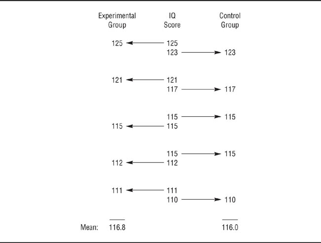
Matched Random Assignment.

The researcher first measures the participants’ scores on the matching variable (in this case IQ), rank orders participants by score, divides them into pairs, and randomly assigns the members of the pairs to the experimental and control conditions.

Within-Subjects Designs

In within-subjects (or repeated measures) designs, each research participant experiences both the experimental and control conditions of the independent variable. Consider, for example, the study of the effect of practice on memory for 9-digit numbers, discussed earlier. In a between-subjects design, each participant would be tested once, either after a task-relevant practice session or after a task-irrelevant practice session. In a within-subjects design, each participant would be tested twice, once after a task-relevant practice session and once after a task-irrelevant practice session. Let’s look at some of the advantages and limitations of within-subjects designs.

Advantages relative to between-subjects designs. Because participants in within-subjects designs take part in both the experimental and control conditions, these designs result in perfect equivalence of participants in both conditions. Because the same people are in each condition, the personal characteristics of the participants match perfectly. This perfect matching results in one of the primary advantages that within-subjects designs have over between-subjects designs: reduced error variance. This reduction in error variance means that within-subjects experiments are more likely than equivalent between-subjects experiments to produce statistically significant results.

This advantage will be stronger to the extent that participant characteristics affect scores on the dependent variable. A second advantage of within-subjects designs is that because the same people participate in both the experimental and control conditions, a two-condition within-subjects design requires only half the number of participants required by the equivalent between-subjects design. This advantage can be especially useful when people are selected for participation in research on the basis of a rarely occurring characteristic, such as an unusual psychiatric disorder.

The problem of order effects. Despite these advantages, researchers use within-subjects designs much less frequently than between-subjects designs. This less frequent use results from a set of disadvantages inherent in within-subjects designs referred to collectively as order effects. An order effect occurs when participants’ scores on the dependent variable are affected by the order in which they experience the conditions of the independent variable. For example, participants might do better on whichever condition they experience second, regardless of whether it is the experimental or control condition. There are four general categories of order effects: practice effects, fatigue effects, carryover effects, and sensitization effects (Greenwald, 1976).

Practice effects are differences on the dependent variable that result from repeatedly performing the experimental task. For example, when people are faced with an unfamiliar task, they often do poorly the first time they try it but improve with practice. The more often the experiment requires them to engage in a task, the better participants become at it. Another kind of practice effect relates to the independent variable. Let’s say you are conducting a study on the effects of stress, using background noise as the stressor. Over time, participants might habituate to, or become used to, the noise so that it has less effect on their performance. Fatigue effects, in contrast, result when participants become tired or bored from repeatedly performing the same task. Unlike practice effects, fatigue effects lead to decrements in performance.

Carryover effects occur when the effect of one condition of the experiment carries over to and affects participants’ performance in another condition. Let’s say you are conducting a study of the effects of caffeine consumption on reaction time. In the experimental condition you give participants a standardized dose of caffeine, and in the control condition you give them an inert substance. If participants take part in the caffeine condition first, the effects of the drug might still be present in their bodies when they take part in the control condition. The effects of the caffeine can then “carry over” and affect performance in the control condition. However, you wouldn’t want to give all participants the inert substance first, because practice effects would then be confounded with the effects of the caffeine in the experimental condition.

Sensitization effects are a form of reactivity: Experiencing one condition of the experiment affects their performance in the other condition. For example, Wexley, Yukl, Kovacs, and Sanders (1972) studied the effect of raters’ exposure to very highly qualified and very poorly qualified job applicants on ratings of average applicants. Participants watched videotapes of three job interviews. In one condition, they saw the interviews of two highly qualified applicants prior to the interview of an average applicant; in another condition, participants saw the interviews of two poorly qualified applicants followed by that of an average applicant. When seen in isolation, the average applicant received a mean rating of 5.5 on a 9-point scale; when seen following the highly qualified applicants, the average applicant’s mean rating was 2.5, whereas following the poorly qualified applicants the mean rating was 8.1.

Sensitization can also induce demand characteristics when exposure to more than one condition of the independent variable allows research participants to form hypotheses about the purpose of the research or calls forth a social desirability response bias (see Chapter 7). Let’s say you’re conducting a study on the effects of physical attractiveness on how likable a person is perceived to be. In one condition, you show participants a picture of a physically attractive person and in the other condition, a picture of a less attractive person. You ask participants to rate the person in the picture on the degree to which they thought they would like the person if they met him or her. Participants will probably respond naturally to the first picture, giving their true estimate of likability, but when they see the second picture, problems could arise. Because it is socially undesirable to evaluate people solely on the basis of appearance, participants might deliberately manipulate their responses giving the same rating to the person in the second picture that they gave to the person in the first picture, even if their true responses are different.

Controlling order effects. In some cases, the researcher can design a within-subjects experiment in ways that control for order effects. Practice effects can be controlled by counterbalancing the order in which participants experience the experimental and control conditions. Half the participants undergo the experimental condition first, and the other half undergo the control condition first. This procedure is designed to spread practice effects evenly across the conditions so that they cancel out when the conditions are compared.

Counterbalancing is easy to carry out when an experiment has only two conditions. For example, the left side of Table 9.2 illustrates counterbalanced orders of conditions for a two-condition (Conditions A and B) experiment. As you see, there are only two orders in which participants can experience the conditions: A before B and B before A. However, as discussed later in this chapter, experiments frequently have three or more conditions; under these circumstances, counterbalancing becomes much more difficult because all possible orderings of conditions must be used: Each condition must appear in each position in the ordering sequence an equal number of times to balance the order in which participants experience the conditions, and each condition must follow every other condition an equal number of times to balance the sequencing of conditions. These rules are met for the three-condition (A, B, and C) experiment illustrated on the right side of Table 9.2. Condition A, for example, appears in each position in the order (first in rows 1 and 2, second in rows 3 and 5, and third in rows 4 and 6) and precedes Condition B twice (in rows 1 and 5) and follows Condition B twice (in rows 3 and 6). Notice that the three-condition experiment requires that participants be divided into six groups in order to completely counterbalance the order of conditions. The number of orders increases dramatically with the number of conditions: Four conditions would require 24 orders of conditions, and five conditions, 120 orders.

TABLE 9.2

Counterbalancing in Two-and Three-Condition Within-Subjects Experiments

Each condition appears in each order of the sequence, and each condition appears before and after every other condition.

Two Conditions		Three Conditions
A	B	A	B	C
B	A	A	C	B
		B	A	C
		B	C	A
		C	A	B
		C	B	A

Because the number of condition orders required by complete counterbalancing can quickly become enormous as the number of conditions increases, partial counterbalancing is frequently used for more than three conditions. One way to partially counterbalance is to randomly assign a different order of conditions to each participant. A more systematic technique is to use a Latin square design (Fisher & Yates, 1963). In this design, the number of orders is equal to the number of conditions, with each condition appearing in each place in the order. The left side of Table 9.3 shows the basic Latin square design for a four-condition experiment. As you can see, each of the conditions comes in each of the possible places in the four orders. For example, Condition A comes first in row 1, fourth in row 2, third in row 3, and second in row 4. The basic Latin square design therefore balances the order of conditions, but not their sequencing. For example, except when it comes first in a row, Condition B always follows Condition A and precedes Condition C. Sequencing can be partially controlled by using a balanced Latin square design: each condition is preceded once by every other condition. For example, in the balanced design on the right side of Table 9.3, Condition B is preceded by Condition A in row 1, by Condition D in row 3, and by Condition C in row 4. Although the balanced Latin square design controls the sequencing of pairs of conditions, it does not control higher order sequences; for example, the sequence ABC precedes, but does not follow, Condition D.

Counterbalancing can also be used to distribute carryover effects across conditions. However, it is better to also insert a washout period between conditions. A washout period is a period of time over which the effects of a condition dissipate. For example, in the hypothetical study of the effects of caffeine on arousal, described earlier, you might have participants undergo one condition one day and have them come back for the other condition the next day without consuming any caffeine in the interim. The purpose of this procedure is to allow the caffeine to “wash out” of the bodies of those participants who experienced the experimental condition first so that it does not affect their performance in the control condition. The washout period might be minutes, hours, or days, depending on how long the effects of a condition can be expected to last.

Sensitization effects are harder to control than practice or carryover effects. Although counterbalancing will spread these effects across conditions, it will not eliminate the effects of any demand characteristics produced. Therefore, it is best not to use a within-subjects design when sensitization effects are likely to produce demand characteristics, as in the physical attractiveness example given earlier.

TABLE 9.3

Basic and Balanced Latin Squares Designs

Order of Conditions

Basic Design

Balanced Design

1

A

B

C

D

1

A

B

C

D

2

B

C

D

A

2

B

D

A

C

3

C

D

A

B

3

C

A

D

B

4

D

A

B

C

4

D

C

B

A

TABLE 9.4

Differential Order Effects

Order of participation in the conditions has a greater effect when the experimental condition is experienced after the control condition.

	Condition
	Experimental (E)	Control (C)	Difference
True performance level	40	30	10
Order effect for E→C	0	10
Order effect for C→E	20	0
Observed Score	60	40	20

The use of counterbalancing assumes that order effects are equal regardless of the sequence in which participants experience the conditions. For example, in a two-condition experiment, counterbalancing assumes that the order effect for participating in the experimental condition (E) first is the same as the order effect for participating in the control condition (C) first. Table 9.4 illustrates this differential order effect. The true effect of the independent variable is to increase participants’ scores on the dependent variable by 10 points in the experimental condition compared to the control condition. Experiencing the experimental condition first adds another 10 points to their scores in the control condition. However, experiencing the control condition first adds 20 points to the scores in the experimental condition. This differential order effect (C before E greater than E before C) artificially increases the observed difference between the conditions by 10 points, resulting in an overestimation of the effect of the independent variable. Order effects can be detected by using a factorial experimental design, discussed later in the chapter.

When order effects are good. Before leaving the topic of order effects, it is important to note that order effects are not always bad; sometimes, researchers want an order effect because it is the variable being studied. For example, an educational researcher might be interested in the effects of practice on learning, a psychopharmacologist might be interested in carryover effects of drugs, or a person studying achievement motivation might be interested in sensitization effects, such as the effect on motivation of success followed by failure compared to the effect of failure followed by success. In none of these cases would it be appropriate to control order effects.

Multiple-Group Designs

Quantitative Independent Variables

When studying the effects of quantitative independent variables, researchers are usually interested in determining the effects on the dependent variable of adding more of the independent variable. These effects can be classified in terms of two general categories of relationships that can exist between an independent variable and a dependent variable. In linear relationships, scores on the dependent variable increase or decrease constantly as the level of the independent variable increases or decreases; the relationship can be graphed as a straight line. Panels (a) and (b) of Figure 9.2 illustrate the two types of linear relations. In a positive relationship, panel (a), scores on the dependent variable increase as the level of the independent variable increases; in a negative relationship, panel (b), scores on the dependent variable decrease as the level of the independent variable increases. In the second category of relationships, curvilinear relationships, the relationship between the independent variable and the dependent variable takes a form other than a straight line. Panel (c) of Figure 9.2 illustrates some curvilinear relationships.

FIGURE 9.2

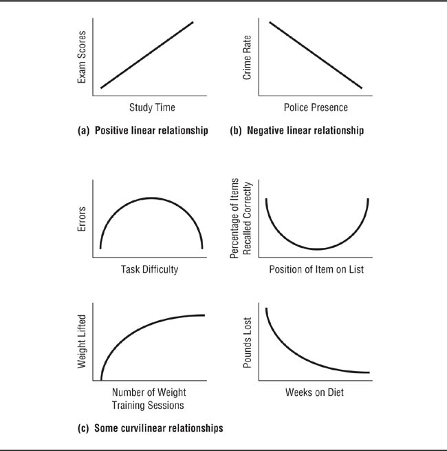
Examples of Linear and Curvilinear Relationships

Many researchers use designs with only two levels of an independent variable, in part because doing so maximizes simplicity and increases statistical power (Smith, 2000). However, there is a very good reason to consider using at least three levels of the variable of interest. Specifically, if there is a curvilinear relationship between the independent variable and the dependent variable, it can be found only if there are more than two levels of the independent variable. Why? If you have only two points on a graph, you can draw only a straight line between the two points, which represents a linear relationship. If you have more than two points, you can draw a curved line if that’s what the points represent. This idea is illustrated by three studies, described in the previous chapter, on the effect of a person’s degree of responsibility for a crime on how much punishment people think is appropriate.

In Chapter 8 we described a series of studies on the relationship between defendant responsibility for a crime and recommended punishment. In the first study we described, the defendant in an armed robbery trial had either a high degree of responsibility for planning and executing the crime (85% responsible) or a lesser degree of responsibility (15% responsible; DeJong, Morris, & Hastork, 1976). Results showed that people who were in the high responsibility condition recommended longer sentences than people who had read the less-responsibility summary. However, results of a replication study, in which the high degree of responsibility was defined as 85% responsible, but the low degree responsibility was operationally defined as 50% responsible, showed no relationship between degree of responsibility for the crime and the punishment assigned by research participants: Both criminals were assigned sentences of about the same length (Feldman & Rosen, 1978). Panels (a) and (b) of Figure 9.3 illustrate the results of these studies. Whitley’s (1982) replication employed a three-group design in which the defendant had 15%, or 50%, or 85% responsibility for the crime. The results of this study, illustrated in panel (c) of Figure 9.3, showed a curvilinear relationship between responsibility and punishment: punishment rose as responsibility increased up to 50% and then leveled off. These results replicated those of both DeJong et al. (1976) and Feldman and Rosen (1978).

FIGURE 9.3

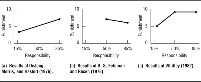
Using Three Levels of a Quantitative Independent Variable.

Only when all three levels are used does the true curvilinear relationship between the variables become apparent.

As these studies show, it is extremely important to look for curvilinear effects when studying quantitative independent variables. It would be appropriate to use just two groups only if there is a substantial body of research using multiple-group designs that showed that only a linear relationship existed between the independent and dependent variables that you are studying. However, when using multiple levels of an independent variable you should ensure that the levels represent the entire range of the variable. For example, DeJong et al. (1976) could have used three levels of responsibility—say, 15%, 33%, and 50%—and still not have detected the curvilinear relationship because the curve begins beyond that range of values. Similarly, Feldman and Rosen (1978) would still have concluded that no relationship existed if they had used 50%, 67%, and 85% as their levels of responsibility.

Qualitative Independent Variables

Multiple-group designs that use qualitative independent variables compare conditions that differ in characteristics rather than amount. For example, a researcher might be interested in how research participants react to people who are depressed compared to people who are schizophrenic and to people having no psychiatric diagnosis. Qualitative independent variables are also involved when a study requires more than one control group. For example, the Bransford and Johnson (1972) study, described earlier, had one experimental group—participants who were given the context before the information—and two control groups—no context and context after the information. One can also have one control group and more than one experimental group. Kremer and Stephens (1983), for example, wanted to see whether information about the state of mind of a rude person affected how victims of the rudeness evaluated the person and how the timing of the information affected evaluations. Research participants were annoyed by a confederate of the researchers who was acting as an experimenter for the study. They were then put into one of three conditions. In one experimental condition, another person posing as a colleague of the experimenter told the participants immediately after they had been rudely treated that the confederate had been having a bad day and did not usually act like that. Participants in the second experimental condition received the same information, but only after a delay of several minutes. Participants in the baseline condition received no information about the experimenter’s state of mind. All participants were given an opportunity to evaluate the experimenter by recommending, using a 7-point scale, whether he should continue to receive research funding, with a rating of 1 meaning “Give the funds to someone else” and a rating of 7 meaning “Give the funds to the experimenter.” The results of the study are illustrated in Figure 9.4: Information about the confederate’s state of mind led to more positive evaluations, but only if the participants received the information immediately after being annoyed.

FIGURE 9.4

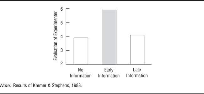
Two Experimental Conditions Compare the Timing of Information to a No-Information Control Condition.

The difference between the early and late information conditions shows the importance of the timing of presentation of the information. Post hoc tests indicate the group represented by a shaded bar is significantly different from the other two groups.

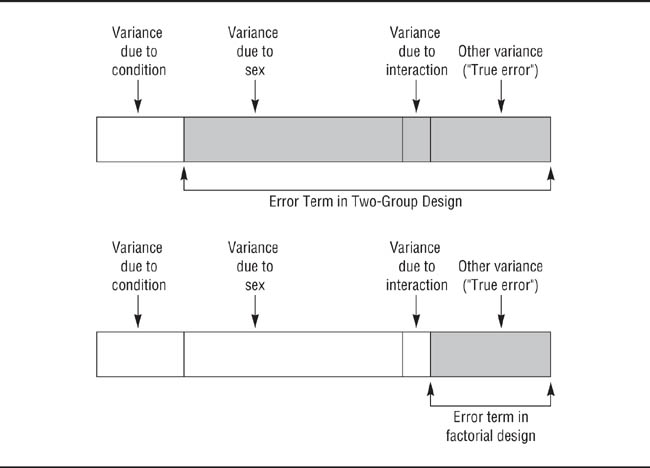
Interpreting the Results of Multiple-Group Experiments

Multiple-group designs are very useful to the research psychologist, potentially providing a wealth of information unavailable from two-group designs and providing additional controls for threats to the internal validity of the research. However, a potential pitfall exists in the interpretation of the results of the statistical analysis of these designs. The data from multiple-group designs are analyzed using what is known as a one-way analysis of variance (ANOVA), which was designed for this purpose. The statistical test in ANOVA is the F test, which is analogous to the t-test in two-group designs. A statistically significant F value means that out of all the possible two-group comparisons among the group means, at least one comparison is statistically significant; however, it does not tell you which comparison is significant. For example, Kremer and Stephens’s (1983) data analysis found a significant F value, but it did not tell them which of the three comparisons among group means was significant (Figure 9.4): no information versus early information, no information versus late information, or early information versus late information.

To determine the significant difference or differences, you must conduct a post hoc (or after-the-fact) analysis, which directly compares the group means. When you have specific hypotheses about differences in means, the comparisons among those means are made with a priori (or preplanned) contrasts. Similar comparisons must be made when a quantitative independent variable is used to determine where the significant differences among groups lie. There are also specific a priori contrasts that help you determine if the effect found is linear or curvilinear. Kremer and Stephens’s (1983) a priori contrast analysis found that the differences between the means of the early-information and no-information groups and between the early-information and late-information groups were significant, but that the difference between the no-information and late-information groups was not. These results showed that both the information and the timing of the information affected evaluations of the confederate.

Never interpret the results of a multiple-group experiment solely on the basis of the F test; the appropriate post hoc or a priori analyses should always be conducted. Most statistics textbooks describe how to conduct these analyses.

Factorial Designs

Up to this point, the discussion of research has assumed that any one study uses only one independent variable. However, much, if not most, research in behavioral science uses two or more independent variables. Designs with multiple independent variables are called factorial designs; each independent variable is a factor in the design. This section looks at the nature of factorial designs, discusses the interpretation of interaction effects, considers some of the uses of factorial designs, and examines some of the forms that factorial designs can take.

The Nature of Factorial Designs

Factorial designs can be very complex, so this section introduces the topic by discussing the shorthand that researchers use to describe factorial designs, the kinds of information that factorial designs provide, and the various outcomes that can result when factorial designs are used.

Describing factorial designs. By convention, a factorial design is described in terms of the number of independent variables it uses and the number of conditions or levels of each independent variable. A 2 × 2 (read as “2 by 2”) design, for example, has two independent variables, each with two conditions. The number of numbers (in this case the two 2s) indicates the number of independent variables; the numbers themselves indicate the number of conditions of each independent variable. A 3 × 2 design has two independent variables, one with three conditions (indicated by the 3) and the other with two conditions (indicated by the 2); a 3 × 2 × 2 design has three independent variables, one with three conditions and the others with two conditions each. For the sake of simplicity, most of this discussion of factorial designs deals only with 2 × 2 designs. Bear in mind, however, that the same principles apply to all factorial designs regardless of complexity.

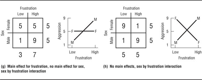
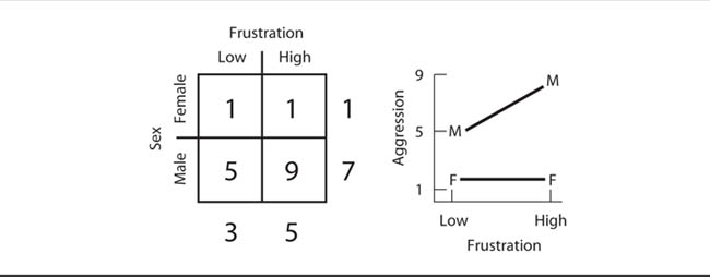
Information provided by factorial designs. Factorial designs provide two types of information about the effects of the independent variables. A main effect is the effect that one independent variable has independently of the effect of the other independent variable. The main effect of an independent variable represents what you would have found if you conducted the experiment using only that independent variable and ignored the possible effects of the other independent variable. For example, if you studied the effects of frustration on aggression in men and women, the main effect for frustration is the difference in mean aggression scores between the frustrated group and the nonfrustrated group ignoring the fact that both groups were composed of both men and women. An interaction effect (or simply “interaction”) occurs when two or more independent variables combine to produce an effect over and above their main effects. Interactions can be seen only when the effects of two or more independent variables are considered simultaneously; consequently, interaction effects can be found only when a factorial design is used.

Let’s look at a study conducted by Platz and Hosch (1988) as an example of a factorial design. Platz and Hosch were interested in the accuracy of cross-racial identifications, specifically in whether people are able to identify members of their own races more accurately than members of other races. Although Platz and Hosch used a 3 × 3 design, for now let’s consider only two conditions of each of the independent variables. They had Black confederates and White confederates buy something in a convenience store staffed by Black clerks or White clerks. Two hours later, the clerks were asked to pick the customers out from sets of facial photographs. The researchers found that identification accuracy depended on both the race of the clerk and the race of the customer; the percentage of correct choices made by the clerks, arranged by race of the clerk and race of the customer, are shown in Table 9.5 and Figure 9.5. The row in Table 9.5 labeled “Customer Average” shows the main effect for customer race: 54% of the clerks (ignoring race of clerk) correctly identified the White customer, and 52% of the clerks correctly identified the Black customer. If this were a two-group experiment with race of customer as the independent variable, one would conclude that race of customer had no influence on accuracy of identification. The column labeled “Clerk Average” shows the main effect for race of clerk (ignoring race of customer): 47% of the White clerks made correct identifications, and 59% of the Black clerks made correct identifications. Because this difference was not statistically significant, if this were a two-group study with race of clerk as the independent variable, one would conclude that race of clerk is unrelated to accuracy of identification.

TABLE 9.5

Partial Results of Platz and Hosch’s (1988) Study of Cross-Racial Identification: Percentage of Correct Identifications

Black and White clerks were equally accurate in identifying White customers, but Black clerks were more accurate in identifying Black customers.

	Customer
	White	Black	Clerk Average
White clerk	53%	40%	47%
Black clerk	55%	64%	59%
Customer average	54%	52%

Note: Percentages are rounded to nearest whole number.

FIGURE 9.5

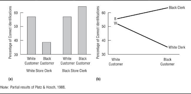
Partial results of Platz and Hosch, 1988.

Black and White clerks were equally accurate in identifying White customers, but Black clerks were more accurate in identifying Black customers. Whenever the lines on a line graph are not parallel there is an interaction effect.

However, as you can see from the percentages in Table 9.5 and the graphs in Figure 9.5, both of these conclusions would be wrong. In actuality, both race of the clerk and race of the customer were related to accuracy of identification: Clerks were more accurate in identifying members of their own race than members of the other race. However, White customers were identified with equal accuracy by White and Black clerks. Accuracy was determined neither by race of the clerk alone nor by race of the customer alone but, rather, by the unique combined effect, or interaction, of the variables.

The data from factorial experiments are analyzed using a form of ANOVA designed for this purpose. The ANOVA provides a test of the statistical significance of each main effect and interaction. If the interaction effect is not significant, the results of the experiment can be interpreted as if two experiments were conducted, one with each of the independent variables. If the interaction effect is significant, the interpretation of the results becomes more complex.

Outcomes of factorial designs. There are eight possible outcomes of a 2 × 2 factorial design: There may or may not be an effect for the first independent variable, there may or may not be an effect for the second independent variable, and the independent variables may or may not interact. Examples of these outcomes are illustrated in Figure 9.6, which uses a hypothetical experiment with aggression as the dependent variable and sex of participant and whether or not the participants have a frustrating experience as the independent variables. These results are completely fictitious; they do not illustrate the results of any real experiments. However, they do provide good concrete illustrations of the possible outcomes of a 2 × 2 experiment. Each panel in Figure 9.6 has two parts: a table of means and a graph of those means. The first four panels illustrate situations in which there is no interaction. In panel (a), neither independent variable has an effect, in panels (b) and (c), only one independent variable has an effect, and in panel (d), both independent variables have effects. Panels (e), (f), and (g) illustrate outcomes that include both main effects and interactions. Panel (h) illustrates a situation in which there is an interaction but no main effects. Note that whenever there is an interaction, the lines in the graph are not parallel.

Interaction Effects

Factorial designs are quite common in behavioral science research, and they frequently reveal interaction effects. These effects can be difficult to interpret. Let’s look first at the ways of displaying interaction effects in research reports and then at how to go about interpreting them.

Displaying interactions. The results of a factorial experiment can be displayed either in the form of a table, as in Table 9.5 and Figure 9.6, or in the form of a graph, as in the examples in Figures 9.5 and 9.6. A tabular display typically takes the form of a matrix, with each cell in the matrix representing one combination of the independent variables. For example, the upper left-hand cell in Table 9.5 represents what happened when White clerks were asked to identify a White customer. The decision about which independent variable goes across the top of the matrix and which goes along the side is essentially arbitrary; the placement that most clearly illustrates the results is normally used. The main effects—the means of the conditions of one independent variable averaged across the conditions of the other independent variable—can be displayed at the bottom and right edge of the table as shown in Table 9.5.

When the independent variables are qualitative variables, as in the Platz and Hosch (1988) experiment, the results can be graphed in the form of a histogram, as in panel (a) of Figure 9.5. For quantitative independent variables and qualitative variables in simpler factorial designs, a line graph can be used, as in panel (b) of Figure 9.5 and in Figure 9.6. In the line graph format, the conditions of one independent variable are arranged along the horizontal (X) axis—race of customer in Figure 9.5(b) and frustration level in Figure 9.6—and the means for each combination of conditions of the independent variables are plotted using the vertical (Y) axis for the dependent variable. Lines connect the points within conditions of the second independent variable.

FIGURE 9.6

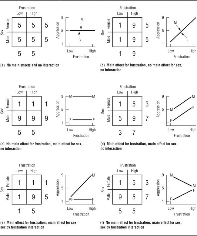
Possible Outcomes of a 2 × 2 Factorial Design.

Interpreting interactions. When interpreting interaction effects, it can be useful to think of a piece of research as a question. The question is “Does the independent variable have an effect on the dependent variable?” When the outcome is one or more main effects without an interaction, the answer is a simple yes. When the outcome is an interaction, with or without main effects, the answer is “It depends”: The answer for one independent variable depends on the condition of the other independent variable. For example, in the Platz and Hosch (1988) study, one question was “Is a person’s race related to the accuracy with which the person can identify another person?” The answer, as we saw in Table 9.5 and Figure 9.5, is not a simple yes or no; it depends on the race of the other person. Black participants were more accurate in identifying Black people, and White participants were more accurate in identifying White people. The other question asked by the Platz and Hosch study was “Does a person’s race affect how accurately that person is identified by someone else?” Again, the answer is “It depends,” this time on the race of the person making the identification. White people were identified with equal accuracy by Black and White participants, but Black people were more accurately identified by Black participants than by White participants.

The “it depends” nature of interactions has an important implication for understanding the research results: If the research produces an interaction, any main effects found may be deceptive, representing statistical artifact rather than a true main effect of the independent variable. Consequently, if the statistical analysis finds both a main effect and an interaction, the main effect for one independent variable may apply only to one condition of the other independent variable, not to both conditions. For example, Figure 9.6(e) illustrates a situation in which there are two main effects—the average aggression score for men is higher than that for women and higher for participants in the high-frustration condition than for those in the low-frustration condition—and an interaction—men who experienced high frustration were more aggressive than the participants in any of the other conditions. Notice, however, that sex of participant is related to aggression only in the high-frustration condition; there is no sex difference in the low-frustration condition. Similarly, differences in frustration lead to differences in aggression only for men; women respond to both high and low frustration with the same level of aggression.

FIGURE 9.7

Hypothetical Experimental Results Illustrating the Presence of Both an Interaction and a True Main Effect.

The effect of frustration is different for men and women, but men score higher than women regardless of frustration level.

However, sometimes there can be both an interaction and a true main effect. Figure 9.7 illustrates this situation. In this hypothetical outcome of a frustration-aggression experiment, women’s aggression is, as in the last example, still unaffected by level of frustration and men’s aggression increases with level of frustration. However, unlike Figure 9.6(e), men are more aggressive than women in both the high-and low-frustration conditions. Thus, men are more aggressive overall than are women and men’s aggression is influenced by level of frustration whereas women’s aggression is not.

When there is an interaction but no main effects, the effect of one independent variable in one condition of the second independent variable is reversed in the other condition of the second independent variable. This phenomenon can be seen in the results of a study conducted by Fazio, Cooper, Dayson, and Johnson (1981). One independent variable in their study was the personality type of their participants, Type A or Type B. One characteristic of Type A people is that they find it easier to ignore stress than do Type B people. The other independent variable was the degree of stress that the participants underwent while they performed a proofreading task. The dependent variable was the number of lines the participants could proof in a given amount of time. The results of the study are shown in Figure 9.8. Type A people performed better under high stress than under low stress, whereas Type B people performed better under low stress than under high stress: Stress had opposite effects on performance depending on personality type.

When you face a significant interaction effect in a factorial design, you are in a position much like that which occurs when you find a significant F value in a multiple group design: there is a significant difference somewhere among the means, but you do not yet know where the difference or differences lie. Again, the solution is to conduct post hoc comparisons if the hypothesis did not predict a particular form of interaction. If the hypothesis did specify a particular outcome, then a priori contrasts should be used. For example, a replication of the Platz and Hosch (1988) study would hypothesize that people would make more accurate identifications of members of their own races. This hypothesis would be tested statistically by grouping research participants by race and comparing their accuracy in identifying members of their own and other races. Most statistics textbooks discuss the use of both a priori and post hoc contrasts in factorial designs.

FIGURE 9.8

Quality of Task Performance Was an Interactive Function of Stress and Personality Type.

Forms of Factorial Designs

Factorial designs can take a number of forms, depending on whether the independent variables are manipulated in a between-subjects or within-subjects format, whether the independent variables are manipulated or measured, the number of independent variables, and the number of conditions of the independent variables.

Between-and within-subjects designs. The independent variables in a factorial design can be between-subjects variables, or within-subjects variables, or a combination of the two. The two most common designs are probably completely between-subjects designs and mixed between-within designs. Platz and Hosch (1988), for example, used a mixed between-within design. Race of store clerk was the between-subjects variable. Race of customer was manipulated as a within-subjects variable by having both a White customer and a Black customer interact with each clerk, and each clerk was asked to identify the Black customer from a set of photographs of Black men and the White customer from a set of photographs of White men. Platz and Hosch counterbalanced the order in which the customers dealt with the clerk and the order in which the clerks saw the sets of photographs. The between-within procedure allowed Platz and Hosch to use fewer store clerks as research participants than a completely between-subjects design would have required. This economy was necessary because the stores that gave their permission to be used for the research employed only one quarter as many Black clerks as White clerks. The within-subjects aspect of the design also allowed the researchers to control for possible individual differences in the clerks’ abilities to remember faces. Because each clerk interacted with both a Black customer and a White customer, differences in memory ability could not be accidentally confounded with race of customer. Special forms of ANOVA are required for the analysis of data from mixed between-within designs. If you plan to conduct such a study, consult a statistics text to ensure that you understand those procedures.

Manipulated and measured independent variables. The independent variable in a true experiment is manipulated by the experimenter. However, researchers are often interested in variables, such as personality traits, that cannot be manipulated but can only be measured, and in the interactions between measured and manipulated variables. Consequently, one frequently sees research using factorial designs in which at least one of the independent variables is measured rather than manipulated. For example, Fazio et al. (1981) manipulated level of stress but measured personality type; Platz and Hosch (1988) manipulated race of customer but measured race of clerk. As noted in Chapter 2, measured independent variables result in correlational rather than experimental research. Mixed experimental-correlational designs such as those used by Fazio et al. and by Platz and Hosch can be quite useful, but be careful in interpreting their results. Remember that correlational research can never determine whether changes in the level or condition of an independent variable cause changes in a dependent variable; it can determine only if a relationship exists between the variables. Therefore, be careful never to interpret the results of the correlational part of a mixed correlational-experimental study as indicating causality. For example, Fazio et al. could not correctly say that personality type caused differences in performance on the research task, only that it was related to those differences. However, because they manipulated level of stress, they could legitimately say that stress caused differences in performance.

It is also possible to have factorial designs in which all the independent variables are correlational. For example, McFatter (1994) examined the relationships of two personality characteristics—introversion-extraversion and neuroticism—to mood. He noted that most previous research had examined the separate relationship of each variable to mood but that little research had considered both in the same study. McFatter found an interaction between introversion-extraversion and neuroticism: Neurotic introverts reported less positive mood and more negative mood than did people with other combinations of the traits. In this case, of course, McFatter could not interpret his findings in causal terms. When scores on the measured variable are continuous, multiple regression analysis (see Chapter 11) is the best choice for data analysis; this procedure provides the same information as an ANOVA, including about the effects due to any categorical independent variables and the interactions between the variables of interest, but is not subject to the biases (discussed in Chapter 11) that can result from dichotomizing a continuous variable (see also Judd, 2000).

Design complexity. The examples of factorial designs used so far have all been 2 × 2 designs. However, in principle there is no limit on the number of independent variables one can have or on the number of levels or conditions per independent variable. For example, although we have looked at the Platz and Hosch study as a 2 × 2 design, they actually used a 3 × 3 design: They included Hispanic customers and clerks as well as Black and White customers and clerks. Sprecher, McKinney, and Orbuch (1987) used a 2 × 2 × 2 × 2 design to investigate the factors that influence people’s evaluation of other people whom they learn are sexually active. The independent variables were the sex of the person being evaluated, the age of the person (16 or 21), the type of relationship in which the sexual behavior took place (casual or close), and sex of the research participant.

Although there is no theoretical limit on the number of independent variables or number of conditions, studies rarely use more than three independent variables or three conditions per independent variable. The reason for this limitation is practical: The total number of conditions in the study increases quickly as the number of independent variables and number of conditions per independent variable increase. For example, as shown in Figure 9.6, a 2 × 2 design has a total of four conditions: all the possible combinations of the two conditions of each of the two independent variables. A 3 × 3 design, such as Platz and Hosch’s (1988), has 9 conditions, and a 2 × 2 × 2 × 2 design, such as Sprecher et al.’s (1987), has 16 conditions. Note that the total number of conditions is the product of the number of conditions of the independent variables: 2 × 2 = 4, 3 × 3 × = 9, 2 × 2 × 2 × 2 = 16, and so forth. As the total number of conditions increases, the number of research participants needed in a between-subjects design increases: With 10 participants per condition, a 2 × 2 design requires 40 participants but a 2 × 2 × 2 × 2 design requires 160. In addition, the complexity of the data analysis and of the interpretation of the results of that analysis increases. Consequently, most researchers limit themselves to relatively simple designs.

Uses for Factorial Designs

Factorial designs are fairly complex, requiring two or more independent variables and multiple groups of participants, one group for each combination of the independent variables. Why should you bother with this complexity when you can determine the effect of an independent variable with a simpler design? Factorial designs can be used to test hypotheses about moderator variables, to detect order effects in counterbalanced within-subjects designs, and to control extraneous variance by a technique called blocking.

Testing moderator hypotheses. The discussion of the “it depends” nature of interactions probably reminded you of the discussion of moderator variables in Chapter 1. As you recall, a moderator variable changes the effect of an independent variable: The effect of the independent variable is different under different conditions of the moderator variable. Thus, in the Platz and Hosch (1988) study, you could say that race of the store clerk moderated the effect that race of the customer had on accuracy of identification. You could also look at it the other way and say that race of the customer moderated the relationship between race of the clerk and accuracy of identification. The variable you consider the moderator variable depends on your frame of reference—that is, on which variable you conceptualize as the independent variable being studied and which as the moderator variable influencing the effect of the independent variable. If you are testing a theory, the theory often provides the frame of reference, designating which variables are independent variables and which are moderator variables. Note, however, that because the effect of a moderator variable takes the form of an interaction, the hypothesis that one variable moderates the effect of another can be tested only with a factorial design and will be supported only if the predicted interaction is found.

Detecting order effects. Order effects present a potential threat to the validity of the conclusions that can be drawn from the research using within-subjects designs. When the order of conditions is counterbalanced, researchers can detect the presence and size of order effects by using a between-within factorial design, with the independent variable being tested as the within-subjects factor and order of conditions (experimental before control and control before experimental) as the between-subjects factor. Some possible outcomes of this procedure are shown in Table 9.6. The top panel shows an outcome in which the independent variable had an effect and there was no order effect. In this case, there will be a main effect for the independent variable (the mean for the experimental condition is 10 points greater than the mean for the control condition), no main effect for the order factor (the two order means are equal), and no interaction effect. The middle panel shows the outcome for the same experiment when there is an order effect that is the same for both orders. There is a main effect for the independent variable and no order effect, but there is an interaction between the conditions of the independent variable and the order in which participants experienced the conditions. In this case, experiencing a condition as the second condition added 10 points to the participants’ scores. Because the order effect happens to be the same as the effect of the independent variable, there is no difference between the means in the experimental and control conditions for participants who experienced the experimental condition first, and an exaggerated difference for those who experienced the control condition first. Note, however, that because the order effect was the same for both orders, the difference between the means for the experimental and control conditions reflects the true difference between the means. The bottom panel of Table 9.6 shows the outcome with a differential order effect, in which experiencing the control condition second added 10 points to a person’s score, whereas experiencing the experimental condition second added 20 points. In this case, there are main effects for both the independent variable and order, as well as an interaction between the two. Note also that the difference in means in the experimental and control conditions is greater than the true difference shown in the top panel.

TABLE 9.6

Use of Between-Within Designs to Detect Order Effects

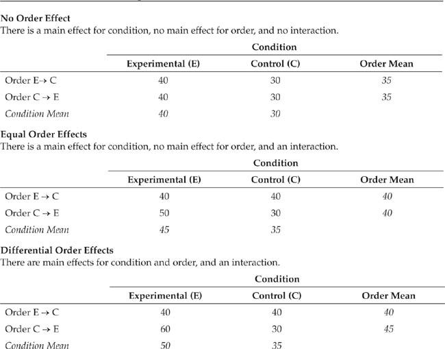
Although order effects contaminate one’s data, all is not lost. Note that order effects do not affect the scores in the condition that participants experience first. Consequently, one can analyze the experimental and control data from the experimental-first and control-first participants as a between-subjects design and still test the hypothesis. The cost of this procedure is the loss of the advantages of a within-subjects design, but the benefit is the ability to draw valid conclusions from the data. Order effects are always potential threats to the validity of within-subjects designs, so researchers should always test to see if these effects are contaminating their data.

Blocking on extraneous variables. Recall that from a statistical point of view any variance not attributable to an independent variable is error variance and that extraneous variables are one source of such variance. One way in which researchers can deal with the effects of extraneous variables is to include them as independent variables in a factorial design. A factorial ANOVA will remove the variance due to the extraneous variable and its interaction with the independent variable from the error variance and treat it as variance due to an independent variable and to the interaction of two independent variables. This procedure can reduce the error variance and so increase the sensitivity of the statistical test of the effect of the independent variable. Consider the data presented in the top panel of Table 9.7, which come from a hypothetical experiment in which the researcher ensured that equal numbers of men and women participated in the experimental and control conditions. The experimental group had a mean score of 16.9 and the control group had a mean score of 14.2; however, as shown by the statistical analysis in the middle panel of the table, this difference was not statistically significant.

TABLE 9.7

Effect of Blocking on an Extraneous Variable on Statistical Analysis

Blocking increases the sensitivity of the statistical test by reducing the error variance.

Scores

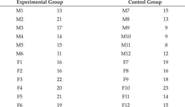
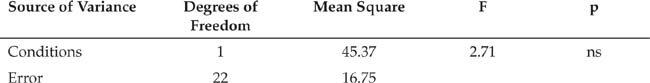
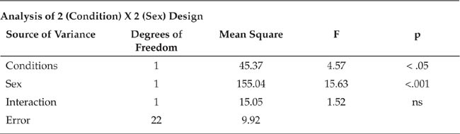
Note: M = male participants, F = female participants.

The statistical analysis shown in the bottom panel of the table shows what happens when the participants are blocked on sex. Blocking means that the participants are grouped according to an extraneous variable and that variable is added as a factor in the design. The new analysis finds significant effects for both the independent variable and for participant sex, with women, who had a mean score of 18.1, performing better than men, who had a mean score of 13.0.

The numbers in the “Mean Square” columns in the middle and bottom panels of Table 9.7 represent the amount of variance in the dependent variable attributable to each factor in the design, including error. The bottom panel shows that participant sex accounted for much more variance in the dependent variable than did the independent variable. As illustrated in Figure 9.9, this variance, along with the nonsignificant variance accounted for by the interaction, was treated as part of the error variance in the analysis shown in the middle panel, increasing the size of the error variances. The variance attributable to the independent variable is the same in both analyses. Because the F-test is the ratio of the variance due to an independent variable to the error variance, the F value in the middle panel is smaller than that in the bottom panel. An experimenter who ignored the effect of participant sex as an extraneous variable would incorrectly conclude that the independent variable had no effect on the dependent variable.

When conducting your literature review for a research project, it is extremely important to identify extraneous variables so that you can take steps to control them. A major advantage of the use of an extraneous variable as a factor in a factorial design is that it becomes possible to determine if the extraneous variable interacts with the independent variable. The alternative methods of control, such as holding the extraneous variable constant across conditions of the independent variable, ignore its possible moderating effects and, as we discussed in Chapter 8, they also limit the interpretations you can make about the generalizability of the research results. However, use blocking with care: It operates to reduce error variance only when the blocking variable has a strong effect on or is highly correlated with the dependent variable. Under other conditions, blocking could actually increase the error variance by decreasing the degrees of freedom associated with the error term.

FIGURE 9.9

Blocking Reduces the Error Term for Statistical Analyses.

When the variance due to sex and the sex by condition interaction is “pulled out” of the error term by blocking on sex, then the size of the error term is reduced, increasing the likelihood of statistical significance for the F-test.

Chapter Summary

Five aspects of experimental research are considerations in manipulating the independent variable, ways of controlling unwanted variance in the dependent variable, the functions of control groups, and the use of multiple-group and factorial experiments. Inferential statistics assist the research process by partitioning participants’ scores on the dependent variable into treatment variance caused by the independent variable and error variance caused by extraneous variables. Two goals of research design are increasing treatment variance and reducing error variance.

Every experiment has at least one experimental condition and at least one control or comparison condition. The most basic function of a control condition is to provide a baseline against which to assess the effects of the independent variable. However, additional control conditions might be needed to fully test the hypothesis being studied or to rule out alternative explanations for the predicted effects of the independent variable.

Manipulations of independent variables must be valid, reliable, strong, and salient. Manipulation checks are used to test the construct validity of a manipulation. Reliable manipulations are consistently applied to all participants. Strong manipulations serve to increase treatment variance. Salient manipulations are noticeable by participants. When the stimuli used for a manipulation are samples from a population of possible stimuli, multiple stimuli should be used in each condition of the experiment. This procedure allows one to separate the effects of the construct being measured from the effects of the unique properties of the stimuli.

Extraneous variables are characteristics of the research situation and participants that add unwanted (error) variance to the dependent variable. Experimenters control the effects of situational extraneous variables by holding those variables constant for all participants, thereby spreading their effects evenly across the conditions of the experiment. Extraneous variables that are characteristics of the research participants can be dealt with in five ways. Some characteristics, such as sex of participant, can be held constant. Researchers can balance the effects of other characteristics across conditions by randomly assigning participants to conditions, matching participants on key characteristics and randomly assigning the members of matched pairs to conditions, or by using a within-subjects design. Finally, participants can be blocked on a characteristic and the characteristic can be treated as an independent variable in a factorial design.

Simple random assignment and matched random assignment of participants to conditions are used in between-subjects designs, in which a participant experiences only one condition of the independent variable. In within-subjects designs, each participant experiences each condition of the independent variable, thereby providing a perfect “match” between the participants in the conditions. This procedure reduces error variance and requires fewer participants than an equivalent between-subjects design. However, order effects—practice, carryover, and sensitization—can threaten the internal validity of a within-subjects experiment. Counterbalancing the order of conditions can spread these effects across conditions, and using a washout period can control carryover effects. When order is counterbalanced, a factorial design that includes order as a factor can detect order effects and determine if they are equal across orders.

Experiments can include more than one level of a quantitative independent variable or more than one category of a qualitative independent variable. Such a multiple-group design is the only way to determine if a quantitative independent variable has a curvilinear relationship to the dependent variable. Be careful, however, to conduct the appropriate follow-up statistical tests to determine which of the several possible differences among the means are statistically significant.

A factorial design has more than one independent variable. Factorial designs provide information about main effects (the separate effects of each independent variable) and interactions (the joint effect that two or more independent variables have over and above their main effects). Researchers must take care when interpreting the results of factorial experiments that find interaction effects because such effects indicate that the effect of one independent variable is different under different conditions of the other independent variable. Factorial designs can be within-subjects, or between-subjects, or a combination of the two. One or more factors can also be measured variables, but the results found for these variables cannot be interpreted in causal terms. Factorial designs can be used to test the effects of hypothesized moderator variables, to detect order effects in within-subjects designs, and to control the effects of extraneous variables.

Suggestions for Further Reading

Kirk, R. E. (1995). Experimental design: Procedures for the behavioral sciences (3rd ed.). Pacific Grove, CA; Brooks-Cole.

This classic book covers the statistical issues relevant to analysis of data from factorial designs. The text includes chapters on the assumptions of ANOVA and provides detailed information about analyzing simple and complex factorial designs. The strength of this text is that it is both comprehensive and accessible.

Gravetter, F. J., & Forzano, L-A. B. (2012). Research methods for the behavioral sciences (4th ed.). Belmont, CA: Wadsworth.

This well-regarded undergraduate text includes separate chapters on between- (Chapter 8) and within-subject (Chapter 9) experimental designs. The authors address the strengths and weakness of each design and discuss applications and statistical analysis of data from studies of each method. Potential threats to validity with each type of design are also addressed. Chapter 11 provides an overview of interpreting results of factorial designs.

Smith, E. R. (2000). Research design. In H. T. Reis, & C. M. Judd (Eds.). Handbook of research methods in social and personality psychology (pp. 17–39). Cambridge, United Kingdom: Cambridge University Press.

This chapter offers practical advice about experimental design. Issues discussed relevant to this chapter include fixed and random factors, creating powerful and meaningful levels of independent variables, choosing between within- and between-subjects designs, and controlling for order effects. Smith also considers construct, statistical conclusion, and external validity within the context of factorial designs.

Wilson, T. D., Aronson, E., & Carlsmith, K. (2010). The art of laboratory experimentation. In S. T. Fiske, D. T. Gilbert, & G. Lindzey (Eds.). Handbook of social psychology (5th ed., Vol. 1, pp. 51–81). Hoboken, NJ: Wiley.

Written with beginning graduate students in mind, this chapter focuses on laboratory experimentation broadly, addressing many issues discussed elsewhere in the current textbook. Relevant to this chapter is the discussion of (a) constructing independent variables that maximize their impact; (b) choosing the optimal number of levels for the independent variable; and (c) whether a between-or within-subject design is best suited for the proposed experiment.

Key Terms

A priori contrasts

Between-subjects design

Blocking

Carryover effects

Counterbalancing

Curvilinear relationship

Differential order effect

Error variance

Extraneous variable

Factorial design

Fatigue effects

Independent groups design

Interaction effect

Latin square design

Linear relationships

Main effect

Manipulation check

Matched random assignment

Moderator variable

Multiple group design

Negative relationship

Non-specific treatment effects

Order effects

Placebo effects

Positive relationship

Post hoc analysis

Practice effects

Repeated measures design

Salient manipulation

Sensitization effects

Simple random assignment

Stimulus

Strong manipulation

Treatment variance

Washout period

Within-subjects design

Questions for Review and Discussion

1.	What are the three defining characteristics of the experiment? How do correlational studies and case studies differ from experiments? (Review Chapter 2)
2.	Describe the purposes of control and comparison conditions in an experiment.
3.	What are the characteristics of a good manipulation? What problems do you think might arise in attempting to maximize these characteristics?
4.	Choose three recently published experiments on topics that interest you. How did each group of researchers manipulate their independent variables? Based on the criteria discussed in the chapter, how good do you think these manipulations were? What are your reasons for your evaluations?
5.	How can manipulation checks be conducted? What do you see as the advantages and disadvantages of each approach? Describe the factors that can result in a failed manipulation check.
6.	Describe the advantages of using multiple stimuli in research. Describe some research situations in which the use of multiple stimuli would be appropriate. How would the failure to use multiple stimuli when appropriate limit the conclusions that could be drawn from a study?
7.	Describe the ways in which an experimenter can control extraneous variance. What do you see as the advantages and disadvantages of each?
8.	How do within-subjects designs and between-subjects designs differ? Describe the advantages and disadvantages of within-subjects designs relative to between-subjects designs. Describe the steps an experimenter can take to overcome these disadvantages.
9.	Look again at the three studies that you chose for Question 4. Did each use a between-subjects design, a within-subjects design, or a mixed design? For each study, describe how the between-subjects factors could be manipulated as within-subjects factors and how the within-subjects factors could be manipulated as between-subjects factors. What benefits would accrue and what problems would arise from the changes in each case?
10.	What advantages do multiple-group experiments have over two-group experiments? Describe the problems in interpreting the results of multiple-group experiments.
11.	For each of these factorial designs, what are the number of independent variables, the number of conditions of each independent variable, and the total number of conditions?

a. 2 × 2

b. 3 × 2

c. 3 × 2 × 2

d. 4 × 3 × 2 × 2

12.	Describe the possible outcomes of a 2 × 2 factorial design. If the results of a factorial experiment show both an interaction and a main effect, how should the main effect be interpreted?
13.	What advantages do factorial designs have over designs that include only one independent variable? What can factorial designs do that the other designs cannot?
14.	Choose three recently published experiments on topics that interest you that used factorial designs. In each case, were the factors all between-subjects, all within-subjects, mixed between and within, or mixed experimental and correlational? In your opinion, did the researchers properly interpret the results of their studies? What are your reasons for your answer?

Order of Conditions
Basic Design					Balanced Design
1	A	B	C	D	1	A	B	C	D
2	B	C	D	A	2	B	D	A	C
3	C	D	A	B	3	C	A	D	B
4	D	A	B	C	4	D	C	B	A