The Nature of Correlational Research
Assumptions of Linearity and Additivity
Factors Affecting the Correlation Coefficient
Simple and Partial Correlation Analysis
Multiple Regression Analysis (MRA)
The multiple correlation coefficient
The Problem of Multicollinearity
Dealing with multicollinearity
MRA as an Alternative to ANOVA
Continuous independent variables
Correlated independent variables
Some Other Correlational Techniques
Suggestions for Further Reading
Questions for Review and Discussion
Although the experiment is the only research strategy that can determine if one variable causes another, not all phenomena of interest to behavioral scientists can be studied experimentally. For example, it is impossible to manipulate some factors, such as personality, that behavioral scientists would like to study as independent variables. If manipulation is not possible, then neither is experimentation. In other cases, it might be unethical to manipulate a variable. For example, researchers might want to conduct an experimental study of the effects of long-term exposure to severe stress. Although such an experiment would be possible, it would raise ethical concerns about harm to the participants.
Most variables that cannot be studied experimentally can be studied correlationally. Even though personality traits cannot be manipulated, they can be measured and the degree to which they are related to other variables, such as behaviors, can be determined. Even though it is not ethical to intentionally subject people to long-term, severe stress, it is possible to locate people who experience different degrees of stress, some of it severe, as part of their everyday lives and to correlate degree of stress with outcome variables such as frequency of illness.
As noted in Chapter 2, the major drawback to the correlational research strategy is that it cannot determine whether one variable causes another. Although correlational research can determine if two variables covary—the first requirement for causality—it cannot always establish time precedence of the presumed cause and cannot rule out all alternative explanations for any relationships found. Yet correlational research can show that one variable does not cause another: Because the covariance of two variables is an absolute requirement for causality, lack of a correlation can demonstrate a lack of causality.
This chapter provides an overview of correlational research. We first note some assumptions underlying correlational research methods and some factors that can have unwanted effects on correlation coefficients. We then outline the principal methods of correlational research—simple correlation, partial correlation, and multiple regression analysis. The chapter concludes with brief discussions of two other forms of correlational analysis you might encounter—logistic regression analysis and multiway frequency analysis.
But first, a note on terminology: Throughout this chapter we use the term independent variable to refer to the variable or variables in a correlational study that the theory being tested presumes is the causal variable or variables. This term is, to some degree, misleading because independent variable is frequently used to refer only to the manipulated variables in experiments. However, researchers conducting correlational studies usually assume that one variable or a set of variables causes another, which we call the dependent variable. We use these terms as a matter of convenience and do not intend to imply that correlational research can determine causality.
Correlational research can be carried out in a number of ways. However, several issues are involved in all forms of correlational research. This section discusses three of those issues: the assumptions of linearity and additivity, factors that affect the size of a correlation coefficient found in a study, and the multifaceted nature of some constructs.
As noted in Chapter 9, all statistical tests are based on assumptions. Two of the assumptions underlying correlational statistics are that the relationship between the variables is linear and that there are no interactions present when multiple independent variables are studied.
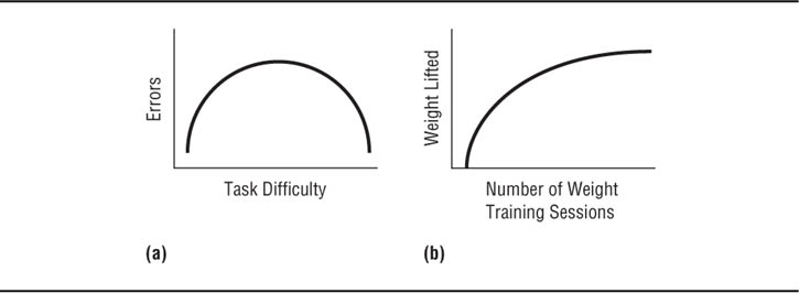
Linearity. Generally, the use of correlational research methods assumes that the relationship between the independent and dependent variables is linear that is, that the relationship can be graphed as a straight line. Curvilinear relationships cannot be detected by simple correlational methods. For example, the correlation coefficient for the relationship illustrated in panel (a) of Figure 11.1 would be zero, even though the scores on the two variables are clearly related. A more subtle problem is illustrated in panel (b) of Figure 11.1, which shows a relationship between two variables that is initially linear and positive but eventually becomes zero. In this case the correlation coefficient for the two sets of scores will be positive. However, because the relationship is not completely linear, the coefficient will be misleading; that is, it will not reflect the true relationship between the variables. As a general rule, one should plot the relationship between the scores on two variables before conducting a correlational analysis in order to ensure that the relationship is linear. If there is reason to suspect a curvilinear relationship between the independent and dependent variables in a study, simple correlational analysis is not appropriate.
Additivity. Correlational analyses involving more than one independent variable also generally assume that the relationship between the independent and dependent variable is additive. That is, people’s scores on the dependent variable can be predicted by an equation that sums their weighted scores on the independent variables. For example, Schuman, Walsh, Olson, and Etheridge (1985) used total Scholastic Assessment Test (SAT) scores, self-reported average number of hours of study per day (HOURS), and self-reported percentage of classes attended (ATTEND) to predict grade point average (GPA) for college students. They found that the formula GPA = 1.99 + .0003 x SAT + .009 x HOURS + .008 x ATTEND predicted 13.5% of the variance in GPA. Another way of looking at the assumption of additivity is that it presumes there are no interactions among the independent variables. This means that Schuman et al. assumed that, for example, class attendance had the same relationship to GPA regardless of SAT scores; that is, they assumed that cutting class had the same effect on the grades of students with high SAT scores as it did on the grades of students with low SAT scores. Although interaction effects cannot be tested using simple correlation analysis, they can be tested using multiple regression analysis, which is discussed later in this chapter.
Examples of Curvilinear Relationships.
Even given a linear relationship between two variables, several aspects of the instruments used to measure the variables, the distributions of scores on the variables, and the participant sample can affect the observed correlation. Low reliability and restriction in range lead to underestimates of the population value of a correlation, and outliers and differences in subgroup correlations can dramatically affect the size of the correlation coefficient.
Reliability of the measures. The relationship between the true scores of two variables is called their true score correlation; the relationship a study finds is called their observed correlation. The observed correlation is an estimate of the true score correlation; its value is not necessarily equal to that of the true score correlation. All else being equal, the more reliable the measures of the two variables (the less random error they contain), the closer the observed correlation will be to the true score correlation. As the measures become less reliable, the observed correlation will underestimate the true score correlation. The relationship between reliability and the size of the observed correlation is rxy = rXY  where rxy is the observed correlation, rXY is the true score correlation, and rxx and ryy are the reliabilities of the measures. For example, with a true score correlation of .55 and two measures with reliabilities of .80, the maximum possible observed correlation is .44. This shrinkage of the observed correlation relative to the true score correlation is called attenuation. Thus, it is imperative to use the most reliable available measures when conducting correlational research. The same principle applies, of course, to experimental research. However, because the reliability of a carefully manipulated independent variable should approach 1.00, the attenuation of the observed relationship relative to the true score relationship is greatly reduced. Nonetheless, an unreliable measure of the dependent variable can lead to underestimates of the size of its relationship to the independent variable.
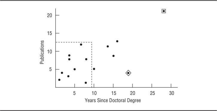
Restriction in range. Restriction in range occurs when the scores of one or both variables in a sample have a range of values that is less than the range of scores in the population. Restriction in range reduces the correlation found in a sample relative to the correlation that exists in the population. This reduction occurs because as a variable’s range narrows, the variable comes closer to being a constant. Because the correlation between a constant and a variable is zero, as a variable’s sampled range becomes smaller, its maximum possible correlation with another variable will approach zero, that is, become smaller. Consider the data in Table 11.1, which show the number of years since the award of the doctoral degree and total number of publications for 15 hypothetical professors, and Figure 11.2, which shows a scatterplot of those data. The correlation between the two variables is .68; however, if only those professors with less than 10 years of experience are considered (shown by the dashed line in Figure 11.2), the correlation is reduced to .34.
Hypothetical Data for the Correlation of Years since Doctorate with Number of Publications
Case |
Years |
Publications |
1 |
1 |
2 |
2 |
2 |
4 |
3 |
5 |
5 |
4 |
7 |
12 |
5 |
10 |
5 |
6 |
4 |
9 |
7 |
3 |
3 |
8 |
8 |
1 |
9 |
4 |
8 |
10 |
16 |
12 |
11 |
15 |
9 |
12 |
19 |
4 |
13 |
8 |
8 |
14 |
14 |
11 |
15 |
28 |
21 |
Note: Adapted from Cohen, Cohen, West, and Aiken (2002)
Scatterplot of Data from Table 11.1.
Restriction in range is especially likely to be a problem when research participants are selected on the basis of extreme scores on one of the variables or if the participant sample is drawn from a subgroup of the population that has a natural restriction in range on a variable. For example, studies of the concurrent validity of employment selection tests correlate the test scores of people already on the job with measures of job performance. Because only good performers are likely to be hired and remain on the job, their job performance scores, and possibly their test scores, are restricted to the high end of the range. College students provide an example of a subpopulation with a natural restriction in age range, with most being 18 to 22 years old. Correlations between age and other variables may therefore be deceptively low when college students serve as research participants.
Outliers. Outliers are extreme scores, usually defined as being scores more than three standard deviations above or below the mean (Tabachnick & Fidell, 2007). The influence of outliers can be seen in the data in Table 11.1 and Figure 11.2. Notice that Case 15 (shown in a square in Figure 11.2) has unusually high values for both variables—28 years since doctorate and 21 publications—and so lies well outside the scatterplot of cases. If Case 15 is removed from the data set, the correlation between years since doctorate and publications becomes .38; Case 15’s unusually high values on both variables inflated the correlation. Outliers can also artificially lower a correlation. Consider Case 12 (shown in a diamond in Figure 11.2), which has an unusually low number of publications (4) given the number of years since doctorate (19) compared to the rest of the cases. If Case 12 is removed from the data set along with Case 15, the correlation becomes .60.
The example just used illustrates the detection of outliers by inspection; that is, by looking at the distribution of scores on a variable or at a scatterplot of the relationship between two sets of scores. However, if a study includes more than two variables, inspection might not be sufficient to detect outliers because they might be the result of a combination of three or more variables. Tabachnick and Fidell (2007) describe statistical procedures that can be used in these situations to detect outliers.
What should you do about outliers? Tabachnick and Fidell (2007) suggest transforming the data mathematically, such as by using the logarithms of the scores, to remove the effects of outliers. However, in such a case the results of the statistical analysis related to the transformed scores rather than to the original scores, so their meaning may be unclear. Cohen, Cohen, West, and Aiken (2003) suggest omitting outliers from the data analysis, especially if there are only a few. In this case some data are lost. Ultimately, the decision about outliers rests with the researcher and must be based on the probable meaning of the outlying scores. For example, you might want to discard scores that most likely represent coding or other errors. Data sets with outliers that represent accurate data could be transformed to remove the effects of the outliers, or the outliers could be excluded from the data analysis but studied separately as special cases.
Subgroup differences. The participant sample on which a correlation is based might contain two or more subgroups, such as women and men. Unless the correlations between the variables being studied are the same for all groups and all groups have the same mean scores on the variables, the correlation in the combined group will not accurately reflect the subgroup correlations. For example, Whitley, Childs, and Collins (2011) examined African American and White college students’ attitudes toward lesbians and gay men. Using the combined scores of both groups, the researchers found a statistically significant correlation of r = -.29 between attitudes toward lesbians and racial identification, indicating that participants who scored higher on racial identification reported more negative attitudes. However, when computed separately for each group, the correlations were small and not statistically significant, r = -.11 for both groups. Why was the correlation for the combined scores so different from the subgroup correlations? Consider Figure 11.3, which presents the results schematically. The circles represent the near-zero subgroup correlations and the oblong represents the correlation for the combined scores. The larger combined score correlation was found because, on the average, White students, compared to African American students, scored higher on attitudes toward lesbians and lower on racial identification. Because of potential problems such as this one, it is always wise to examine subgroup means and correlations before analyzing the data for the combined group. One could also plot the subgroups’ scores on the variables on a single scatterplot, but unless the groups’ scores are plotted in different symbols or different colors, differences in the groups’ scatterplots may be difficult to pick out.
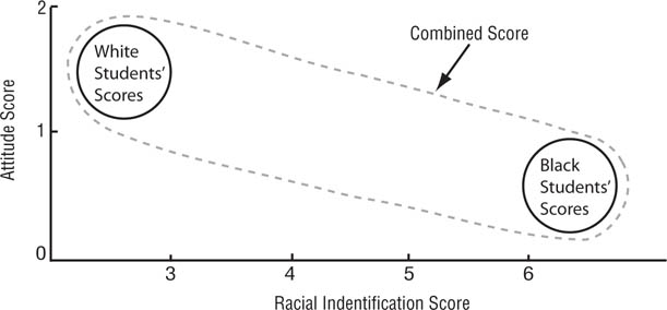
Schematic Representation of Effect of Considering Subgroup Differences When Interpreting Correlations.
There is almost no correlation between the variables within each group but because the groups have different mean scores on the variables, when their data are combined a correlation emerges.
As we noted in Chapter 1, Carver (1989) defined multifaceted constructs as constructs “that are composed of two or more subordinate concepts, each of which can be distinguished from the others and measured separately, despite their being related to each other both logically and empirically” (p. 577). An example of a multifaceted construct is attributional style (Abramson, Metalsky, & Alloy, 1989), which is composed of three facets: internality, stability, and globality. These facets are interrelated in that the theory holds that a person who attributes negative life events to causes that are internal, stable, and global is, under certain circumstances, more prone to depression and low self-esteem than a person who does not exhibit this attributional pattern. Not all multidimensional constructs are multifaceted in the sense used here. For example, the two components of the Ohio State leadership model (Stogdill & Coons, 1956), structure and consideration, are assumed to have independent effects on different aspects of leadership behavior. A test of whether a construct is multifaceted as opposed to one that is simply multidimensional is whether you (or other researchers) are tempted to combine the scores on the facets into an overall index. A major issue in research using multifaceted constructs is that of when facets should and should not be combined.
Keeping facets separate. There are three circumstances in which facets should not be combined. The first is when the facets are theoretically or empirically related to different dependent variables or to different facets of a dependent variable. For example, the attributional theory of depression holds that internality attributions are (under specific circumstances) related to self-esteem, stability attributions to the duration of depression, and globality attributions to the generality of depressive symptoms (Abramson et al., 1989). For the theory to be adequately tested, one must separately test the relationships of the facets of attributional style to their appropriate dependent variables (Carver, 1989). In addition, specific relationships between the facets of a construct and different dependent variables can be discovered empirically (see, for example, Snyder, 1986).
When the facets of a multifaceted construct are combined into a general index, useful information can be lost. For example, Crandall (1994) developed a scale to measure people’s attitudes toward fatness in other people, which he named the Antifat Attitudes Questionnaire. The questionnaire measures three facets of antifat attitudes: dislike of fat people, degree of belief that fatness is due to lack of willpower, and fear of becoming fat. Table 11.2 shows the correlations between total scores on the Antifat Attitudes Questionnaire, its three facets, and three other variables: the degree to which a person believes that people deserve whatever happens to them (belief in a just world), racist attitudes (modern racism), and the degree to which a person defers to authority figures (authoritarianism). As you can see, belief in a just world and racist attitudes have positive correlations with the total antifat attitude score and the dislike and willpower facets, but have no correlation with the fear-of-fat facet. In contrast, authoritarianism is uncorrelated with both the total score and with the willpower facet, but has a positive correlation with the dislike facet and a negative correlation with the fear-of-fat facet. Focusing solely on the relationships of the total antifat attitude score with the scores on the other variables would give an inaccurate picture of the true pattern of relationships, which are shown by the correlations involving the facet scores. Therefore, unless you are certain that the combined score on a construct and the scores on all the facets have the same relation to a dependent variable, test both the combined score and the facet scores to derive the most accurate information from your research.
The second circumstance in which you should avoid combined scores is when the theory of the construct predicts an interaction among the facets. Carver (1989) pointed out that the attributional theory of depression can be interpreted as predicting an interaction among the facets: A person becomes at risk for depression when negative events are consistently attributed to causes that are internal and stable and global. That is, all three conditions must be simultaneously present for the effect to occur, which represents an interaction among the facets. If facets are combined into a single score, it is impossible to test for their interaction. Finally, facets should not be combined simply as a convenience. Although dealing with one overall construct is simpler than dealing with each of its components, the potential loss of useful information described earlier far outweighs the gain in simplicity.
Correlation Between an Overall Measure and the Three Facets of Antifat Attitudes and Three Other Variables
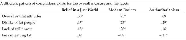
* p < .05.
Note: Facet correlations from Crandall (1989); overall correlations courtesy of Professor Crandall.
Combining facets. When, then, can researchers combine scores across facets? One circumstance is when a researcher is interested in the latent variable represented by the combination of facets rather than in the particular aspects of the variable represented by the facets. A latent variable is an unmeasured variable represented by the combination of several operational definitions of a construct. For example, the latent variable of depression has at least three facets: mood, symptoms, and surface syndrome (Boyle, 1985). A research question, such as whether depression (as a hypothetical construct rather than as measured in any one manifestation) is related to a dependent variable such as aggression, could be tested by correlating a depression index made up of scores on the three facets of depression with a measure of aggression, which could also be an index made up of scores from measures of several facets of aggression. Although interest in the latent variable is a justification for combining across facets, bear two cautions in mind. First, if the latent variable is more important in relation to the dependent variable than any of its facets, it should be a better predictor of the dependent variable; this possibility should be tested. Second, using statistical methods specifically designed to deal with latent variables (discussed in the next chapter) might be a better approach than combining across facets.
A second justification for combining across facets is when, from a theoretical perspective, the latent variable is more important, more interesting, or represents a more appropriate level of abstraction than do the facets. Thus, Eysenk (1972), while acknowledging that his construct of extroversion-introversion is composed of several facets, regards the general construct as more important than the facts. Note, however, that what constitutes an appropriate level of abstraction of a construct can be a matter of opinion and disagreement among theorists and researchers. Facets can also be combined if you are trying to predict a multiple-act criterion rather than a single behavior. A multiple-act criterion consists of an index based on many related behaviors (Fishbein & Ajzen, 1975); for example, a multiple-act criterion of religious behavior might consist of an index composed of frequency of attendance at religious services, frequency of praying, active membership in religious organizations, and so forth. If each facet of the general construct is related somewhat to each behavior, the combination of the facets should relate well to the combination of the behaviors. Finally, you can combine facets if they are highly correlated, but in such cases the facets may represent a single construct rather than different facets of a construct. Metalsky, Halberstadt, and Abramson (1987), for example, recommended combining the stability and globality facets of attributional style into a single “generality” facet because researchers consistently found them to be highly correlated.
The linearity assumption, the variety of factors that can have undesirable effects on the correlation coefficient, and the use of multifaceted constructs suggest these guidelines for correlational research:
1. |
|
2. |
Whenever possible, check the ranges of the scores on the variables in your sample against published norms or other data to determine if the ranges are restricted in the sample. |
3. |
Plot the scores for the subgroups and the combined group on graphs before computing the correlation coefficient. Use different symbols, or better, different colors, for each subgroup. Examine the plots for deviations from linearity and for outliers. |
4. |
Compute subgroup correlations and means. Check to ensure that they do not have an adverse effect on the combined correlation. |
5. |
When dealing with multifaceted constructs, avoid combining facets unless there is a compelling reason to do so. |
The next three sections present some ways of conducting correlational studies. First considered is simple and partial correlation analysis, then multiple regression analysis, and finally logistic regression analysis and multiway frequency analysis.
Simple correlation analysis investigates the correlation between two variables and the difference in correlations found in two groups. Partial correlation analysis is a way of examining the correlation between two variables while controlling for their relationships with a third variable.
Researchers use simple correlations to determine the relationship between two variables and to develop equations to predict the value of one variable from the value of the other. Researchers are also sometimes interested in differences in correlations, which address the question of whether two variables have the same relationship in different groups of people, such as men and women.
The correlation coefficient The correlation coefficient, r, is an index of the degree of relationship between two variables—that is, an index of the accuracy with which scores on one variable can predict scores on another variable. For example, the correlation between people’s heights and their weights is about .70, indicating that weight can be predicted from height (and vice versa) with some, but not perfect, accuracy. The square of the correlation coeficient (r2) represents the proportion of the variance on one variable that can be accounted for by the other variable. For example, if the correlation of height with weight is .70, then 49% of the differences in weights among people can be attributed to the differences in their heights; 51% of the variance in weights is due to other factors, such as individual differences in muscle mass, metabolic rate, and eating habits.
The prediction function of correlation is carried out through bivariate regression: an equation is developed to predict one variable (Y) from the other (X). The equation is of the form Y = a + bX, where a is referred to as the intercept (the value of Y when X = 0) and b as the slope (amount of change in Y for each unit change in X). For the data in Table 11.1, the regression equation is Publications = 3.11 + .47 x years. Note that unless r = 1, the prediction will be less than perfect. For example, the predicted value for Case 9 in Table 11.1 is 4.99, an underestimate of three publications, and the predicted value for Case 11 is 7.1, an overestimate of six publications. However, the under- and overestimates will cancel out across the sample, thus providing an accurate picture of the relationship “on the average.”
Differences in correlations. Although it can be useful to know the strength of the relationship between two variables, it can be more interesting to know if the relationship is the same in different groups in the population. For example, is the relationship between scores on an aptitude test and ratings of job performance (the validity of the test) the same for African American and European American job applicants? You can test the equality of the correlation coefficients found in two groups by using Fisher’s z’ transformation; you can also test the null hypothesis that more than two correlations are all equal to one another (Cohen et al., 2003).
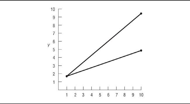
Be careful when testing differences in correlation coefficients, however, because a lack of difference in correlation coefficients does not necessarily mean that the relationship between the variables is the same. This problem is illustrated in Table 11.3. The correlation between Variable X and Variable Y is r = .98 for each group, indicating that one could predict Y scores equally well from X scores in both groups. However, as shown in Figure 11.4, scores on Y increase twice as fast for each increment in X in Group 2 (slope = .97) than they do in Group 1 (slope = .48). For example, if Y represented salary and X represented years of experience, with Group 1 being women and Group 2 being men, then the salary difference between men and women increases as experience increases: Although men and women start at the same salary, men’s salaries increase faster than women’s (the slopes are different). Nonetheless, men’s and women’s salaries can be predicted from years of experience with equal accuracy using the within-groups regression equation (the correlations are the same).
The apparent contradiction between the conclusions drawn from r and slope arises because r is a standardized index: X and Y scores are transformed to have a mean of 0 and a standard deviation of 1. Slope, in contrast, is an unstandardized index based on the raw (unstandardized) standard deviations of X and Y. Slope and r are related through the standard deviations (sd) of X and Y: b = r (sdx / sdy). For the data in Table 11.3, the standard deviation of Y is larger in Group 2 (2.98) than in Group 1 (1.49), whereas the standard deviation of X is constant for the two groups. Consequently, the value of b in Group 2 is twice that in Group 1. It is also possible for r to be different in two groups, but for b to have the same value in both groups. Therefore, whenever you compare correlations between two groups, check to ensure that their standard deviations are similar. If they are, there is no problem. If they are different, calculate the regression equations for each group and test the equality of slopes (see Cohen et al., 2003, for the formula). A difference in the slopes for a relationship in two groups represents an interaction between the grouping variable and variable X: The relationship between X and Y differs in the two groups. The results of the study should be interpreted accordingly: Because the relationship between the variables is different in the two groups, the grouping variable moderates their relationship.
Hypothetical Data Illustrating Equal Correlation but Different Slopes
X |
Y |
|
|
Group 1 |
Group 2 |
1 |
1 |
1 |
2 |
1 |
1 |
3 |
2 |
3 |
4 |
2 |
3 |
5 |
3 |
5 |
6 |
3 |
5 |
7 |
4 |
7 |
8 |
4 |
7 |
9 |
5 |
9 |
10 |
5 |
9 |
Plot of Regression Lines for the Data in Table 11.3.
As noted in Chapter 9, researchers often encounter the problem of an extraneous variable—a variable other than the independent variable that affects the dependent variable—which must be controlled. In an experiment, this control can be achieved through holding the variable constant, matched random assignment of research participants to conditions, or blocking on the extraneous variable. In correlational research, researchers cannot assign people to conditions of the independent variable because they are dealing solely with measured variables. Therefore, when investigating the relationship between one variable, X, and another, Y, there may be some extraneous third variable, Z, that is correlated with both X and Y, raising the question of what the correlation of X with Y would be if Z were not also correlated with them.
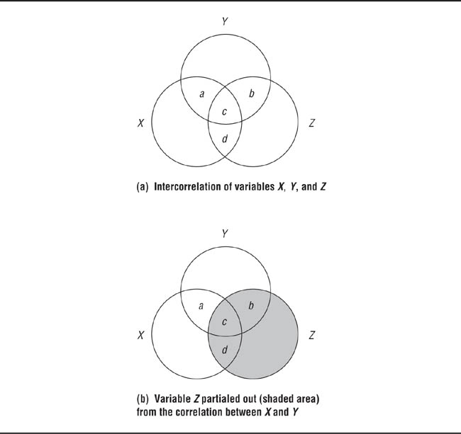
This problem is illustrated in Figure 11.5, in which variables are represented by circles and correlations are represented by overlapping areas of the circles. In panel (a), the correlation of X with Y is represented by Area a + c, the correlation of Z with Y by Area b + c, and the correlation of X with Z by Area c + d. The research question is “What would be the correlation of X with Y if Z were not there?” By removing the circle representing Z from the diagram as shown in panel (b) of Figure 11.5, the answer is seen to be Area a. This process controls for the effects of Z because the resulting partial correlation shows what the relationship between X and Y would be if all the research participants had the same score on Z, just as random assignment of participants to conditions in an experiment assumes that group means on extraneous variables are equal.
Correlations Among Three Variables.
The correlation between X and Y with Z controlled is represented by area a.
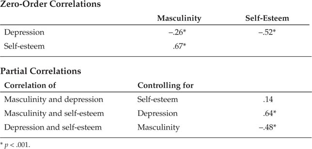
The partial correlation coefficient (pr) is interpreted in the same way as the simple (or zero-order) correlation coefficient, r: Just as r represents the strength of the relationship between two variables, pr represents the strength of that relationship when the effect of a third variable is removed or held constant. As illustrated in Figure 11.5, pr (Area a) will usually be smaller than r (Area a + c). As an example of partial correlation analysis, consider a study by Feather (1985). Feather noted that positive correlations are frequently found between self-esteem and a personality characteristic called psychological masculinity, and that negative correlations are frequently found between masculinity and depression. However, he went on to note, self-esteem is also negatively correlated with depression. Because some theories hold that masculinity should be related to depression independently of other factors, Feather investigated the question of what the correlation between masculinity and depression would be if self-esteem were controlled; that is, what is the partial correlation of masculinity with depression controlling for self-esteem? Table 11.4 shows the results of Feather’s study. The correlation between masculinity and depression controlling for self-esteem was substantially reduced from its zero-order level. However, the correlation between self-esteem and depression controlling for masculinity was essentially unchanged. Feather therefore concluded that the relationship between masculinity and depression could be almost completely accounted for by masculinity’s correlation with self-esteem. That is, he concluded that the masculinity-depression relationship was spurious, or false, because masculinity and self-esteem were confounded—the real relationship was between self-esteem and depression.
Results of Feather’s (1985) Study
The correlation between masculinity and depression becomes nonsignificant when self-esteem is controlled, but the correlation between self-esteem and depression is virtually unaffected when masculinity is controlled.
Multiple regression analysis (MRA) is an extension of simple and partial correlation to situations in which there are more than two independent variables. MRA can be used for two purposes. The first purpose is to derive an equation that predicts scores on some criterion (dependent) variable from a set of predictor (independent) variables. For example, the equation Y = a + b 1X1 + b2X2 estimates the value of a variable, Y, from two predictors, X1and X2; a is the intercept, as in bivariate regression, and b1 and b2 are the weights given to variables X1 and X2, respectively. The Schuman et al. (1985) study cited earlier used MRA to determine the degree to which college GPA could be predicted from three variables: SAT scores, hours of study, and class attendance. Their prediction equation could be written as Y = 1.99 + .0003X1 + .009X2 +.008X3, where Y represents GPA, X1 represents SAT score, X2 represents hours of study, and X3 represents class attendance. Therefore, a student with a combined SAT score of 1,000 who spent 2 hours a day studying and attended 90% of all class meetings could expect a GPA of 3.03.
MRA can also be used to explain variation in a dependent variable in terms of its degree of association with members of a set of measured independent variables, similar to the way in which factorial analysis of variance explains variation in a dependent variable in terms of the effect caused by a set of manipulated independent variables. However, because MRA is carried out through a series of partial correlation analyses, MRA, in contrast to analysis of variance, does not assume that the independent variables are uncorrelated.
This section examines a number of issues involved in the use of MRA. It begins with a look at the ways in which MRA can be conducted and the information that MRA can provide. Then, multicollinearity, a major potential threat to the validity of MRA, is discussed. Finally, two situations are examined in which MRA might be preferred to analysis of variance as a means of data analysis.
MRA can take three forms—simultaneous, hierarchical, and stepwise. Of these, only simultaneous and hierarchical analysis should be used because the results of stepwise regression can be misleading (see Thompson, 1995, for an overview of the issues involved). Consequently, this discussion covers only simultaneous and hierarchical analysis.
Simultaneous MRA. The purpose of simultaneous MRA is to derive the equation that most accurately predicts a criterion variable from a set of predictor variables, using all the predictors in the set. Note that simultaneous MRA is not designed to determine which predictor does the best job of predicting the criterion, which is second best, and so forth, but only to derive the best predictive equation using an entire set of predictors. For example, one might use a number of variables—such as SAT scores, high school GPA, and so forth—to try to predict college GPA. When the predictor variables are relatively uncorrelated with one another, the use of multiple predictors will lead to greater predictive accuracy than does the use of any one of the predictors by itself. This increase in the predictive utility of the regression equation occurs because most criterion variables have multiple predictors, and the more predictors that are used in estimating the criterion, the more accurate the estimation will be.
Hierarchical MRA. Hierarchical MRA is similar to partial correlation analysis. In the example given earlier, Feather (1985) asked the question of whether there a relationship between masculinity and depression after self-esteem is partialed out. In this case, he chose to partial self-esteem in order to answer his research question. Although Feather partialed only one variable (self-esteem) before considering the relationship between masculinity and depression, hierarchical MRA allows as many variables to be partialed as the investigator needs, in the order he or she wants to use. The researcher therefore creates the regression equation by adding, or entering, variables to the equation. This control by the investigator over the order of partialing makes hierarchical MRA appropriate for testing hypotheses about relationships between predictor variables and a criterion variable with other variables controlled.
Whitley’s (1990b) study on the relationship of people’s beliefs about the causes of homosexuality to their attitudes toward lesbians and gay men provides an example of the use of hierarchical MRA to test a hypothesis. Drawing on attribution theory (Weiner, 1986), which deals with how one’s interpretations of the causes of other people’s actions affect one’s reactions to those people, Whitley hypothesized that the greater the degree to which people perceived the causes of homosexuality to be under a person’s control, the more negative their attitudes toward lesbians and gay men would be. Whitley also collected data on two sets of extraneous variables. First, prior research indicated that attitudes toward gay people were related to at least three other variables (Herek, 1988): the sex of the research participant, whether the gay person was of the same sex as the research participant, and whether the participant knew a lesbian or a gay man. Second, attribution theory also includes two constructs in addition to controllability that are not supposed to be related to attitudes: the extent to which a cause is perceived to be a function of the person rather than of the environment (internality) and the perceived stability of the cause over time. The research question therefore was whether controllability attributions were related to attitudes toward lesbians and gay men with the effects of the other variables controlled.
The results of the MRA are shown in Table 11.5. Consistent with previous research, sex of the gay person toward whom participants were expressing their attitudes, similarity of sex of participant and gay person, and acquaintance with a lesbian or gay man were all related to attitudes toward gay people. In addition, controllability attributions were significantly related to these attitudes, but the other attributions were not. Whitley (1990b) therefore concluded that controllability attributions were related to attitudes toward lesbians and gay men even when other important variables were controlled.
MRA can provide three types of information about the relationship between the independent variables and the dependent variable: the multiple correlation coefficient, the regression coefficient, and the change in the squared multiple regression coefficient. Each of these statistics can be tested to determine if its value is different from zero.
TABLE 11.5
Results of Whitley’s (1990b) Study
As hypothesized, controllability attributions had a significant relationship to attitudes toward lesbians and gay men with the other variables controlled.
Variable |
ß |
Sex of respondent (R)a |
-.082 |
Sex of target person (T)a |
-.126* |
Similarity of R and Tb |
-.318** |
Acquaintance with gay person |
.276** |
Stability attribution |
-.002 |
Internality attribution |
-.066 |
Controllability attribution |
-.201** |
Note: |
A higher attitudes score indicates a more favorable attitude. ß is an index of the strength of the relationship (see next section) |
aScored female = 1, male = 2
bScored same = 1, different = 2
*p .05. **p .001.
The multiple correlation coefficient. The multiple correlation coefficient (R) is an index of the degree of association between the predictor variables as a set and the criterion variable, just as r is an index of the degree of association between a single predictor variable and a criterion variable. Note that R provides no information about the relationship of any one predictor variable to the criterion variable. The squared multiple correlation coefficient (R2) represents the proportion of variance in the criterion variable accounted for by its relationship with the total set of predictor variables. For a given set of variables R2 will always be the same regardless of the form of MRA used.
The regression coefficient. The regression coefficient is the value by which the score on a predictor variable is multiplied to predict the score on the criterion variable. That is, in the predictive equation Y = a + bX, b is the regression coefficient, representing the slope of the relationship between X and Y. Regression coefficients can be either standardized (β, the Greek letter beta) or unstandardized (B). In either case, the coefficient represents the amount of change in Y brought about by a unit change in X. For β, the units are standard deviations, and for B, the units are the natural units of X, such as dollars or IQ scores. Because the βs for all the independent variables in an analysis are on the same scale (a mean of 0 and a standard deviation of 1), researchers can use these coefficients to compare the degree to which the different independent variables used in the same regression analysis are predictive of the dependent variable. That is, an independent variable with a β of .679 better predicts (has a larger partial correlation with) the dependent variable than an independent variable with a β of .152, even though both may be statistically significant. In contrast, because the Bs have the same units regardless of the sample, these coefficients can be used to compare the predictive utility of independent variables across samples, such as for women compared to men. The statistical significance of the difference between the Bs for the same variable in two samples can be determined using a form of the t-test (Cohen et al., 2003).
Change in R2. Change in R2 is used in hierarchical MRA and represents the increase in the proportion of variance in the dependent variable that is accounted for by adding another independent variable to the regression equation. That is, it addresses the question of whether adding X2 to the equation helps to predict Y any better than does X1 alone. Change in R2 is a ratio level variable; that is, it is legitimate to state that an independent variable that results in a change in R2 of .262 predicts twice as much variance in the dependent variable than one that results in a change in R2 of .131.
However, the change in R2 associated with an independent variable can fluctuate as a function of the order in which the variable is entered into the equation. Entering a variable earlier will generally result in a larger change in R2 than entering it later, especially if it has a high correlation with the other predictor variables. Consider, for example, the situation shown in Table 11.6. The zero-order correlations represent graduate students’ scores on a measure of motivation to succeed in graduate school, ratings of the qualifications for admission to graduate school, their graduate school GPAs, and their scores on their predoctoral comprehensive examination. The second part of the table shows the change in R2 for motivation predicting exam scores when it is entered in the regression equation in different orders. As you can see, the change in R2 ranges from .258 to .018 depending on the order of entry. It is therefore essential to think carefully about the order in which you enter variables in MRA.
Multicollinearity is a condition that arises when two or more predictor variables are highly correlated with each other. Multicollinearity can have several adverse effects on the results of MRA, so researchers must be aware of the problem, check to see if it is affecting their data, and take steps to deal with it if it is found.
Effects of multicollinearity. One effect of multicollinearity is inflation of the standard errors of regression coefficients. Artificially large standard errors can lead to a nonsignificant statistical test and the erroneous conclusion that there is no relationship between the predictor variables and the criterion variable. Multicollinearity can also lead to misleading conclusions about changes in R2. If two predictor variables are highly correlated, when the relationship of one predictor variable is partialed out from the criterion variable, the second predictor variable is left with only a small partial correlation with the criterion variable. For these reasons, multicollinearity poses a grave threat to the validity of conclusions drawn from MRA.
Causes of multicollinearity. Multicollinearity can arise from several causes. One cause is the inclusion of multiple measures of one construct in the set of predictor variables. Because measures of the same construct will be highly correlated, they will lead to multicollinearity. If multiple measures of constructs are to be used—generally a good practice—a latent variables approach (described in the next chapter) should be taken to the data analysis. Some variables, such as height and weight, are naturally correlated and so can lead to multicollinearity. In other cases, measures of conceptually different constructs have highly correlated scores; scores on depression and anxiety measures, for example, are often highly correlated (Dobson, 1985). Finally, sampling error can lead to artificially high correlations between variables in a data set: Two variables with a moderate correlation in the population might be highly correlated in a sample because people who scored high on both variables or low on both variables were accidentally oversampled relative to their incidence in the population. For example, sex and IQ scores are uncorrelated in the population, but a sample might contain an unrepresentatively high number of high-scoring women and low-scoring men, thereby producing a correlation between sex and IQ score in the sample.
Detecting multicollinearity. Because of its adverse effects, it is very important to test the correlation matrix of predictor variables for multicollinearity before conducting MRA. Statisticians have developed a number of guidelines for detecting the presence of multicollinearity (see, for example, Cohen et al., 2003); unfortunately, because multicollinearity is a characteristic of a sample rather than of a population, there is no statistical test for it. The simplest way to assess multicollinearity is by inspecting the correlation matrix; correlations equal to or greater than .80 are generally taken as being indicative of multicollinearity (Licht, 1995). Inspection, however, can determine only if there is a high correlation between two variables; multicollinearity is also a function of the pattern of correlations among several predictors, none of which might exceed .80, so multicollinearity might not be detectable through inspection. A mathematical indicator of multicollinearity that is provided by most statistical software packages is the variance inflation factor (VIF). Generally, a VIF of 10 or greater is considered to be indicative of multicollinearity (Cohen et al., 2003).
Dealing with multicollinearity. One solution to the problem of multicollinearity is preventive: Avoid including redundant variables, such as multiple measures of a construct and natural confounds, in the set of predictor variables. Instead, combine them into indexes, such as the mean standard score on a set of depression measures or a weight-height ratio. If some measures of conceptually different constructs tend to be highly correlated, use the measures that show the least correlation. If multicollinearity is still present after these steps have been taken, you can try other solutions. If sampling error could be the source of an artificial confound, collecting more data to reduce the sampling error might reduce the problem. Another solution is to delete independent variables that might be the cause of the problem. In that case, however, you might also be deleting valuable information. Finally, you might conduct a factor analysis (described in the next chapter) to empirically determine which variables to combine into an index. However, the theoretical or practical meaning of a variable constructed in this way and the meaning of its relationship to the dependent variable might be unclear.
As we noted earlier, correlational analyses assume that the relationships of the independent variables to the dependent variable are linear and additive. That is, the use of correlational analyses assumes there are no curvilinear relationships between the independent and dependent variables and no interactions among the independent variables. There are, however, mathematical ways around these assumptions. The arithmetic-square of the score on an independent variable can be used to represent the curvilinear effect of the variable; that is, you can use a variable that is equal to X2 to represent the curvilinear effect of X. The arithmetic product of the scores for two independent variables can be used to represent their interaction; for example, you can create a variable that is equal to X times Z to represent the interaction of X and Z. However, MRA using nonlinear and interaction terms must be carried out very carefully to avoid inducing multicollinearity and its associated problems. See Cohen et al. (2003) for more information about these kinds of analyses. One implication of this ability to include nonlinear and interaction terms in MRA is that you can use it in place of a factorial ANOVA. There are two conditions when MRA would be preferred to ANOVA: when one or more of the independent variables is measured on a continuous scale, and when independent variables are correlated.
Continuous independent variables. In ANOVA, when an independent variable is measured as a continuous variable, such as a personality trait, it must be transformed into a categorical variable so that research participants can be placed into the discrete groups required by ANOVA. This transformation is often accomplished using a median split: the median score for the sample being used is determined, with people scoring above the median being classified as “high” on the variable and those scoring below the median being classified as “low.” This procedure raises conceptual, empirical, and statistical problems. The conceptual problem is illustrated in Figure 11.6, which presents the scores of four research participants—A, B, C, and D—on a continuous variable. As you can see, use of a median split to classify participants on this scale makes the implicit assumptions that Participant A is very similar to Participant B, that Participant C is very similar to Participant D, and that Participants B and C are very different from each other. The problem is whether these assumptions are tenable for the hypothesis being tested; often they will not be.
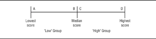
Use of Median Split to Classify Research Participants into Groups on a Continuous Variable.
The empirical problem brought about by the use of median splits is that of the reliability of the resulting classification of research participants. Because classification cutoff scores are relative (changing from sample to sample as the median changes) rather than absolute, participants who are in different samples but who have the same scores might be classified differently. This problem is especially likely to occur in small samples, in which the sample median might be a poor estimate of the population median. Comparability of results across studies is therefore reduced. Comparability can be further reduced when different studies use median splits on different measures of the same construct. For example, although scores on Bem’s (1974) Sex Role Inventory and Spence, Helmreich, and Stapp’s (1975) Personal Attributes Questionnaire (two measures of the personality variable of sex role self-concept) are highly correlated, agreement between category classification based on median splits is only about 60%, which is reduced to about 40% when agreements due to chance are taken into account (Kelly, Furman, & Young, 1978).
Median splits engender two statistical problems. The first is that of power—the ability of a sample correlation to accurately estimate the population correlation. Bollen and Barb (1981) have shown that given a population correlation of r = .30—the conventionally accepted level of a moderate correlation (Cohen, 1992)—the estimated r in large samples is .303, whereas using a median split gives an estimate of r = .190, much smaller than the true size of the correlation. Although increasing the number of categories improves the sample correlation relative to its population value (for example, three categories gave an estimate of r = .226 in Bollen and Barb’s study), there is always some loss of power. The second statistical problem is that the use of median splits with two or more correlated independent variables in a factorial design can lead to false statistical significance: A main effect or interaction appears statistically significant when, in fact, it is not (Maxwell & Delaney, 1993). This outcome can occur because dichotomizing two correlated independent variables confounds their effects on a dependent variable so that in an ANOVA the “effect” for one independent variable represents not only its true relationship with the dependent variable but also some of the other independent variable’s relationship with the dependent variable. Consequently, the apparent effect of the first independent variable is inflated. The more highly correlated the predictor variables, the more likely false significant effects become.
These problems all have the same solution: Treat the independent variable as continuous rather than as a set of categories and analyze the data using MRA. One might argue, however, that sometimes a researcher wants to investigate both an experimentally manipulated (thus, categorical) variable and a continuous variable in one study. For example, Rosenblatt and Greenberg (1988) investigated the relationships of research participants’ level of depression (a personality variable) and the characteristics of another person (a manipulated variable) to the participants’ liking for the person. Because the manipulated variable in such studies is categorical, one might think it necessary to categorize the personality variable and use ANOVA to analyze the data. However, MRA can accommodate categorical variables such as the conditions of an experiment as well as continuous variables by assigning values, such as 1 and 0, to the experimental and control conditions of the manipulated variable. The situation becomes more complex if the manipulated variable has more than two conditions; see Cohen et al. (2003) for information on how to handle such situations.
Correlated independent variables. Because ANOVA assumes that the independent variables are uncorrelated and MRA does not, the second condition under which MRA is to be preferred to ANOVA is when independent variables are correlated. Correlations between categorical independent variables can occur when there are unequal numbers of subjects in each group. The 2-to-1 female-to-male ratio in psychiatric diagnoses of depression (Nolen-Hoeksema, 1987), for example, means that gender and receiving a diagnosis of depression are correlated. If these variables were to be used as factors in an ANOVA, the assumption of uncorrelated independent variables would be violated and the validity of the analysis could be open to question. Therefore, if you conduct a factorial study with unequal group sizes, test to see if the factors are correlated. If they are, use MRA rather than ANOVA.
Simple and partial correlation analysis and MRA are probably the most commonly used correlational techniques. However, all three approaches assume that the dependent variable in the research is continuous, although some forms of the correlation coefficient, such as the point biserial correlation, can be used when one of the variables is dichotomous. This section briefly looks at two correlational techniques designed for categorical dependent variables—logistic regression analysis and multiway frequency analysis—and concludes with a note on the relation between data types and data analysis.
MRA uses a set of continuous independent variables to predict scores on a continuous dependent variable. What is to be done if the dependent variable is categorical? The answer to this question is a technique called logistic regression analysis. Logistic regression analysis can be used for most of the same purposes as MRA, but in some ways it is a more flexible tool for data analysis (Tabachnick & Fidell, 2007). For example, unlike MRA, logistic regression does not assume that variables have normal distributions or that the relationships between the independent and dependent variables are linear. However, because the criterion variable is categorical rather than continuous, interpretation of the results is more complex. To give one example, unlike the regression coefficient, the odds ratio (OR) used in logistic regression does not represent the amount of change in the dependent variable associated with a unit change in the independent variable; it describes the likelihood that a research participant is a member of one category of the dependent variable rather than a member of the other categories. An OR of 1 for a variable indicates that scores on it are unrelated to membership in the dependent variable categories. An OR greater than 1 indicates that higher scoring participants are more likely to be in a target group (such as high smokers); an OR less than one means that higher scores are more likely to be in the other group.
Selected Results from Griffin, Botvin, Doyle, Diaz, and Epstein’s (1999) Study of Predictors of Adolescent Smoking
|
Odds Ratios | ||
|
Girls |
Boys | |
Father smokes |
2.16 |
1.38 | |
Mother smokes |
2.29* |
2.01* | |
One sibling smokes |
3.52** |
0.85 | |
More than half of friends smoke |
3.14** |
8.23*** | |
Parents are not opposed to smoking |
3.55* |
0.95 | |
Friends are not opposed to smoking |
10.50*** |
1.21 | |
Hold anti-smoking attitudes |
0.48** |
0.37 | |
*p .05. **p .01. ***p .001.
For example, Griffin, Botvin, Doyle, Diaz, and Epstein (1999) used logistic regression to investigate factors that predict adolescent cigarette smoking. They used scores on variables measured when the research participants were in seventh grade to predict which participants would be heavy smokers in the 12th grade. Table 11.7 shows some of Griffin et al.’s findings. Compared to nonsmokers and light smokers, girls who were heavy smokers were 2.29 times as likely to have a mother who smoked, 3.52 times as likely to have a sibling who smokes, 8.14 times as likely to have parents who were not opposed to smoking, 10.5 times as likely to have friends who were not opposed to smoking, and about half as likely to hold anti-smoking attitudes. For boys, only having a mother who smoked and a large number of friends who smoked were related to heavy smoking.
Multiway frequency analysis allows a researcher to examine the pattern of relationships among a set of nominal level variables. The most familiar example of multiway frequency analysis is the chi-square (X2) test for association, which examines the degree of relationship between two nominal level variables. For example, one theory of self-concept holds that people tend to define themselves in terms of characteristics that set them apart from most other people with whom they associate (McGuire & McGuire, 1982). Kite (1992) tested this proposition in the college context, hypothesizing that “nontraditional” college students, being older than most college students, would be more likely to define themselves in terms of age than would college students in the traditional age range or faculty members who, although older than traditional college students, are in the same age range as the majority of their peers. Research participants were asked to write a paragraph in response to the instruction to “Tell us about yourself”; the dependent variable was whether the participants referred to their ages in their responses. Table 11.8 shows the distribution of responses: “Nontraditional” students were more likely to mention their ages than were members of the other groups.
Loglinear analysis extends the principles of chi-square analysis to situations in which there are more than two variables. For example, Tabachnick and Fidell (2007) analyzed data from a survey that asked psychotherapists about being sexually attracted to clients (Pope, Keith-Spiegel, & Tabachnick, 1986). Tabachnick and Fidell examined the relationships among five dichotomous variables: whether the therapist thought that the client was aware of the therapist’s being attracted to him or her, whether the therapist thought that the attraction was beneficial to therapy, whether the therapist thought that it was harmful to therapy, whether the therapist had sought the advice of another professional about being sexually attracted to a client, and whether the therapist felt uncomfortable about being sexually attracted to a client. Tabachnick and Fidell found that 58% of the therapists who had felt attracted to a client had sought advice (the researchers used the term consultation) about the attraction. Seeking advice was also related to other variables in the study:
Two-Way (3 x 2) Frequency Table showing Percentages of people in Three Categories Who Did or Did Not Mention Their Ages When Describing Themselves
|
Group |
||
|
Traditional Students |
“Nontraditional” Students |
Faculty Members |
Mention of age |
16.3% |
57.1% |
35.7% |
No mention of age |
83.7% |
42.9% |
64.3% |
Note: Adapted from Kite, 1992, p. 1830.
Those who sought consultation were … more likely to see the attraction as beneficial. Of those seeking consultation, 78% judged the attraction to be beneficial. Of those not seeking consultation, 53% judged it beneficial.… Seeking consultation was also related to client awareness and therapist discomfort. Therapists who thought clients were aware of the attraction were more likely to seek consultation (80%) than those who thought the client unaware (43%). Those who felt discomfort were more likely to seek consultation (69%) than those who felt no such discomfort (39%). (Tabachnick & Fidell, 2007, pp. 907–908)
When one of the variables in a loglinear analysis is considered to be the dependent variable and the others are considered to be independent variables, the procedure is sometimes called logit analysis. Logit analysis is analogous to ANOVA for nominal level dependent variables, allowing the assessment of main effects and interactions for the independent variables. For example, Epperson, Bushway, and Warman (1983) conducted a study to examine the relationship of three counselor variables to their clients’ propensity to drop out of counseling after only one session. The variables were sex of counselor, counselor’s experience level (trainee or staff counselor), and whether or not the counselor accepted clients’ definitions of their problems, a variable that Epperson et al. called problem recognition. Epperson et al. found two main effects: female counselors had higher client dropout rates (33%) than did male counselors (20%), and counselors who did not accept clients’ problem definitions had higher dropout rates (55%) than counselors who did accept clients’ problem definitions (19%). Epperson et al. also found an interaction between counselor experience and problem recognition: Trainees had similar client dropout rates regardless of whether they accepted clients’ problem definitions (27%) or not (32%), whereas experienced counselors who did not accept clients’ problem definitions had a much higher dropout rate (59%) than those who did (17%).
|
Independent Vatiable | |
Dependent Variable |
Categorical |
Continuous |
Categorical |
Chi-square analysis |
Logistic regression analysis |
|
Loglinear analysis |
|
|
Logit analysisa |
|
Continuous |
Analysis of variance |
Multiple regression analysis |
a |
If the distribution of scores on the dependent variable meets certain requirements, dichotomous dependent variables can be analyzed by ANOVA or the t-test. See Lunney, 1970, and Myers, DiCecco, White, & Borden, 1982. |
Let’s conclude our discussion of correlational research by tying together a set of concepts from this chapter and the previous chapter. Think of variables as providing two types of data—categorical (nominal level) and continuous (interval and ratio level)—and as being either the independent or dependent variables in a study. The two types of data and two roles for variables result in the four combinations shown in Table 11.9. Each combination of categorical or continuous independent variable and categorical or continuous dependent variable has an appropriate statistical procedure for data analysis. Be sure to use the right form of statistical analysis for the combination of data types that you have in your research.
Correlational research methods can be used to test hypotheses that are not amenable to experimental investigation, either because the constructs used as independent variables cannot be manipulated or because manipulation of the independent variables would be unethical. This chapter reviewed the nature of correlational research and the principal methods of correlational research.
Except for special forms of multiple regression analysis, correlational research methods assume that the relationship between the independent and dependent variables are linear and additive. A number of factors can have adverse effects on the sizes of correlation coefficients. The reliability of measures puts a ceiling on the size of the correlation between their scores, and restriction in the range of scores attenuates the correlation. Outliers can either artificially inflate or deflate the correlation depending on their relation to the bulk of the scores. Differences in subgroups in the participant sample can result in a correlation for the entire sample that misrepresents the relationship between the variables in the subgroups. When conducting research with multifaceted constructs, one should generally treat the facets of the construct as separate variables rather than combine them into a general index of the construct. Using a general index can obscure the unique relationships of the facets to the dependent variable and make it impossible to detect interactions among the facets.
Although simple correlation is the basis for all correlational research, most studies use more complex techniques. A difference in the slope of the relationship between two variables in different groups represents an interaction between the grouping variable and the variables being tested. Partial correlation determines the relationship between two variables when the effects of a third variable are controlled.
Multiple regression analysis (MRA) examines the relationships among the members of a set of predictor variables to a criterion variable. Simultaneous MRA provides an equation that most accurately predicts the criterion variable using all the predictor variables. Hierarchical MRA allows the researcher to partial out multiple predictors from the relationship between another predictor and the criterion. Because it controls the effects of the partialed predictors, hierarchical MRA is best suited for hypothesis testing. Stepwise MRA has a number of statistical flaws and should not be used. MRA provides three types of information on the relationship between the predictor variables and the criterion variable. The multiple correlation coefficient (R) is an index of the size of the relationship between the predictor variables as a set and the criterion. A predictor’s regression coefficient is an index of the size of its relationship with the criterion. Change in R2 indicates the amount of variance in the criterion that is accounted for by adding a predictor variable to hierarchical regression. Multicollinearity is a potential problem in MRA that stems from high correlations among the predictor variables. Multicollinearity can result from having multiple measures of a construct in the set of predictor variables, from natural confounds, or from sampling error, and it can be overcome by deleting redundant variables from the predictor set or by combining multicollinear predictors into a single variable. MRA is useful as an alternative to ANOVA when the independent variables are correlated or when the independent variables are continuous rather than categorical. Although continuous variables can be transformed into categories, this procedure can have an adverse impact on the research.
Logistic regression analysis is analogous to MRA but is used with a nominal level (categorical) dependent variable. It also incorporates fewer statistical assumptions than does MRA. Multiway frequency analysis can be used when both the independent and dependent variables are measured at the nominal level. Types of multiway frequency analysis include chi-square analysis, loglinear analysis, and logit analysis.
Cohen, J., Cohen, P., West, S. G., & Aiken, L. S. (2003).Applied multiple regression/correlation analysis for the behavioral sciences (3rd ed.). Mahwah, NJ: Erlbaum.
Grimm, L. G., & Yarnold, P. R. (Eds.). (1995).Reading and understanding multivariate statistics. Washington, DC: American Psychological Association.
Tabachnick, B. G., & Fidell, L. S. (2007). Using multivariate statistics (5th ed.). Boston, MA: Pearson.
Chapters 2 and 7 in Grimm and Yarnold’s book provide excellent nontechnical introductions to multiple regression analysis and logistic regression analysis. Tabachnick and Fidell cover these topics (plus multiway frequency analysis) in more technical detail and also provide examples of how to carry out these analyses using two statistical packages, SAS and SPSS (now PAWS). Cohen et al. provide a detailed analysis of the issues involved in conducting and interpreting the results of multiple regression analyses, including analyses the incorporate nonlinear and interaction effects.
Marsh, H, W., Dowson, M., Pietsch, J., & Walker, R. (2004). Why multicollinearity matters: A reexamination of relations between self-efficacy, self-concept, and achievement. Journal of Educational Psychology, 96(3), 518–522.
Marsh and colleagues provide an example of the ways in which multicollinearity can lead to incorrect interpretation of the results of research.
Additivity
Attenuation
Bivariate regression
Change in R2
Criterion variable
Curvilinear relationship
Hierarchical multiple regression analysis
Intercept
Latent variable
Linearity
Logistic regression analysis
Logit analysis
Loglinear analysis
Median split
Multicollinearity
Multiple correlation coefficient
Multiple regression analysis
Multiway frequency analysis
Outlier
Partial correlation
Predictor variable
Regression coefficient
Restriction in range
Simultaneous multiple regression analysis
Slope
Zero-order correlation
1. |
Describe the circumstances in which the correlational research strategy would be preferable to the experimental strategy. What can correlational research tell us about causality? |
2. |
Describe the effects of each of these factors on the size of the correlation coeffi cient: |
a. |
Low reliability of the measures |
b. |
Restriction in range |
c. |
Outliers |
Subgroup differences in the correlation between the variables |
4. |
For the factors listed in Question 2, describe how you can determine if a problem exists and describe what can be done to rectify the problem. |
5. |
Find three recent journal articles on a topic that interests you that used correlational research. Did the researchers report whether they checked for the potential problems listed in Question 2? If they found any, did they take the appropriate steps? If they did not check, how would the presence of each potential problem affect the interpretation of their results? |
6. |
If you find a significant difference between groups, such as men and women, in the size of the correlation between two variables, how should you interpret the finding? |
7. |
Explain why it is generally undesirable to combine the facets of a multifaceted construct into an overall index. Describe the circumstances under which it might be useful to combine facets. |
8. |
Describe the purpose of partial correlation. |
9. |
Describe the forms of multiple regression analysis (MRA) and the purpose for which each is best suited. |
a. |
Describe the type of information that each of the following provide about the relationship between the predictor variables and the criterion variable in MRA: |
b. |
The multiple correlation coefficient (R) |
c. |
The standardized regression coefficient (β) |
d. |
The unstandardized regression coefficient (B) d Change in R2 |
10. |
What is multicollinearity? Describe its effects. How can you detect and deal with this problem? |
11. |
Describe the circumstances under which MRA is preferable to ANOVA. |
12. |
What is a median split? Why is it undesirable to use a median split to transform a continuous variable into a categorical variable? |
13. |
How is logistic regression analysis similar to MRA and how is it different? |
14. |
When should a researcher use multiway frequency analysis? |
15. |
How does the nature of the independent and dependent variables affect the form of data analysis you should use? |