Principles of Research in Behavioral Science

In Chapter 11 we described some of the basics of correlational research; in this chapter we examine some extensions of those basic methods. The first topic we address is factor analysis, a set of techniques for determining the extent to which a set of variables represents a single underlying hypothetical construct. Exploratory factor analysis starts with a set of variables and searches for relationships among them; confirmatory factor analysis starts with a hypothesis about the pattern of relationships among a set of variables and tests that hypothesis. We then provide an overview of methods for testing mediational hypotheses. Mediational hypotheses (or models) propose that one or more variables come between an independent variable and a dependent variable in a causal sequence. For example, Event → Interpretation of event → Response to event represents a mediational model in which the way in which a person interprets an event (as, say, threatening versus nonthreatening) affects how the person responds to the event.

The overviews we present here are very brief and are intended to give you a framework to use when reading journal articles and other publications that utilize these methods. This chapter may also give you ideas for your own research. However, the application of these methods to data you collect entails many issues and complexities that we do not address here; you should take a class on these methods and consult a statistical expert before using them yourself.

Exploratory Factor Analysis

The term factor analysis refers to a set of statistical techniques used to examine the relationships among a set of intercorrelated variables, such as responses to items on a measure of a hypothetical construct. In using factor analysis one assumes that the variables are intercorrelated because they reflect one or more underlying dimensions or factors. For example, responses to items on a measure are assumed to be correlated with one another because each item reflects an aspect of the construct being measured, as illustrated in Figure 12.1. In the figure, the circle represents the hypothetical construct (which cannot be directly observed) and the rectangles represent responses to the items on the measure (which are directly observed). Arrows go from the construct to the items because people’s responses to the items are assumed to be caused by their status on the construct, such as a high or low level of self-esteem. Another technique, principal components analysis, is very similar to exploratory factor analysis, differing primarily in some statistical assumptions, so our discussion will focus on the more commonly used exploratory factor analysis.

FIGURE 12.1

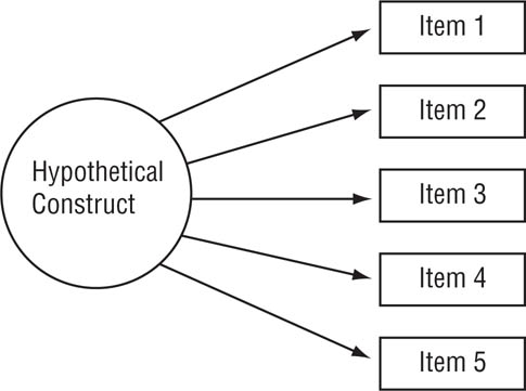
Relationship of Items on a Measure to the Hypothetical Construct Being Measured.

In an exploratory factor analysis, the five items should form a single factor because scores on the items are caused by a single underlying construct.

Box 12.1 Items for an Attitude toward Computer Scale


1.	I look forward to using a computer in my work.
2.	I’m afraid of computers.
3.	I feel more competent working with computers than do most people.
4.	I dislike computers.
5.	I could create a simple database on a computer.
6.	People are becoming slaves to computers.
7.	Soon our lives will be controlled by computers.
8.	I feel intimidated by computers.
9.	Computers are dehumanizing to society.
10.	Computers can eliminate a lot of tedious work for people.
11.	The use of computers is enhancing our standard of living.
12.	Computers are a fast and efficient means of gathering information.
13.	I avoid computers as much as possible.
14.	Computers will replace the need for working people.
15.	Computers are bringing us into a bright new era.
16.	Soon our world will be completely run by computers.
17.	Life is easier because of computers.
18.	I feel that having a computer would help me in my work.
19.	I prefer not to learn how to use a computer.
20.	I would like to own, or do own, a computer.

Source: Items adapted from Heinssen, Glass, and Knight (1987); Meier (1988); Nickell and Pinto (1986); and Popovich, Hyde, Zakrajsek, and Blummer (1987).

Exploratory factor analysis is a statistical technique that can be applied to a set of variables to identify subsets of those variables in which the variables in a subset are correlated with each other but are relatively uncorrelated with the variables in the other subsets. These subsets of variables are called factors. At a conceptual level, factors represent the processes that created the correlations among the variables. For example, a factor might represent a hypothetical construct, such as attitudes toward computers. Computer attitudes could be assessed by a set of items, such as those shown in Box 12.1. People who have similar attitudes toward computers should respond to the items in the same way, leading to correlations among the responses to the items. Exploratory factor analysis can examine the correlations among the responses to determine the extent to which responses to items are interrelated; the more strongly the item responses in a set are interrelated, the more likely it is that they represent one construct. If an exploratory factor analysis finds more than one factor in a set of variables, the factors might represent different constructs or different facets of a single multifaceted construct. For example, as we discuss later, the 20 items in Box 12.1, all of which deal with attitudes toward computers, represent four factors: feelings of anxiety related to using computers, perceived positive effects of computers on society, perceived negative effects of computers on society, and the personal usefulness of computers.

This section briefly examines the uses of exploratory factor analysis in research and the issues to consider when conducting or reading about exploratory factor analysis. For more detailed but still relatively nontechnical discussions of these issues, see Bryant and Yarnold (1995), Tabachnick and Fidell (2007), and Thompson (2004).

Uses of Exploratory Factor Analysis

At the most general level, exploratory factor analysis is used to summarize the pattern of correlations among a set of variables. For example, the 190 correlations among the scores on the 20 items in Box 12.1 can be summarized in terms of the four factors underlying those correlations. In practice, exploratory factor analysis can serve several purposes (Fabrigar, Wegener, MacCallum, & Strahan, 1999), two of which (data reduction and scale development) tend to predominate.

Data reduction. One use of exploratory factor analysis is to condense a large number of variables into a few variables to simplify data analysis. If you have a large number of correlated dependent variables in a study, it can be easier to understand the results if they are presented in terms of a few factors rather than many individual variables. Consider, for example, the question of whether there are sex differences in attitudes toward computers. You could administer a questionnaire composed of the items in Box 12.1 to men and women and test to see if there are sex differences in response to each item, but it could be difficult to draw overall conclusions from the results of 20 statistical tests. In contrast, it would be easier to draw conclusions from tests for sex differences on the four factors those items represent.

Scale development. The second major use of exploratory factor analysis is in the development of scales for measuring hypothetical constructs. As noted in Chapter 6, a scale should represent only one construct or be composed of subscales, each of which represents a construct or facet of a construct. After a set of items have been chosen for use on a scale, the scale developers administer the items to groups of people. The developers then use exploratory factor analysis to determine if responses to the items intercorrelate in the way they theoretically should. That is, exploratory factor analysis is one tool that can be used to examine the structural validity of a measure. For example, if a scale is supposed to measure just one construct, an exploratory factor analysis should find just one factor, which would represent that construct. If it finds more than one factor, the scale developers can discard the items that are not related to the factor that represents their construct. Similarly, if a scale is designed to measure more than one facet of a construct, there should be a factor for each facet.

Considerations in Exploratory Factor Analysis

Exploratory factor analysis is a very heterogeneous technique: There are multiple approaches to determining the number of factors underlying a set of correlations and multiple ways of simplifying those factors so that they can be easily interpreted (Tabachnick & Fidell, 2007). Consequently, there are a large number of opinions about the “right” way to conduct a factor analysis. The following discussion focuses on the more common questions that arise in factor analysis and on the most common answers to these questions. These points are illustrated with a factor analysis of responses to the 20 items shown in Box 12.1

Number of research participants. A major concern in exploratory factor analysis is the stability of the factors found—that is, the likelihood that a factor analysis of scores on the same items from another sample of people will produce the same results. One factor that influences stability is the number of respondents on which an exploratory factor analysis is based. There are no hard and fast rules for determining an adequate sample size, but most authorities recommend having at least 10 participants per item with a minimum of 200 to 300 participants (Tabachnick & Fidell, 2007). There were 314 respondents to the items in Box 12.1, which is an adequate sample size.

Quality of the data. The quality of the data also affects factor stability. Because exploratory factor analysis is based on correlations, all the factors noted in Chapter 11 as threats to the validity of correlational research—outliers, restriction in range, and so forth—also threaten the validity of a factor analysis. Multicollinearity is also a problem in factor analysis because a large number of extremely high correlations leads to problems in the mathematics underlying the technique.

The correlation matrix of the scores on the items to be factor analyzed should include at least several large correlations, indicating that sets of item responses are interrelated. Tabachnick and Fidell (2007) recommend not conducting an exploratory factor analysis if there are no correlations larger than .30. Because examining the correlations in a large matrix can be cumbersome, you can also examine the determinant of the correlation matrix, a statistic available in most factor analysis computer programs. The closer the determinant is to zero, the higher the correlations among the variables, and the more likely you are to find stable factors.

Examination of the distributions of scores for the sample factor analysis found no outliers. The correlation matrix contained many high correlations but did not exhibit multicollinearity. The determinant of the matrix was .0002. These results indicated that the matrix was highly “factorable.”

Factor extraction and rotation. The term extraction refers to the method used to determine the number of factors underlying a set of correlations. Factors are extracted in order of importance, which is defined as the percentage of variance in the variables being analyzed that a factor can account for. The first factor accounts for the most variance, the second factor for the next largest percentage of variance, and so forth. An exploratory factor analysis will initially extract as many factors as there are variables, each accounting for a decreasing percentage of variance. A number of extraction methods exist, but all give very similar results with high-quality data and a reasonable sample size (Tabachnick & Fidell, 2007).

The term rotation refers to the method used to clarify the factors once they are extracted. With unrotated factors it can be difficult to see which variables are associated with, or “load on,” which factor, because any variable can appear to be associated with more than one factor. Rotation minimizes these multiple loadings. There are two general categories of rotation. Orthogonal rotation forces factors to be uncorrelated with one another; oblique rotation allows factors to be correlated. There are several specific types of rotation in each category; however, like the different methods of extraction, different methods of rotation within the same category provide equivalent results with high-quality data and an adequate sample size (Tabachnick & Fidell, 2007). As a practical matter, Tabachnick and Fidell note that most researchers start an exploratory factor analysis with principal components extraction and varimax rotation (a type of orthogonal rotation) and move on to other methods based on the outcome of the initial analysis. For example, if the results of the initial analysis indicated that the factors might be correlated, the researchers could conduct another analysis using oblique rotation. However, other experts suggest starting with oblique rotation because if the factors are in fact uncorrelated, an oblique rotation will show that (Fabrigar et al., 1999). We used principle components analysis with varimax rotation for the example factor analysis because of the ease of interpreting the results provided by these methods.

Number of factors. In a perfect world, the results of an exploratory factor analysis would be able to tell you, “There are X number of factors underlying this correlation matrix, and that’s all.” Unfortunately, it’s not always easy to decide how many factors there “really” are underlying a set of correlations. The decision is as much a matter of judgment as statistics, so different researchers might have different interpretations of exploratory factor analyses of the same data. Even so, there are some guidelines that you should use. The most commonly used guidelines are based on the eigenvalues associated with the factors. A factor’s eigenvalue represents the percentage of variance in the variables being analyzed that can be accounted for by that factor; the larger a factor’s eigenvalue, the more variance it accounts for. Generally, factors with eigenvalues of less than 1 are considered unimportant, and the default procedure for most computer programs is to rotate only those factors with eigenvalues greater than 1. The initial results of the sample factor analysis showed four factors with eigenvalues greater than 1.

Sometimes, however, an exploratory factor analysis results in a large number of factors with eigenvalues greater than 1. For example, one of us once conducted an exploratory factor analysis of 61 variables that had 13 factors with eigenvalues greater than 1. Because the goal of exploratory factor analysis is to reduce a large number of variables to the smallest reasonable number, the next step was to use the scree plot to determine the appropriate number of factors to interpret. The scree plot consists of plotting the eigenvalue of each factor against its order of extraction. Figure 12.2 shows the scree plot for the first 12 factors found in the sample analysis. Generally, the scree plot will decline sharply, then level off. For example, the scree plot in Figure 12.2 levels off after the fourth factor. The point at which the scree plot levels off indicates the optimal number of factors in the data. After conducting the scree plot, the researcher reruns the factor analysis, constraining the number of factors to be rotated to the number indicated by the scree plot.

FIGURE 12.2

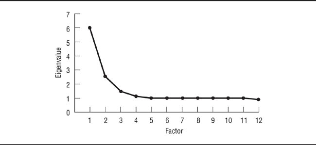
Plot of Eigenvalues for Exploratory Factor Analysis of Items in Box 12.1.

There are four eigenvalues greater than 1 and the plot levels off after Factor 4, indicating that four factors should be rotated.

A third approach, generally considered to be superior to the first two, is parallel analysis (Hayton, Allen, & Scarpello, 2004). In parallel analysis, researchers create a random data set with the same number of observations and variables as the real data set. They then conduct a factor analysis of the random data to compute the eigenvalues; because the random data set has the same number of variables as the real data, it will produce the same number of eigenvalues. This process is conducted at least 50 times to create a set of random eigenvalues. The researchers then compute the mean of each of the random eigenvalues and compare each mean random eigenvalue to its equivalent real eigenvalue. That is, the researchers compare mean random eigenvalue 1 with real eigenvalue 1, mean random eigenvalue 2 with real eigenvalue 2, and so forth. Only factors whose real eigenvalues are larger than the equivalent mean random eigenvalue are interpreted. The reasoning behind this procedure is that any real eigenvalues that are less than or equal to their mean random equivalues could have occurred by chance. In the sample factor analysis, all four eigenvalues that were greater than 1 were also larger than their mean random equivalents. Therefore, the eigenvalues-greater-than-1 rule, the scree plot, and parallel analysis all indicated that there were four factors in the sample data of Box 12.1.

Interpreting the factors. The result of an exploratory factor analysis is a matrix of factor loadings such as that shown in Table 12.1 for the sample analysis. The loadings represent the correlation of each item with the underlying factor; therefore, higher factor loadings show stronger associations with a factor. Most authorities hold that an item should have a loading of at least .30 to be considered part of a factor, although the stricter criterion of .40 is often used. As a practical matter, the cutoff for factor loadings can be set relative to the size of the loadings: A large number of high loadings justifies a higher cutoff. For example, 88% of the factor loadings greater than .30 in Table 12.1 are also greater than .50, so it would be reasonable to use .50 as a cutoff for this analysis. Therefore, we can say that Factor 1 consists of Items 1, 2, 3, 4, 5, 8, and 13; that Factor 2 consists of Items 6, 7, 9, 14, and 16; that Factor 3 consists of Items 10, 11, 12, 15, and 17; and that Factor 4 consists of Items 1, 18, 19, and 20.

TABLE 12.1

Results of an Exploratory Factor Analysis of the Items in Box 12.1

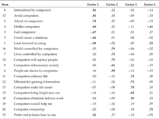
Having decided which variables load on which factors, you must decide what the factors mean—that is, what construct underlies the variables—and name the factors. Factor interpretation and naming are completely judgmental processes: You examine the items that load on a factor and try to determine the concept common to them, giving more weight to items that have higher absolute value factor loadings (that is, ignoring the factor loadings’ plus or minus signs). For example, Factor 1 in Table 12.1 appears to represent anxiety about using computers, Factor 2 appears to represent perceptions of computers’ negative impact on society, Factor 3 appears to represent perceptions of computers’ positive impact on society, and Factor 4 appears to represent the perceived personal utility of computers.

Note two characteristics of the factor loadings shown in Table 12.1. First, a loading can be either positive or negative; positive loadings indicate positive correlations with the factor, negative loadings indicate negative correlations. Typically, items with negative loadings are worded in the opposite direction of items with positive loadings. Consider, for example, Item 8, which loaded positively on Factor 1, and Item 3, which loaded negatively. A high score on Item 8 (“I feel intimidated by computers”) indicates a high degree of anxiety, whereas a high score on Item 3 (“I feel more competent working with computers than do most people”) indicates a low degree of anxiety.

The second notable characteristic of the factor loadings in Table 12.1 is that an item can load on more than one factor: Items 1, 4, 13, and 19 have loadings greater than .30 on both Factor 1 and Factor 4. A large number of items loading on two factors indicates that the factors are correlated and suggests that an oblique rotation might be appropriate for the data.

Factor scores. At the outset of this discussion of exploratory factor analysis, we noted that one of its purposes is to reduce a large number of variables to a smaller number. This is done by computing factor scores, respondents’ combined scores for each factor. Factor scores can be computed in two ways. The first is to have the factor analysis computer program generate factor score coefficients for the items. These coefficients are standardized regression coefficients that predict the factor score from Z scores on the items: Multiply each participant’s Z score on each item by its factor score coefficient for a factor, and sum the resulting products to obtain the participant’s factor score for that factor. Typically, one uses only the items that one considers to have loaded on the factor—that is, items with factor loadings above the cutoff. When all the items use the same rating scale (such as a 1-to-7 scale), you can use a simpler process: Reverse score items with negative loadings and sum participants’ scores on the items that load on each factor, just as one sums the scores on the items of a multi-item scale. You can then use factor scores as the dependent variables in other analyses of the data.

Exploratory factor analysis can be a very powerful tool for data reduction and for understanding the patterns of relationships among variables. However, it is also a very complex tool, and so you should undertake a factor analysis only after becoming familiar with the complexities of the technique and under the guidance of someone well-versed in its use.

Confirmatory Factor Analysis

Confirmatory factor analysis is, in a way, the mirror image of exploratory factor analysis. In exploratory factor analysis, one examines a set of item scores to see what dimensions underlie the items and which items load on which dimensions. In confirmatory factor analysis, one hypothesizes the dimensions a set of items will load on and uses statistical analyses to confirm (or refute) that hypothesis. Because confirmatory factor analysis is a form of factor analysis, many of the same statistical considerations apply to it, including adequate sample size, data quality, and lack of multicolinearity. Researchers use confirmatory factor analysis for two principal purposes, hypothesis testing and measure validation. Goodness-of-fit indices are used to assess how well these purposes are accomplished.

Hypothesis Testing

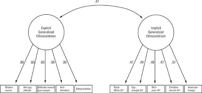
Different theories concerning a particular psychological phenomenon sometimes postulate different patterns of relationship among variables encompassed by the theories. For example, Cunningham, Nezlek, and Banaji (2004) were interested in whether different forms of prejudice—such as racial prejudice, anti-gay prejudice, and anti-Semitism—are expressions of a single psychological process (which they refer to as generalized ethnocentrism) or whether the different forms of prejudice are essentially unrelated because they spring from different psychological roots. Cunningham and colleagues also wanted to see if using explicit and implicit measures (see Chapter 6) of prejudice would produce the same results and how closely explicit and implicit generalized ethnocentrism were related to one another. They hypothesized that different forms of prejudice did, in fact, stem from generalized ethnocentrism and that explicit and implicit generalized ethnocentrism would be positively correlated. In factor analysis terms, they hypothesized that measures of different types of prejudice would load on two generalized ethnocentrism factors, one for the explicit measures and one for the implicit measures, and that the two factors would be correlated.

Cunningham and colleagues (2004) tested their hypotheses by collecting data from 206 research participants. Although this sample size is near the low end of recommendations made by experts (which range from 150 to 500; Schumacker & Lomax, 2004), it was nonetheless adequate. Participants completed self-report measures of prejudice against African Americans, prejudice against homosexuals, anti-Semitism, and ethnocentrism (prejudice against ethnic and nationality groups other than one’s own); their implicit attitudes toward these groups were assessed using the Implicit Association Test (see Chapter 6). Cunningham and colleagues also included some other variables in their study, but we will focus on their confirmatory factor analysis of prejudice measures.

Table 12.2 shows Cunningham and colleagues’ (2004) results in tabular form. Similar to the results of an exploratory factor analysis (see Table 12.1), the results of a confirmatory factor analysis can be presented as columns of factor loadings. However, because researchers using confirmatory factor analysis often (but not always) hypothesize that a variable will load on only one factor, no loadings are calculated for the other factors. As Table 12.2 shows, Cunningham and colleagues found the two factors they hypothesized, one for explicit measures and one for implicit measures, and that the two factors were positively correlated. Although confirmatory factor analysis allows one to test the statistical significance of factor loadings and inter-factor correlations, Cunningham and colleagues did not report that information. The researchers’ hypothesized model of the relationships among the variables they studied fit the data very well (we will discuss the concept of goodness-of-fit shortly), providing further support for their hypotheses. Their results indicate then, that various prejudices stem from a single psychological factor (generalized ethnocentrism), that this holds for both explicit and implicit prejudices, and that explicit and implicit generalized ethnocentrism are positively related.

TABLE 12.2

Results of Cunningham, Nezlek, and Banaji’s (2004) Confirmatory Factor Analysis of Types of Prejudice

	Explicit Generalized Ethnocentrism	Implicit Generalized Ethnocentrism
Modern racism	.68
Anti-gay attitudes	.63
Attitudes toward the poor	.63
Anti-Semitism	.68
Ethnocentrism	.90
Black-White IAT		.47
Gay-straight IAT		.49
Rich-poor IAT		.48
Christian-Jewish IAT		.47
American-foreign IAT		.57
Factor correlation	.47

Note:

IAT = Implicit Association Test (see Chapter 6). Data are from Cunningham et al. (2004), Figure 2.

Figure 12.3 presents Cunningham and colleagues’ (2004) results in the form of a diagram, in which rectangles represent observed variables (or measured variables), in this case the various prejudice measures, and the circles represent the latent variables (or factors) underlying the measured variables. The term latent variable refers to a variable that is not directly measured but which is estimated statistically from scores on measured variables. In a diagrammatic presentation of confirmatory factor analysis results, factor loadings are shown next to the arrows running from the latent variable to each of the measured variables; the direction of the arrows indicates that the latent variable is the hypothesized cause of the measured variables. The double-headed arrow between the latent variables indicates that those variables are hypothesized to be correlated and the correlation coefficient for that relationship is shown next to the arrow.

Measure Validation

In Chapter 6 we discussed several aspects of validity of measurement, including structural validity and generalizability. Confirmatory factor analysis can be used to assess both aspects.

FIGURE 12.3

Diagram of the Results of Cunningham, Nezlek, and Banaji’s (2004) Confirmatory Factor Analysis of Types of Prejudice.

Note: Error terms have been omitted for clarity. Rectangles represent the measured variables (the various measures) and the circles represent the latent variables (or factors) underlying the measured variables.

Structural validity. As you will recall, the concept of structural validity deals with the extent to which the dimensionality of a measure reflects the dimensionality of the construct it is measuring. The initial assessment of the structural validity of a new measure is based on an exploratory factor analysis of scores on a preliminary set of items. This analysis reveals the basic structure that underlies a set of items; to the extent that this structure matches the structure proposed by the theory of the construct being measured, there is evidence for structural validity. Confirmatory factor analysis provides additional evidence of structural validity by using data from new samples of research participants to determine if the factor structure revealed by the exploratory factor analysis can be replicated. The hypothesis in the replication research is that factor structure found in the exploratory factor analysis will be replicated in the new data set. The results of such a confirmatory factor analysis can be presented in either tabular or diagrammatic form as in Table 12.1 and Figure 12.3, with the items on the measure being treated as the measured variables. As with the case of hypothesis testing, goodness-of-fit indices allow one to assess how well the factor structure in the new data set matches the hypothesized structure and the statistical significance of the loadings can be tested.

Generalizability. Generalizability of measurement refers to the extent to which a measure provides similar results across time, research settings, and populations. As we saw in Chapters 6 and 8, differential validity—a situation in which a measure exhibits greater validity for one population group than another—is an important concern in the generalizability of measurement, especially in the cross-cultural context. To be cross-culturally valid, a measure should (among other characteristics) have an equivalent structure in the populations in which it is used (Chen, 2008). Confirmatory factor analysis can be used to assess cross-cultural generalizability by testing the invariance (or similarity) of a measure’s structure across groups (e.g., Byrne, 2010). To test structural invariance, one starts with a hypothesized structure, usually the structure found for the population in which the measure was first developed, say U. S. college students. One then collects a new set of data from that population and from the new population in which the measure is to be used, say English-speaking Chinese college students in Hong Kong. A confirmatory factor analysis is conducted for the data in both groups and the equality of various structural parameters from the confirmatory factor analyses, such as factor loadings and inter-factor correlations, is tested statistically. Equality of parameters across groups indicates that the structure of the measure generalizes across those groups.

Evaluating Goodness of Fit

One means of evaluating the success of a confirmatory factor analysis is by assessing a confirmatory factor analysis model’s goodness-of-fit. The concept of goodness-of-fit derives from the fact that confirmatory factor analysis tests a hypothesized factor structure against the structure that exists in a data set. The fit (or match) between the hypothesized structure and the actual structure is one indicator of the accuracy of the hypotheses. There are a large number of statistical indexes that one can use to assess model fit, each of which has its strengths and limitations (e.g., Byrne, 2010; Schumacker & Lomax, 2004). However, four seem to be the most commonly used (Thompson, 2004): the chi-square test, the root mean square error of approximation (RMSEA), the normed fit index (NFI), and the comparative fit index (CFI). Because only the chi-square test can be evaluated for statistical significance, researchers commonly calculate several goodness-of-fit indices and evaluate a model based on the extent to which they agree.

The chi-square test and RMSEA evaluate the degree to which the parameters of a model can reproduce aspects of the data: the better the degree of reproduction, the more accurate the model. Because the ideal fit is no difference between the reproduced and actual data, in the best case χ² would equal zero; in practice, a statistically non-significant X² value is considered indicative of a good fitting model. One shortcoming of the chi-square test is that it is sensitive to sample size, such that, all else being equal, larger samples produces larger χ² values. As a result, in some cases models that, in fact, fit the data well produce statistically significant χ² values. In contrast, RMSEA is not sensitive to sample size but cannot be tested for statistical significance. There are, however, guidelines for evaluating RMSEA. Like χ², RMSEA should ideally be zero, with values less than or equal to .05 indicating a good fit, values greater than .05 but less than or equal .10 indicating an adequate fit, and values greater than .10 indicating a poor fit.

The NFI and CFI take a different approach to assessing fit. The null hypothesis for a confirmatory factor analysis model is that none of the variables are related to any of the others. The NFI and CFI compare the model found in the CFA to this null model. In contrast to the chi-square test and RMSEA of approximation, for NFI and CFI larger values are better, to a maximum possible value of 1.0. As with RMSEA, NFI and CFI cannot be tested for statistical significance, but evaluation guidelines exist: values greater than or equal to .95 indicate a good fit, values greater than .90 but less than .95 indicate an adequate fit, and values less than .90 indicate a poor fit.

Cunningham and colleagues (2004) used the chi-square test, RMSEA, NFI, and CFI to evaluate the results of their confirmatory factor analysis. They found that χ²(29) =17.29 (which was not statistically significant), RMSEA = 0.00, NFI = 1.00, and CFI = 1.00. Taken together, the results of these tests indicated a model with an excellent fit to the data, and so the researchers could have great confidence that in their results. Finally, one can compare how well two confirmatory factor analysis models fit the same data. Recall that Cunningham and colleagues (2004) hypothesized that there would be a correlation between the explicit and implicit generalized ethnocentrism factors. In confirmatory factor analysis, one can test such a hypothesis by comparing the fit of a model without correlated factors to a model that includes correlated factors by comparing the chi-square values for the models; because a difference in chi-squares is also a chi-square value, a model that has a significantly smaller χ² value fits the data better than a competing model. Cunningham et al. used this technique and found that the difference χ²(1) = 71.44, p .001, confirming their hypothesis of correlated factors.

Testing Mediational Hypotheses

In addition to testing the factor structure of a set of variables, correlational methods can be used to test mediational hypotheses; in fact, as we will see, confirmatory factor analysis is part of one such method. As we noted in Chapter 1, theories do not always postulate direct relationships between variables. Instead, they sometimes postulate that an independent variable (I) affects a mediating variable (M), which in turn affects the dependent variable (D); that is, I → M → D. For example, Condon and Crano (1988) postulated that the well-established relationship between attitude similarity and liking—the more similar someone’s attitudes are to our own, the more we like the person—is mediated by a third variable, the assumption that the other person likes us. That is, similarity → assumed reciprocity of liking → attraction. In this section, we discuss some ways in which such mediational models can be tested: the causal steps strategy, path analysis, and structural equation modeling.

The Causal Steps Strategy

Condon and Crano’s (1988) model is an example of the simplest form of mediation, one involving only three variables. A mediational situation potentially exists when I is correlated with both D and M and when M is correlated with D (Baron & Kenny, 1986; Judd & Kenny, 2010; Kenny, Kashy, & Bolger, 1998). Simple mediation is often tested using the causal steps strategy for testing, which employs a set of multiple regression analyses. The steps of this analysis are:

•	Compute the unstandardized regression coefficient for the relationship between I and M (this is coefficient a).
•	Compute the unstandardized regression coefficient for the relationship between M and D (this is coefficient b).
•	Multiply coefficient a by coefficient b (= ab) and divide this product by its standard error (see Kenny et al., 1998, p. 260, for the formula for the standard error); this procedure is called the Sobol test. If ab is statistically significant, one can conclude that M mediates the relationship between I and D.

As an example of the use of this method, consider Preacher and Hayes’s (2008) analysis of data from Kalyanaraman and Sundar’s (2006) study of factors that influence Internet users’ preferences for Web portals. One of Kalyanaraman and Sundar’s hypotheses was that liking for a Web portal was a function of the extent to which users perceived the portal to be customized to their needs. They also hypothesized that users’ perceptions of the control they had over interactions with the portal would mediate the relationship between perceived customization and liking; that is, higher perceived customization —> higher perceived control —> greater liking for the portal. Using Kalyanaraman and Sundar’s data, Preacher and Hayes calculated the unstandardized regression coefficient for the relationship between perceived customization and perceived control (coefficient a) to be 0.401 and the unstandardized regression coefficient for the relationship between perceived control and liking for a portal to be 0.301 (coefficient b), with ab = 0.121. The standard error for ab was 0.044, so that ab divided by its standard error was 2.733, p = .006; these results support the mediational hypothesis.

Path Analysis

Mediational models only sometimes take the form of the simple three-variable case; more commonly, mediational models hypothesize more than one mediating variable. Such models may propose that two or more variables mediate the relationship between an independent and dependent variables, as is the case with the model shown in Figure 12.4 (which we will discuss shortly). Mediational hypotheses may also propose causal chains, such as I → M₁ → M₂ → D, or a combination of simultaneous and sequential mediators. Models such as these can be tested using path analysis. Path analysis can also be used in prospective research to examine patterns of correlation across time. Finally, path analysis can be combined with confirmatory factor analysis to permit path analysis of relationships using latent variables.

Path analysis uses sets of multiple regression analyses to estimate the strength of the relationship between an independent variable and a dependent variable controlling for the hypothesized mediating variables. This method is called path analysis because the lines indicating the hypothesized relationships in diagrams such as Figure 12.4 are referred to as paths, and the regression coefficients for the relationships as path coefficients. The terms causal analysis or causal modeling are also sometimes used to refer to path analysis; however, these terms are misleading because, although the models do represent hypothesized causal relationships, they are most often tested using correlational methods. One can only draw causal conclusions from them when one or more of the independent variables included in the analysis has been manipulated. In those cases, only the results for the manipulated variable can be interpreted in causal terms.

FIGURE 12.4

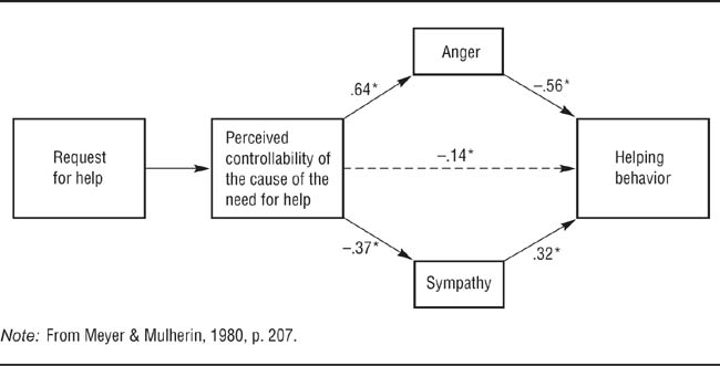
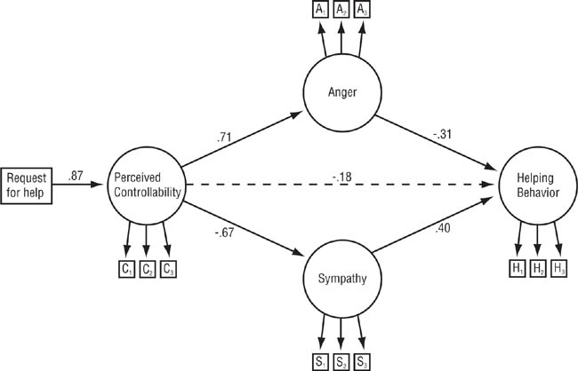
Path Analysis Diagram for Meyer and Mulherin’s (1980) Analysis of the Attributional Model of Response to a Request for Help.

Causes perceived to be controllable lead to more anger and less sympathy, which lessen the likelihood of helping.

Consider the model shown in Figure 12.4, in which arrows lead from hypothesized causes to their effects. Drawing on Weiner’s (1986) attribution theory, Meyer and Mulherin (1980) postulated that the way in which Person A responds to a request for help from Person B depends on the degree to which Person A perceives the cause of Person B’s need for help to be under Person B’s control: the greater the perceived controllability, the less likely Person A is to help. However, the theory also holds that the relationship between perceived controllability and helping is mediated by Person A’s emotional responses of anger and sympathy. Models such as these are tested statistically in two ways. First, the significance of each hypothesized path (indicated by solid lines in Figure 12.4) is tested, and any possible paths that are hypothesized not to exist, such as the path from controllability directly to helping in Meyer and Mulherin’s (1980) model (indicated by the broken line in Figure 12.4), should also be tested to ensure that they are not significant. Second, equations can be developed to reconstruct the correlation matrix for the variables from the path coefficients and the reconstruction can be evaluated using the same goodness-of-fit indexes used in confirmatory factor analysis. There are a number of statistical computer packages that can be used to analyze data for path models (e.g., Byrne, 2010; Schumacker & Lomax, 2004).

In Meyer and Mulherin’s (1980) research, participants read one of several scenarios and were instructed to imagine that an acquaintance asked for a loan to help pay for his or her rent. In these scenarios, perceptions of controllability were manipulated by changing the supposed cause of the need for a loan. For example, in one scenario the acquaintance said that he was short of money because he had missed work due to illness (an uncontrollable cause). In another scenario, he said that he had missed work because he had not felt like go to a work for a few days (a controllable cause). The participants then rated the scenarios they read on how controllable they thought the cause of the acquaintance’s need was, how angry and sympathetic they felt toward the acquaintance, and how likely they would be to lend the acquaintance money. The researchers found a zero-order correlation of r =-.62 between perceptions of controllability and likelihood of helping, indicating that participants who saw the cause of the need as more controllable said that they would be less likely to help. However, as shown in Figure 12.4, Meyer and Mulherin also found that feelings of anger and sympathy mediated the relationship between perceived controllability and likelihood of helping: With anger and sympathy controlled, the relationship between anger and controllability was reduced to r = -.14.

Structural Equation Modeling

Structural equation modeling (SEM) combines path analysis with confirmatory factor analysis (Kaplan, 2000). SEM applies confirmatory factor analysis to multiple measures of each construct used in a path model to estimate for each research participant a latent variable score representing the construct. For example, each participant might complete three depression inventories (manifest variables), which jointly represent the latent variable of depression. Latent variables are assumed to be measured with less error than are any of the individual observed variables; the rationale is that true score variance on the latent variable that is missed by one manifest variable will be picked up by another. The technique then estimates the path coefficients for the relationships among the latent variables.

FIGURE 12.5

Results of Reisenzein’s (1986) Latent Variables Path Analysis of the Attributional Model of Response to a Request for Help.

Compare with the results of Meyer and Mulherin’s (1980) observed-variables path analysis shown in Figure 12.4.

For example, Reisenzain (1986) used SEM to replicate Meyer and Mulherin’s (1980) path analysis of Weiner’s model of helping behavior. His results are shown in Figure 12.5. Like Meyer and Mulherin, Reisenzein used an experimental manipulation to create different levels of perceived controllability of the need for help. He measured each variable in the model—perceived controllability, sympathy for the person needing help, anger toward the person needing help, and likelihood of helping the person—with three items. These items are indicated in Figure 12.5 by the squares labeled C1, C2, and so forth; arrows lead from the ovals representing the latent variables to the squares representing the items for those variables because the unobserved latent variables are assumed to cause the observed item scores.

Reisenzein (1986) evaluated the fit of his model using the chi-square test and the Bentler-Bonett Index (BBI), which is interpreted in the same way as the normed fit index described earlier. Reisenzein found that χ²(58) = 67.28 (which was not statistically significant) and that BBI = 0.95. The values of both of these indexes indicate that the model fit the data well. If you compare Figure 12.6 with Figure 12.4, you can see that Reisenzein’s research replicated Meyer and Mulherin’s (1980) results. Although the path coefficients are not identical (and one would not expect them to be given the methodological differences between the studies), the pattern of results is the same: Perceptions of controllability lead to more anger (indicated by the positive path coefficient) and less sympathy (indicated by the negative path coefficient) and increased anger led to decreased intentions to help whereas increased sympathy led to increased intentions to help.

FIGURE 12.6

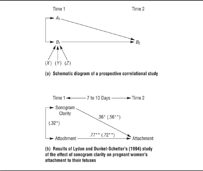
Prospective Correlation Analysis.

A significant path coefficient from A1 to B2 indicates that Variable A may have time precedence over Variable Bs

Prospective Research

Prospective research examines the correlation of a hypothesized cause at Time 1 with its hypothesized effect at Time 2 to investigate the time precedence of a possible causal variable (Barnett & Gotlib, 1988). As shown in panel (a) of Figure 12.6, this kind of analysis takes the form of a path model. Variable B at Time 2 (B₂) has at least two possible causes, Variable A at Time 1 (A₁) and Variable B at Time 1 (B₁); the double-headed arrow represents their correlation. B₁ is included as a cause of B₂ for two reasons. First, B₁ is an extraneous variable relative to A₁ and an alternative explanation to A₁ as a cause of scores on B₂ because people who score high on Variable B at Time 1 are likely to score high on Variable B at Time 2, regardless of the effects of Variable A. Second, B₁ represents other, unmeasured, causes of Variable B—Variables X, Y, and Z in Figure 12.6. It would be best, of course, to include Variables X, Y, and Z directly in the model as extraneous variables, but they might be either unknown or too difficult to measure. The question, then, is whether if, with B₁ controlled, A₁ has a significant relationship to B₂; in other terms, is the partial correlation of A₁ with B₂controlling for B₁ greater than zero?

For example, panel (b) of Figure 12.6 shows the results of a study conducted by Lydon and Dunkel-Schetter (1994). These researchers wanted to know if the clarity of a sonogram increased pregnant women’s feelings of attachment to their fetuses. They measured the women’s feelings of attachment immediately prior to the mothers’ undergoing an ultrasound examination and immediately afterward measured the clarity of the sonogram (which the mothers saw in real time) by asking the mothers to list the parts of the fetus’s body that they had seen. Clarity was operationally defined as the number of body parts listed. Attachment was again measured 7 to 10 days after the examination. As shown in panel (b) of Figure 12.6, Time 1 level of attachment was correlated with sonogram clarity (r = .32), indicating that women with higher initial attachment levels reported having seen more body parts; attachment at Time 1 was also highly correlated with attachment at Time 2 (r = .77). Sonogram clarity had a zero-order correlation of r = .56 with attachment at Time 2, and the significant path coefficient of .36 indicated that clarity could explain 12% of the variance in Time 2 attachment in addition to the variance explainable by presonogram attachment. Thus, mothers who reported seeing more fetal body parts during their ultrasound examinations had higher levels of attachment to their fetuses at Time 2 than did mothers who reported seeing fewer body parts even when initial level of attachment was controlled. By the way, initial level of attachment was high for all mothers, averaging 3.7 on a 5-point scale.

Although prospective correlational research can be useful in identifying the potential time precedence of one variable over another, one must draw conclusions cautiously: Some unmeasured third variable may be the cause of Variable A and thus be the ultimate, hidden, cause of variable B (Cook & Campbell, 1979). In addition, as discussed next, path analysis and SEM have a number of limitations that one must always take into account.

Limitations on Interpretation

Although path analysis and SEM can be an extremely useful data analysis tools, there are a number of limitations on the interpretation of their results (Cliff, 1983). We want to emphasize two of them.

Completeness of the model. The first limitation deals with the completeness of the model being tested. The issue of completeness includes two questions: (a) Are all relevant variables included? (b) Are there any curvilinear or nonadditive relationships? Because path analysis and SEM examine the patterns of partial correlations among variables, addition or deletion of a variable, or omission of an important variable, can radically change the pattern of results. Scarr (1985) provides an example of this situation. She first shows that a model predicting children’s IQ scores at age 48 months from maternal positive discipline and positive control (for example, use of reasoning rather than physical punishment) adequately fits data collected from 125 families—panel (a) in Figure 12.7. However, if maternal IQ scores and educational level are added to the model as hypothesized causes of discipline and control, then the only significant predictor of child IQ score is maternal IQ score—panel (b) in Figure 12.7. Maternal IQ score is correlated with both discipline and control, and it is more highly correlated with child IQ score than are the other two variables. Therefore, with maternal IQ score partialed out, discipline and control have no relationships to child IQ score. You should therefore be certain that all relevant variables are included in a path or SEM model before conducting the analysis. Note that including variables that are not relevant (but might be) will not change the conclusions drawn from the analysis. For example, Scarr (1985) goes on to show that the ability of maternal positive discipline to predict child’s social adjustment is not substantially reduced by adding maternal IQ score and educational level to the model.

FIGURE 12.7

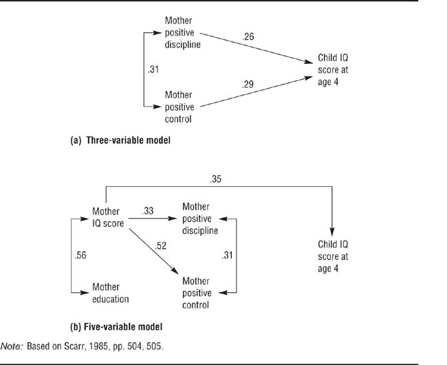
Effect of Adding Variables in a Path Model.

Adding mother IQ score and mother education to the model makes the paths from mother positive discipline and mother positive control to child IQ score at age 4 nonsignificant. Nonsignificant paths have been omitted for clarity.

Most path and SEM models assume strict linearity and additivity; that is, they do not consider the possibility of curvilinear relationships or interactions. It is possible to include such factors in path models, but they can be difficult to compute and interpret (e.g., Schumacker & Lomax, 2004). If different models are hypothesized for different participant groups or experimental conditions, separate path models can be tested for each group or condition (e.g., Elliot & Harackiewicz, 1994). One can then test whether the two models are different, which would support the interaction hypothesis, or similar, which would contradict the hypothesis (e.g., Byrne, 2010).

Alternative models. The second limitation on the interpretation of path analyses and SEM concerns the fit of a model to the data: It is entirely possible that more than one model will fit the data equally well (Breckler, 1990). For example, considerable research has been conducted on the relationship between religious fundamentalism and prejudice. Generally, people who score high on fundamentalism also score high on prejudice, although the size of the correlation has been diminishing over time (Hall, Matz, & Wood, 2010). One explanation that has been proposed for the relationship is that fundamentalism is related to prejudice because it is also related to right-wing authoritarianism, a social ideology that is also related to prejudice (e.g., Whitley & Kite, 2010). However, as shown in Figure 12.8, there are at least three ways in which fundamentalism, authoritarianism, and prejudice could be related to one another: (a) being raised in a fundamentalist religion increases the likelihood of a person’s acquiring an authoritarian ideology, which then leads to prejudice; (b) authoritarianism and fundamentalism are correlated with each other although neither causes the other and either both are possible causes of prejudice or only one remains as a possible cause after the other is controlled; and (c) authoritarianism, fundamentalism, and prejudiced are intercorrelated because all are caused by an unknown third variable. The implication of this example is that when conducting a path analysis or SEM you should test not only your preferred model but also any plausible alternative models. These alternatives include different arrangements of possible causal sequences, including reverse causation and reciprocal causation.

FIGURE 12.8

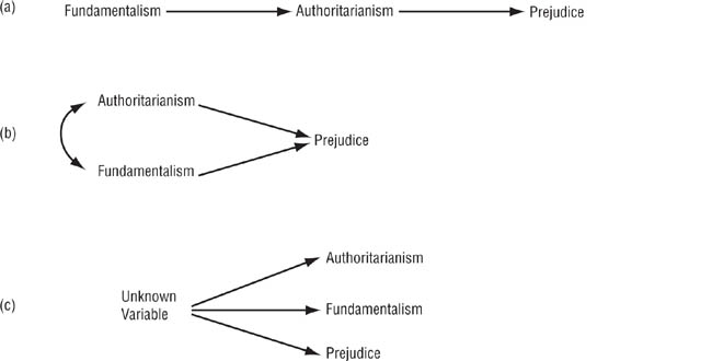
Three Theoretical Models of the Relationships Among Religious Fundamentalism, Right-Wing Authoritarianism, and Prejudice.

Bear in mind that some alternative models might be ruled out by logic (for example, weight cannot cause height) or prospective correlations (for example, if Variable A does not predict Variable B across time, Variable A does not have time precedence over Variable B). In addition, sometimes experiments can be designed to eliminate specific causal possibilities or to demonstrate causality. In fact, it is not uncommon for the independent variable in a path model to be a manipulated variable. For example, Condon and Crano (1988) manipulated the apparent similarity in attitudes between the participants in their research and the person the participants were evaluating, and Meyer and Mulherin (1980) and Reisenzein (1986) manipulated the reason why the person described in the scenario needed help. Under these conditions, one can conclude that the independent variable causes the mediating and dependent variables. What one cannot conclude with certainty is that the mediating variable causes the dependent variable, only that the mediating variable is correlated with the dependent variable. However, other research that manipulates the mediating variable as an independent variable could reveal a causal relationship.

Chapter Summary

Factor analysis consists of a set of statistical techniques used to examine the relationships among a set of intercorrelated variables. Exploratory factor analysis examines the pattern of correlations to find subsets of variables whose members are related to one another and are independent of the other subsets. It is used to reduce a larger number of variables to a smaller number for data analysis and to determine if the items on a scale represent one or more than one construct. Important considerations in factor analysis include having an adequate sample size, having a set of variables that are strongly intercorrelated but not multicollinear, choice of factor extraction and rotation methods, determining the number of factors to interpret, and the interpretation of those factors. In confirmatory factor analysis, one hypothesizes the dimensions responses to a set of items will load on and uses statistical analyses to confirm (or refute) that hypothesis. Confirmatory factor analysis can test hypotheses about the relations among sets of variables and can be used to evaluate the structural validity and generalizability of a measure. One can evaluate the success of a confirmatory factor analysis using a variety of goodness-of-fit indexes.

Mediational models hypothesize that an independent variable causes a mediating variable which, in turn, is the cause of the dependent variable. Simple, three variable hypotheses can be tested using the causal steps strategy, which is based on multiple regression analysis. More complex hypotheses are tested using path analysis or structural equation modeling, which combines path analysis with confirmatory factor analysis to examine relationships among unmeasured latent variables derived from confirmatory factor analyses of multiple measures of the variables. Path and structural equation models can also be used to test the time precedence of a proposed causal variable. When interpreting the results of path analyses, it is essential to ensure that the model being tested is complete and that no alternative models fit the data.

Suggestions for Further Reading

Factor Analysis

Bryant, F. B., & Yarnold, P. R. (1995). Principal-components analysis and exploratory and confirmatory factor analysis. In L. G. Grimm & P. R. Yarnold (Eds.),Reading and understanding multivariate statistics (pp. 99-136). Washington, DC: American Psychological Association.

Fabrigar, L. R., Wegener, D. T., MacCallum, R. C., & Strahan, E. J. (1999). Evaluating the use of exploratory factor analysis in psychological research.Psychological Methods, 4(3), 272–299.

Thompson, B. (2004).Exploratory and confirmatory factory analysis: Understanding concepts and applications. Washington, DC: American Psychological Association.

Bryant and Yarnold and Thompson provide very readable introductions to exploratory and confirmatory factor analysis (CFA). Byrne (2010) and Schumacker and Lomax (2004), below, provide more detailed discussion of CFA with examples. Fabrigar and colleagues discuss the choices researchers must make when conducting an exploratory factor analysis.

Testing Mediational Models

MacKinnon, D. P. (2008).Introduction to statistical mediation analysis. New York: Psychology Press.

Preacher, K. J., & Hayes, A. F. 2008). Contemporary approaches to assessing mediation in communication research. In A. F. Hayes, M. D. Slater, & L. B. Snyder (Eds.),Sage sourcebook of advanced data analysis methods for communication research (pp. 13–54). Los Angeles, CA: Sage.

MacKinnon provides a detailed introduction to conducting mediational analyses. Preacher and Hayes review the advantages and limitations of various methods for testing mediational models.

Path Analysis and Structural Equation Modeling

Byrne, B. M. (2010). Structural equation modeling with AMOS: Basic concepts, applications, and programming (2nd ed.) New York: Routledge.

Klem, L. (1995). Path analysis. In L. G. Grimm & P. R. Yarold (Eds.), Reading and understanding multivariate statistics (pp. 65–97). Washington, DC: American Psychological Association.

Klem, L. (2000). Structural equation modeling. In L. G. Grimm & P. R. Yarold (Eds.), Reading and understanding more multivariate statistics (pp. 227–260). Washington, DC: American Psychological Association.

Schumacker, R. E., & Lomax, R. G. (2004).A beginner’s guide to structural equation modeling (2nd ed.). New York: Psychology Press.

Klem provides very readable introductions to path analysis with observed variables (1995) and its counterpart using latent variables, structural equation modeling (SEM; 2000). Byrne and Schumacker and Lomax provide more detailed information along with examples using the most popular SEM computer programs.

Key Terms

Causal steps strategy

Confirmatory factor analysis

Eigenvalue

Exploratory factor analysis

Factor (in factor analysis)

Factor analysis

Factor loading

Factor score

Goodness-of-fit

Latent variable

Observed variable

Parallel Analysis

Path analysis

Prospective research

Scree plot

Structural equation modeling

Questions for Review and Discussion

1.	What is factor analysis? What is the difference between exploratory and confirmatory factor analysis?
2.	How is exploratory factor analysis used in research? What are the important issues to consider when conducting an exploratory factor analysis?
3.	Find an exploratory factor analysis that was conducted in a research area that interests you. How well did the researchers meet the conditions for a good factor analysis? Explain in your own words the goal of the factor analysis and the meaning of the results the researchers obtained.
4.	How is confirmatory factor analysis used in research?
5.	Find a confirmatory factor analysis that was conducted in a research area that interests you. How well did the researchers meet the conditions for a good factor analysis? Explain in your own words the goal of the factor analysis and the meaning of the results the researchers obtained.
6.	What does the term goodness-of-fit mean? What is its role in confirmatory factor analysis and path analysis?
7.	What is a mediational hypothesis? How does a mediational hypothesis differ from one that proposes a moderating variable? How can mediational hypotheses be tested in research?
8.	What is path analysis? Find a path analysis that was conducted in a research area that interests you. Explain in your own words the goal of the path analysis and the meaning of the results the researchers obtained.
9.	What is prospective research? What role does path analysis play in prospective research?
10.	What is a latent variable? How does structural equation modeling differ from path analysis?
11.	What issues should one bear in mind when interpreting the results of a path analysis?
12.	Think back to Chapter 9, in which we discussed how to test hypotheses about the effects of moderator variables. How does the concept of moderation differ from the concept of mediation? What is the most appropriate way in which to the effect of a hypothesized moderator variable?