
As you saw in Chapter 8, algebraic functions not only produce straight lines but curved ones too. A special type of curved function is called a parabola. Perhaps you have seen the shape of a parabola before:
Many real life situations model a quadratic equation. This chapter will explore the graph of a quadratic equation and how to solve such equations using various methods.

Chapter 9 introduced the concept of factoring quadratic trinomials of the form ![]() . This is also called the standard form for a quadratic equation. The most basic quadratic equation is
. This is also called the standard form for a quadratic equation. The most basic quadratic equation is ![]() . The word quadratic comes from the Latin word quadrare, meaning “to square.” By creating a table of values and graphing the ordered pairs, you find that a quadratic equation makes a
. The word quadratic comes from the Latin word quadrare, meaning “to square.” By creating a table of values and graphing the ordered pairs, you find that a quadratic equation makes a ![]() -shaped figure called a parabola.
-shaped figure called a parabola.
|
|
|
| –2 | 4 |
| –1 | 1 |
| 0 | 0 |
| 1 | 1 |
| 2 | 4 |

A parabola can be divided in half by a vertical line. Because of this, parabolas have symmetry. The vertical line dividing the parabola into two equal portions is called the line of symmetry. All parabolas have a vertex, the ordered pair that represents the bottom (or the top) of the curve.
The vertex of a parabola has an ordered pair ![]() .
.

Because the line of symmetry is a vertical line, its equation has the form ![]() , where
, where ![]() the
the ![]() coordinate of the vertex.
coordinate of the vertex.
An equation of the form ![]() forms a parabola.
forms a parabola.
If ![]() is positive, the parabola will open upward. The vertex will be a minimum.
is positive, the parabola will open upward. The vertex will be a minimum.
If ![]() is negative, the parabola will open downward. The vertex will be a maximum.
is negative, the parabola will open downward. The vertex will be a maximum.
The variable ![]() in the equation above is called the leading coefficient of the quadratic equation. Not only will it tell you if the parabola opens up or down, but it will also tell you the width.
in the equation above is called the leading coefficient of the quadratic equation. Not only will it tell you if the parabola opens up or down, but it will also tell you the width.
If ![]() or
or ![]() , the parabola will be narrow about the line of symmetry.
, the parabola will be narrow about the line of symmetry.
If ![]() , the parabola will be wide about the line of symmetry.
, the parabola will be wide about the line of symmetry.
Example 1: Determine the direction and shape of the parabola formed by ![]() .
.
Solution: The value of ![]() in the quadratic equation is –1.
in the quadratic equation is –1.
Several times throughout this textbook, you have experienced the terms domain and range. Remember:
The domain of every quadratic equation is all real numbers ![]() . The range of a parabola depends upon whether the parabola opens up or down.
. The range of a parabola depends upon whether the parabola opens up or down.
If ![]() is positive, the range will be
is positive, the range will be ![]() .
.
If ![]() is negative, the range will be
is negative, the range will be ![]() , where
, where ![]() coordinate of the vertex.
coordinate of the vertex.
Compare the five parabolas to the right. What do you notice?

The five different parabolas are congruent with different ![]() intercepts. Each parabola has an equation of the form
intercepts. Each parabola has an equation of the form ![]() , where
, where ![]() and
and ![]() intercept. In general, the value of
intercept. In general, the value of ![]() will tell you where the parabola will intersect the
will tell you where the parabola will intersect the ![]() axis.
axis.
The equation ![]() is a parabola with a
is a parabola with a ![]() intercept of
intercept of ![]() .
.
The vertical movement along a parabola’s line of symmetry is called a vertical shift.
Example 1: Determine the direction, shape, and ![]() intercept of the parabola formed by
intercept of the parabola formed by ![]() .
.
Solution: The value of ![]() in the quadratic equation is
in the quadratic equation is ![]() .
.
Projectiles are often described by quadratic equations. When an object is dropped from a tall building or cliff, it does not travel at a constant speed. The longer it travels, the faster it goes. Galileo described this relationship between distance fallen and time. It is known as his kinematical law. It states the “distance traveled varies directly with the square of time.” As an algebraic equation, this law is:
![]()
Use this information to graph the distance an object travels during the first six seconds.
|
|
|
| 0 | 0 |
| 1 | 16 |
| 2 | 64 |
| 3 | 144 |
| 4 | 256 |
| 5 | 400 |
| 6 | 576 |

The parabola opens upward and its vertex is located at the origin. The value of ![]() , so the graph is narrow about its line of symmetry. However, because the values of the dependent variable
, so the graph is narrow about its line of symmetry. However, because the values of the dependent variable ![]() are very large, the graph is misleading.
are very large, the graph is misleading.
Example 2: Anne is playing golf. On the fourth tee, she hits a slow shot down the level fairway. The ball follows a parabolic path described by the equation, ![]() , where
, where ![]() distance in feet from the tee and
distance in feet from the tee and ![]() height of the golf ball, in feet.
height of the golf ball, in feet.
Describe the shape of this parabola. What is its ![]() intercept?
intercept?
Solution: The value of ![]() in the quadratic equation is –0.04.
in the quadratic equation is –0.04.
The distance it takes a car to stop (in feet) given its speed (in miles per hour) is given by the function ![]() . This equation is in standard form
. This equation is in standard form ![]() , where
, where ![]() , and
, and ![]() .
.
Graph the function by making a table of speed values.

|
|
|
| 0 | 0 |
| 10 | 15 |
| 20 | 40 |
| 30 | 75 |
| 40 | 120 |
| 50 | 175 |
| 60 | 240 |
Using the function to find the stopping distance of a car travelling 65 miles per hour yields:
![]()
Multimedia Link: For more information regarding stopping distance, watch this CK-12 Basic Algebra: Algebra Applications: Quadratic Functions

Forensics. The distance a car travels even after the brakes are applied can be described through a quadratic function. But there is also the reaction time, the split second before the brakes are applied. The total distance is known as the stopping distance and this segment analyzes the quadratic function. (Click here to watch the video)
- YouTube video.
Sample explanations for some of the practice exercises below are available by viewing the following video. Note that there is not always a match between the number of the practice exercise in the video and the number of the practice exercise listed in the following exercise set. However, the practice exercise is the same in both. CK-12 Basic Algebra: Graphs of Quadratic Functions (16:05)
Graphs of Quadratic Functions (Click here to watch the video)
}

Graph the following equations by making a table. Let ![]() . Determine the range of each equation.
. Determine the range of each equation.
Which has a more positive ![]() intercept?
intercept?
Identify the vertex and ![]() intercept. Is the vertex a maximum or a minimum?
intercept. Is the vertex a maximum or a minimum?
Does the graph of the parabola open up or down?
Which equation has a larger vertex?
Graph the following functions by making a table of values. Use the vertex and ![]() intercepts to help you pick values for the table.
intercepts to help you pick values for the table.


Mixed Review
Isaac Newton’s theory for projectile motion is represented by the equation:
![]()
Consider the following situation: “A quarterback throws a football at an initial height of 5.5 feet with an initial velocity of 35 feet per second.”
By substituting the appropriate information:
The equation becomes ![]() .
.
Using the concepts from the previous lesson, we know
At what time will the football be 6 feet high? This equation can be solved by graphing the quadratic equation.
Chapter 7 focused on how to solve systems by graphing. You can think of this situation as a system:  . You are looking for the appropriate
 ![]() coordinates that give a
coordinates that give a ![]() coordinate of 6 feet. Therefore, you are looking for the intersection of the two equations.
coordinate of 6 feet. Therefore, you are looking for the intersection of the two equations.
Begin by typing the equations into the ![]() menu of your calculator. Adjust the window until you see the vertex,
menu of your calculator. Adjust the window until you see the vertex, ![]() intercept,
intercept, ![]() intercepts, and the horizontal line of 6 units.
intercepts, and the horizontal line of 6 units.


By looking at the graph, you can see there are two points of intersection. Using the methods from chapter 7, find both points of intersection.
![]()
At 0.014 seconds and again at 2.17 seconds, the football is six feet from the ground.
You can also use a graphing calculator to determine the vertex of the parabola. The vertex of this equation is a maximum point, so in the [CALCULATE] menu of the graphing option, look for [MAXIMUM].

Choose option #4. The calculator will ask you, “LEFT BOUND?” Move the cursor to the left of the vertex and hit [ENTER].
The calculator will ask, “RIGHT BOUND?” Move the cursor to the right of the vertex and hit [ENTER].
Hit [ENTER] to guess.
The maximum point on this parabola is (1.09, 24.64).
Example 1: Will the football reach 25 feet high?
Solution: The vertex represents the maximum point of this quadratic equation. Since its height is 24.64 feet, we can safely say the football will not reach 25 feet.
Example 2: When will the football hit the ground, assuming no one will catch it?
Solution: We know want to know at what time the height is zero.  . By repeating the process above and finding the intersection of the two lines, the solution is (2.33, 0). At 2.33 seconds, the ball will hit the ground.
The point at which the ball reaches the ground ![]() represents the
represents the ![]() intercept of the graph.
intercept of the graph.
The ![]() intercept of a quadratic equation is also called a root, solution, or zero.
intercept of a quadratic equation is also called a root, solution, or zero.
Example: Determine the number of solutions to ![]() .
.
Solution: Graph this quadratic equation, either by hand or with a graphing calculator. Adjust the calculator’s window to see both halves of the parabola, the vertex, the ![]() axis, and the
axis, and the ![]() intercept.
intercept.
The solutions to a quadratic equation are also known as its ![]() intercepts. This parabola does not cross the
intercepts. This parabola does not cross the ![]() axis. Therefore, this quadratic equation has no real solutions.
axis. Therefore, this quadratic equation has no real solutions.

Example: Andrew has 100 feet of fence to enclose a rectangular tomato patch. He wants to find the dimensions of the rectangle that encloses the most area.
Solution: The perimeter of a rectangle is the sum of all four sides. Let ![]() width and
width and ![]() length. The perimeter of the tomato patch is
length. The perimeter of the tomato patch is ![]() .
.
The area of a rectangle is found by the formula ![]() . We are looking for the intersection between the area and perimeter of the rectangular tomato patch. This is a system.
. We are looking for the intersection between the area and perimeter of the rectangular tomato patch. This is a system.

Before we can graph this system, we need to rewrite the first equation for either ![]() or
or ![]() . We will then use the Substitution Property.
. We will then use the Substitution Property.

Use the Substitution Property to replace the variable ![]() in the second equation with the express
in the second equation with the express ![]() .
.
![]()
Graph this equation to visualize it.


The parabola opens downward so the vertex is a maximum. The maximum value is (25, 625). The length of the tomato patch should be 25 feet long to achieve a maximum area of 625 square feet.
Sample explanations for some of the practice exercises below are available by viewing the following video. Note that there is not always a match between the number of the practice exercise in the video and the number of the practice exercise listed in the following exercise set. However, the practice exercise is the same in both. CK-12 Basic Algebra: Solving Quadratic Equations by Graphing (10:51)

Solving Quadratic Equations by Graphing (Click here to watch the video)
![]() .
.


Find the zeros of the quadratic equations below. If necessary, round your answers to the nearest hundredth.
For questions 24 – 26,
(a) Find the roots of the quadratic polynomial.
(b) Find the vertex of the quadratic polynomial.
Mixed Review
Suppose you needed to find the value of ![]() such that
such that ![]() . How could you solve this equation?
. How could you solve this equation?
The inverse of a square is a square root.
By applying the square root to each side of the equation, you get:
![]()
In general, the solution to a quadratic equation of the form ![]() is:
is:
![]()
Example 1: Solve ![]() .
.
Solution: Begin by adding 9 to each side of the equation.
![]()
Cancel square by applying square root.
![]()
Solve both equations for ![]()
In the previous lesson, you learned Newton’s formula for projectile motion. Let’s examine a situation in which there is no initial velocity. When a ball is dropped, there is no outward force placed on its path; therefore, there is no initial velocity.
A ball is dropped from a 40-foot building. When does the ball reach the ground?
Using the equation from the previous lesson, ![]() , and substituting the appropriate information, you get:
, and substituting the appropriate information, you get:

Because ![]() is in seconds, it does not make much sense for the answer to be negative. So the ball will reach the ground at approximately 1.58 seconds.
is in seconds, it does not make much sense for the answer to be negative. So the ball will reach the ground at approximately 1.58 seconds.
Example: A rock is dropped from the top of a cliff and strikes the ground 7.2 seconds later. How high is the cliff in meters?
Solution: Using Newton’s formula, substitute the appropriate information.

The cliff is approximately 254 meters tall.
Sample explanations for some of the practice exercises below are available by viewing the following video. Note that there is not always a match between the number of the practice exercise in the video and the number of the practice exercise listed in the following exercise set. However, the practice exercise is the same in both. CK-12 Basic Algebra: Solving Quadratic Equations by Square Roots (11:03)
Solving Quadratic Equations by Square Roots (Click here to watch the video)
Solve each quadratic equation.
Mixed Review
There are several ways to write an equation for a parabola:
Vertex form of a quadratic equation: ![]() , where
, where ![]() vertex of the parabola and
vertex of the parabola and ![]() leading coefficient
leading coefficient
Example 1: Determine the vertex of ![]() . Is this a minimum or a maximum point of the parabola?
. Is this a minimum or a maximum point of the parabola?
Solution: Using the definition of vertex form, ![]() .
.
Once you know the vertex, you can use symmetry to graph the parabola.
|
|
|
| 2 | |
| 3 | |
| 4 | –7 |
| 5 | |
| 6 |
Example 2: Write the equation for a parabola with ![]() and vertex (–4, 5) in vertex form.
and vertex (–4, 5) in vertex form.
Solution: Using the definition of vertex form ![]() and
and ![]() .
.
![]()
Consider the quadratic equation ![]() . What is its vertex? You could graph this using your calculator and determine the vertex or you could complete the square.
. What is its vertex? You could graph this using your calculator and determine the vertex or you could complete the square.
Completing the square is a method used to create a perfect square trinomial, as you learned in the previous chapter.
A perfect square trinomial has the form ![]() , which factors into
, which factors into ![]() .
.
Example: Find the missing value to create a perfect square trinomial: ![]() .
.
Solution: The value of ![]() is
is ![]() . To find
. To find ![]() , use the definition of the middle term of the perfect square trinomial.
, use the definition of the middle term of the perfect square trinomial.

To complete the square you need the value of ![]() .
.
![]()
The missing value is 16.
To complete the square, the equation must be in the form: ![]() .
.
Looking at the above example, ![]() and
and ![]() .
.
Example 3: Find the missing value to complete the square of ![]() ?. Then factor.
?. Then factor.
Solution: Use the definition of the middle term to complete the square.
![]()
Therefore, ![]() and the perfect square trinomial is
and the perfect square trinomial is ![]() . Rewriting in its factored form, the equation becomes
. Rewriting in its factored form, the equation becomes ![]() .
.
Once you have the equation written in vertex form, you can solve using the method learned in the last lesson.
Example: Solve ![]() .
.
Solution: By completing the square and factoring, the equation becomes:

Example: Solve ![]() .
.
Solution: Using the definition to complete the square, ![]() . Therefore, the last value of the perfect square trinomial is
. Therefore, the last value of the perfect square trinomial is ![]() . The equation given is
. The equation given is
![]()
Therefore, to complete the square, we must rewrite the standard form of this equation into vertex form.
Subtract 9: ![]()
Complete the square: Remember to use the Addition Property of Equality.

Example: An arrow is shot straight up from a height of 2 meters with a velocity of 50 m/s. What is the maximum height that the arrow will reach and at what time will that happen?
Solution: The maximum height is the vertex of the parabola. Therefore, we need to rewrite the equation in vertex form.

The maximum height is 129.45 meters.
Multimedia Link: Visit the http://www.mathsisfun.com/algebra/completing-square.html - mathisfun webpage for more explanation on completing the square.
Sample explanations for some of the practice exercises below are available by viewing the following video. Note that there is not always a match between the number of the practice exercise in the video and the number of the practice exercise listed in the following exercise set. However, the practice exercise is the same in both. CK-12 Basic Algebra: Solving Quadratic Equations by Completing the Square (14:06)
Solving Quadratic Equations by Completing the Square (Click here to watch the video)
Write the equation for the parabola with the given information.
Complete the square for each expression.
Solve each quadratic equation by completing the square.
Rewrite each quadratic function in vertex form.
For each parabola, find:
Mixed Review
Quick Quiz
This chapter has presented three methods to solve a quadratic equation:
This lesson will present a fourth way to solve a quadratic equation: using the Quadratic Formula.
As early as 1200 BC, people were interested in solving quadratic equations. The Babylonians solved simultaneous equations involving quadratics. In 628 AD, Brahmagupta, an Indian mathematician, gave the first explicit formula to solve a quadratic equation. The Quadratic Formula was written as it is today by the Arabic mathematician Al-Khwarizmi. It is his name upon which the word “Algebra” is based.
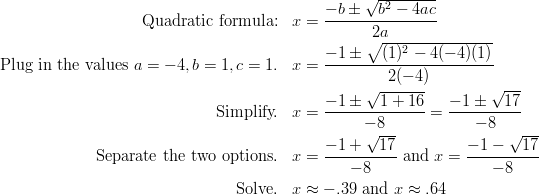
The solution to any quadratic equation in standard form ![]() is
is
![]()
Example: Solve ![]() using the Quadratic Formula.
using the Quadratic Formula.
Solution: We know from the last lesson the answers are ![]() or
or ![]() .
.
By applying the Quadratic Formula and ![]() , and
, and ![]() , we get:
, we get:
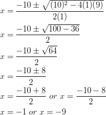
Example 1: Solve ![]() using the Quadratic Formula.
using the Quadratic Formula.
Solution:
Multimedia Link For more examples of solving quadratic equations using the Quadratic Formula, see Khan Academy Equation Part 2 (9:14).

2 more examples of solving equations using the quadratic equation (Click here to watch the video)
Figure 2 provides more examples of solving equations using the quadratic equation. This video is not necessarily different from the examples above, but it does help reinforce the procedure of using the Quadratic Formula to solve equations.
The ![]() coordinate of the vertex of
coordinate of the vertex of ![]() is
is ![]()
Usually you will not be told which method to use. You will have to make that decision yourself. However, here are some guidelines to which methods are better in different situations.
Example: The length of a rectangular pool is 10 meters more than its width. The area of the pool is 875 square meters. Find the dimensions of the pool.
Solution: Begin by drawing a sketch. The formula for the area of a rectangle is ![]() .
.

![]()
Now solve for ![]() using any method you prefer.
using any method you prefer.
The result is ![]() . So, the length of the pool is 35 meters and the width is 25 meters.
. So, the length of the pool is 35 meters and the width is 25 meters.
The following video will guide you through a proof of the Quadratic Formula. CK-12 Basic Algebra: Proof of Quadratic Formula (7:44)
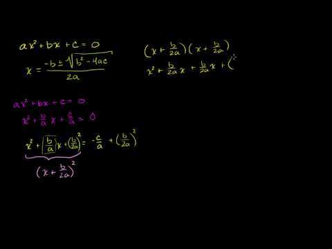
Proof of Quadratic Formula (Click here to watch the video)
Sample explanations for some of the practice exercises below are available by viewing the following video. Note that there is not always a match between the number of the practice exercise in the video and the number of the practice exercise listed in the following exercise set. However, the practice exercise is the same in both. CK-12 Basic Algebra: Using the Quadratic Formula (16:32)

Using the Quadratic Formula (Click here to watch the video)
Find the ![]() coordinate of the vertex of the following equations.
coordinate of the vertex of the following equations.
Solve the following quadratic equations using the Quadratic Formula.
Solve the following quadratic equations using the method of your choice.


Mixed Review
You have seen parabolas that intersect the ![]() axis twice, once, or not at all. There is a relationship between the number of real
axis twice, once, or not at all. There is a relationship between the number of real ![]() intercepts and the Quadratic Formula.
intercepts and the Quadratic Formula.
Case 1: The parabola has two ![]() intercepts. This situation has two possible solutions for
intercepts. This situation has two possible solutions for ![]() , because the value inside the square root is positive. Using the Quadratic Formula, the solutions are
, because the value inside the square root is positive. Using the Quadratic Formula, the solutions are ![]() and
and ![]() .
.

Case 2: The parabola has one ![]() intercept. This situation occurs when the vertex of the parabola just touches the
intercept. This situation occurs when the vertex of the parabola just touches the ![]() axis. This is called a repeated root, or double root. The value inside the square root is zero. Using the Quadratic Formula, the solution is
axis. This is called a repeated root, or double root. The value inside the square root is zero. Using the Quadratic Formula, the solution is ![]() .
.

Case 3: The parabola has no ![]() intercept. This situation occurs when the parabola does not cross the
intercept. This situation occurs when the parabola does not cross the ![]() axis. The value inside the square root is negative, therefore there are no real roots. The solutions to this type of situation are imaginary, which you will learn more about in a later textbook.
axis. The value inside the square root is negative, therefore there are no real roots. The solutions to this type of situation are imaginary, which you will learn more about in a later textbook.

The value inside the square root of the Quadratic Formula is called the discriminant. It is symbolized by ![]() . It dictates the number of real solutions the quadratic equation has. This can be summarized with the Discriminant Theorem.
. It dictates the number of real solutions the quadratic equation has. This can be summarized with the Discriminant Theorem.
Example 1: Determine the number of real solutions to ![]() .
.
Solution: By finding the value of its discriminant, you can determine the number of ![]() intercepts the parabola has and thus the number of real solutions.
intercepts the parabola has and thus the number of real solutions.

Because the discriminant is positive, the parabola has two real ![]() intercepts and thus two real solutions.
intercepts and thus two real solutions.
Example: Determine the number of solutions to ![]() .
.
Solution: Before we can find its discriminant, we must write the equation in standard form ![]() .
.
Subtract 4 from each side of the equation: ![]() .
.
![]()
The value of the discriminant is negative; there are no real solutions to this quadratic equation. The parabola does not cross the ![]() axis.
axis.
Example 2: Emma and Bradon own a factory that produces bike helmets. Their accountant says that their profit per year is given by the function ![]() , where
, where ![]() represents the number of helmets produced. Their goal is to make a profit of $40,000 this year. Is this possible?
represents the number of helmets produced. Their goal is to make a profit of $40,000 this year. Is this possible?
Solution: The equation we are using is ![]() . By finding the value of its discriminant, you can determine if the profit is possible.
. By finding the value of its discriminant, you can determine if the profit is possible.
Begin by writing this equation in standard form:

Because the discriminant is positive, the parabola has two real solutions. Yes, the profit of $40,000 is possible.
Multimedia Link: This http://sciencestage.com/v/20592/a-level-maths-:-roots-of-a-quadratic-equation-:-discriminant-:-examsolutions.html - video, presented by Science Stage, helps further explain the discriminant using the Quadratic Formula.
Sample explanations for some of the practice exercises below are available by viewing the following video. Note that there is not always a match between the number of the practice exercise in the video and the number of the practice exercise listed in the following exercise set. However, the practice exercise is the same in both. CK-12 Basic Algebra: Discriminant of Quadratic Equations (10:14)
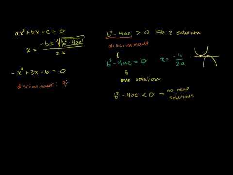
Discriminant of Quadratic Equations (Click here to watch the video)
Find the discriminant of each quadratic equation.
Determine the nature of the solutions of each quadratic equation.
A solution to a quadratic equation will be irrational if the discriminant is not a perfect square. If the discriminant is a perfect square, then the solutions will be rational numbers. Using the discriminant, determine whether the solutions will be rational or irrational.
Mixed Review
 .
.
So far in this text you have learned how to graph three very important types of equations.
In real-world applications, the function that describes some physical situation is not given. Finding the function is an important part of solving problems. For example, scientific data such as observations of planetary motion are often collected as a set of measurements given in a table. One job for the scientist is to figure out which function best fits the data. In this lesson, you will learn some methods that are used to identify which function describes the relationship between the dependent and independent variables in a problem.
By finding the differences between the dependent values, we can determine the degree of the model for the data.

Example: The first difference is the same value (3). This data can be modeled using a linear regression line.
The equation to represent this data is ![]()
When we look at the difference of the ![]() values, we must make sure that we examine entries for which the
values, we must make sure that we examine entries for which the ![]() values increase by the same amount.
values increase by the same amount.
For example, examine the values in the following table.
At first glance, this function might not look linear because the difference in the ![]() values is not always the same.
values is not always the same.

However, we see that the difference in ![]() values is 5 when we increase the
values is 5 when we increase the ![]() values by 1, and it is 10 when we increase the
values by 1, and it is 10 when we increase the ![]() values by 2. This means that the difference in
values by 2. This means that the difference in ![]() values is always 5 when we increase the
values is always 5 when we increase the ![]() values by 1. Therefore, the function is linear.
values by 1. Therefore, the function is linear.
The equation is modeled by ![]() .
.
An example of a quadratic model would have the following look when taking the second difference.

Finding the difference involves subtracting the dependent values leading to a degree of the model. By taking the ratio of the values, one can obtain whether the model is exponential.
If the ratio of dependent values is the same, then the data is modeled by an exponential equation, as in the example below.

To enter data into your graphing calculator, find the [STAT] button. Choose [EDIT].


Enter the data into the appropriate list. Using the first set of data to illustrate yields:

You already know this data is best modeled by a linear regression line. Using the [CALCULATE] menu of your calculator, find the linear regression line, linreg.


Look at the screen above. This is where you can find the quadratic regression line [QUADREG], the cubic regression line [CUBICREG], and the exponential regression line, [EXPREG].
Sample explanations for some of the practice exercises below are available by viewing the following video. Note that there is not always a match between the number of the practice exercise in the video and the number of the practice exercise listed in the following exercise set. However, the practice exercise is the same in both. CK-12 Basic Algebra: Linear, Quadratic, and Exponential Models (8:15)

Linear, Quadratic, and Exponential Models (Click here to watch the video)
Determine whether the data can be modeled by a linear equation, a quadratic equation, or neither.
Can the following data be modeled with an exponential function?
Determine whether the data is best represented by a quadratic, linear, or exponential function. Find the function that best models the data.
| Time (seconds) | Height (inches) |
| 2 | 2 |
| 2.2 | 16 |
| 2.4 | 24 |
| 2.6 | 33 |
| 2.8 | 38 |
| 3.0 | 42 |
| 3.2 | 36 |
| 3.4 | 30 |
| 3.6 | 28 |
| 3.8 | 14 |
| 4.0 | 6 |
| Day | Weight(grams) |
| 0 | 250 |
| 1 | 208 |
| 2 | 158 |
| 3 | 130 |
| 4 | 102 |
| 5 | 80 |
| 6 | 65 |
| 7 | 50 |
| Year | Rate of Pregnancy (per 1000) |
| 1990 | 116.9 |
| 1991 | 115.3 |
| 1992 | 111.0 |
| 1993 | 108.0 |
| 1994 | 104.6 |
| 1995 | 99.6 |
| 1996 | 95.6 |
| 1997 | 91.4 |
| 1998 | 88.7 |
| 1999 | 85.7 |
| 2000 | 83.6 |
| 2001 | 79.5 |
| 2002 | 75.4 |
Mixed Review
As you learn more and more mathematical methods and skills, it is important to think about the purpose of mathematics and how it works as part of a bigger picture. Mathematics is used to solve problems that often arise from real-life situations. Mathematical modeling is a process by which we start with a real-life situation and arrive at a quantitative solution.
Modeling involves creating a set of mathematical equations that describes a situation, solving those equations, and using them to understand the real-life problem.
Often the model needs to be adjusted because it does not describe the situation as well as we wish.
A mathematical model can be used to gain understanding of a real-life situation by learning how the system works, which variables are important in the system, and how they are related to each other. Models can also be used to predict and forecast what a system will do in the future or for different values of a parameter. Lastly, a model can be used to estimate quantities that are difficult to evaluate exactly.
Mathematical models are like other types of models. The goal is not to produce an exact copy of the “real” object but rather to give a representation of some aspect of the real thing. The modeling process can be summarized as a flow chart:

Notice that the modeling process is very similar to the problem-solving format we have been using throughout this book. One of the most difficult parts of the modeling process is determining which function best describes a situation. We often find that the function we choose is not appropriate. Then we must choose a different one.
Consider an experiment regarding the elasticity of a spring.
Example: A spring is stretched as you attach more weight at its bottom. The following table shows the length of the spring in inches for different weights in ounces.
![]()
a) Find the length of the spring as a function of the weight attached to it.
b) Find the length of the spring when you attach 5 ounces.
c) Find the length of the spring when you attach 19 ounces.
Solution: Begin by graphing the data to get a visual of what the model may look like.

Example: A golf ball is hit down a straight fairway. The following table shows the height of the ball with respect to time. The ball is hit at an angle of ![]() with the horizontal with a speed of 40 meters/sec.
with the horizontal with a speed of 40 meters/sec.
![]()
a) Find the height of the ball as a function of time.
b) Find the height of the ball when ![]() .
.
c) Find the height of the ball when ![]() .
.

Solution: Begin by graphing the data to visualize the model.
This data fits a parabolic curve quite well. We can therefore conclude the best model for this data is a quadratic equation.
To solve part a), use the graphing calculator to determine the quadratic regression line.
![]()
b) The height of the ball when ![]() is:
is:
![]()
c) The height of the ball when ![]() is
is
![]()
Sample explanations for some of the practice exercises below are available by viewing the following videos. Note that there is not always a match between the number of the practice exercise in the videos and the number of the practice exercise listed in the following exercise set. However, the practice exercise is the same in both.
CK-12 Basic Algebra: Identifying Quadratic Models (8:05)
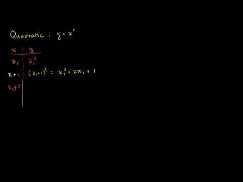
Using y=x^2 to give a sense of why the change in the change of y (or the change in the slope) is constant (Click here to watch the video)
CK-12 Basic Algebra: Identifying Exponential Models (4:00)

Identifying Exponential Models (Click here to watch the video)
CK-12 Basic Algebra: Quadratic Regression (9:17)

Using a calculator to perform a quadratic regression (Click here to watch the video)
![]()
generation.
![]()
Mixed Review
form.
Define each term.
Graph each function. List the vertex (round to the nearest tenth, if possible) and the range of the function.
Rewrite in standard form.
Solve each equation by graphing.
Solve each equation by taking its square roots.
Solve each equation by completing the square then taking its square roots.
Determine the maximum/minimum point by completing the square.
Solve each equation by using the Quadratic Formula.
In 45-50, for each quadratic equation, determine:
(a) the discriminant
(b) the number of real solutions
(c) whether the real solutions are rational or irrational
![]()
years.
![]()
years.
![]()
table.
![]()
In 5–9, solve the equation using any method.
| Year | Number of Deaths Per 100,000 men |
| 1980 | 205.3 |
| 1985 | 212.6 |
| 1989 | 217.6 |
| 1993 | 212.1 |
| 1997 | 201.9 |
In the CK-12 Texas Instruments Algebra I FlexBook, there are graphing calculator activities designed to supplement the objectives for some of the lessons in this chapter. See http://www.ck12.org/flexr/chapter/9620.