1 Introduction
The evolution of the communications and the Internet have allowed the integration of different kind of services and infrastructures. From the active web pages, passing through the social networks and mobile devices to the real-time data consuming, they are today the current coin in a world dominated by the communication and the information systems [1]. In this context, the data are continuously generated under different kinds of formats and following a specific underlying model.
Nowell, along with the data generation process, it is possible to differentiate at least between the real-time data and historical data. On the one hand, the real-time data are consumed as close as possible to the generation instant, and the life cycle is limited to the arrival of new data (i.e. the new data implies the substitution and updating of the previous data, allowing describing an updated situation). On the other hand, the historical data are consumed at any moment and they are oriented to characterize a given historical situation, conceptualizing the idea of “historical” such as a captured past event in relation to the current time (e.g. the past five minutes). The real-time and historical data are useful in its own context, that is to say, the real-time data are mainly oriented to the active monitoring of an entity under analysis (e.g. an outpatient, the environment, etc.), while the historical data are associated with the non-critical information systems in where there exists tolerance in relation to the answer time and its processing.
In this sense, the data source is understood such as an integrable component (physical or not) with a given precision and accuracy, able to generate data under a particular organization from a given entity. The entity represents any concept able to be analyzed through a set of measurable characteristics (be abstract characteristics or not). Thus, the idea of data source could be matched with different kinds of physical sensors, or even a software measuring specific aspects of other software.
The configuration possibilities associated with each data source are very wide and it depends on the specific application, and for that reason, the likelihood to find heterogeneous data sources is very high. For example, it could be possible to measure the water temperature using a digital thermometer, or by mean of a thermometer based on mercury. In both cases, the measured value could be similar, however, the data organization for informing the current data, the accuracy and precision could be different.
Another important aspect in relation to the data sources is its autonomy, that is to say, each data source sends the captured and observed data from its own entity under analysis, and no one external entity could affect or interrupt its internal behavior. Continuing the example of the water temperature, the thermometer informs the value of the measured temperature from the water following a given technique, but this is independent of other devices. This is important to highlight because a data processor is not able to affect or modify the expected behavior from the data sources, it just can receive and process the sent data from the data source.
Thus, the basic idea of data source could be defined as an integrable component, heterogeneous, with a given precision and accuracy, susceptible to be calibrated, autonomous in terms of the measurement technique and the measure production, with basic interaction capacities limited to the coordinating of the data sending.
The evolution of the data sources converges today in the idea associated with the Internet of Thing [2]. Before defining it, it is important to say that by “things” is understood that data source able to interact by wireless connections with other devices, conforming, integrating or scaling new services. Thus, the Internet of Thing could be defined such as the autonomous capacity related to a set of pervasive “things” connected through wirelesses, which is able to integrate, extend or support new kind of services by mean of the interaction among them. In this kind of environment, the things could be heterogeneous, and for that reason, the data interchanging requires a common understanding which fosters the interoperability from the syntactic and semantic point of view.
In this way, the data could be continuously generated from different environments and any time, which implies a rapid growing of the volume and variety of data. In the case of the data should be stored, it gives place to a big data repository. In effect, the three Big Data V’s implies velocity, variety, and volume. The volume of data is associated with the huge of collected data from the devices which must be permanently stored. The variety refers to the kind of data to be stored, queried and processed coming from the devices (e.g. a picture, information geographic, etc.). Finally, the velocity refers to the growth projection of the Big Data repository in relation to the incoming data.
The Big Data repositories could be as big as possible, but they are finite. That is to say, they may incorporate a lot of data, but always the volume is quantifiable and determined. The last is a key difference in relation to the real-time data collecting and processing, because, for example, the sensors are permanently sending data, the data are useful at the generation instant and the volume of the data just could be estimated but not determined.
In other words, the size of a Big Data repository could be computed, but the size of a data flow is not limited. This is a key difference between the Big Data and the real-time data processing approach. For example, it supposes that a user needs to match their customers with its geographic information for putting the customer information on a map. Both the customer and the information geographic corresponds with a finite set, with a given size, in where the sets could be analyzed and processed for obtaining the wished results. The results can be ordered in absolute terms because the result set is finite too. However, if the user wants to merge the share prices from New York with Tokyo for a given stock, the resulting is continuously updated with each new data and the final size is not determined. Even, the order in which the resulting could be sent to the user is relative because such order is limited to the currently processed data.
1.1 The Data Stream Environment
One of the main aspects to consider in this new communicated world is the usefulness of the data stream and what is the advantage in relation to the persistent data strategy. In this sense, it is necessary to say that the stored data are inadequate when the data is oriented to the active monitoring. That is to say, the time for the data retrieving from a persistent device is upper than the required time for processing them at the moment in which they arrive. The idea of the data stream is associated with the data processing exactly when they have arrived. Thus, they are ideally read one time, because a new reading would simply lose the opportunity to read the new data.
The data stream could be defined in terms of Chaudhry [3] such as an unbounded data sequence. In addition, it is important to incorporate that the data sequence could have a data organization and the order in each sequence is relative only to a given sequence. For this reason, the definition could be updated and extended saying that the data stream is an unbounded data sequence in where the data could be structured under a given data model and the order of each datum is relative to its own sequence.
The real-time data and its associated processing, present key differences in relation to the data stored in a Big Data repository, which can be synthesized in at least three: time notion, reliability, and reaction. In the data stream, the data are processed at the moment in which they arrive, they push the old data (updating them), and the data are processed as they are, be reliable or not. Even, the data stream incorporates the notion of time in its own generation chronology. However, a Big Data repository does not necessarily incorporate the notion of time, the data must be queried, and because they are able to be analyzed and controlled, they have an upper level of reliability.
The arriving: The data elements arrive in a continuous way, keeping a relative order to the sequence itself,
The notion of time: The idea of time is incorporated, be in the underlying data model or in the sequence,
The Data Origin: The data source is associated with the data stream (e.g. a temperature sensor), that is to say, the data origin is unmodifiable by any data processor,
The input from the data stream: It is unpredictable in terms of rate or volume of data,
The Data Model: Each data stream could have its own underlying data model or not (e.g. it could be semi-structured such as an XML document, or not structured like a text file),
Data Reliability: The data inside of the data stream are processed like they are, they are not free of errors because depend on the data source and the transited path,
For boarding the data stream processing, the idea of “window” was proposed. Basically, a window is a logical concept associated with some kind of partition of the original data stream for making easier the partial data processing. Synthetically, it is possible to define a window in terms of a given magnitude of time (physical window), for example, the window keeps the data related to ten minutes. In addition, it is possible to define a window in terms of a given quantity of data (logical window), for example, one hundred messages from the data source. Nowell, when the logical or physical window implies to keep static the width and update its content based on a notion of time (the new data replace to the old data), the window is known as a sliding window. For example, the last five minutes (sliding physical window), the last one hundred messages (sliding logical window), etc.
1.2 The Big Data Environment
The Big Data is a term which describes a huge of data, following a data model, which continuously overflow with data to the organization. The processing strategy is thought for batch processing, fostering the parallelization strategy, on the base on a given requesting (On-demand).
As it was introduced before, the original three “V” of the Big Data is associated with variety, volume, and velocity. The variety implies that the data contained inside the repositories are associated with different kinds (e.g. associative, relational, audio, etc.). The volume refers to the huge of data available in the repository for processing and analysis. The Velocity concept is associated with the increasing rate of the data in relation to the repository and its sizing.
Even more, the variability of the provided data is a current concern in the discipline, because the data coming from independent data sources (such as the data streams) could incorporate inconsistent data in the repository. In addition, the processing complexity is incremented from the heterogeneity of the underlying data models and the diversity of kind of data.
An additional “V” was proposed in relation to the value of the data and its importance for the decision-making process. That is to say, the idea of value refers to the capacity of obtaining new information through some kind of processing from the stored data in a repository. This gives a start to the idea of data monetization, in other words, the way to make money by using the data available on the repository [5].
However, the four mentioned “V” are not the only “V” because Khan et al. [6] proposed another “V” as complement, such as (i) Veracity: it refers to the trust respect the data when it needs to be used for supporting the decision making, (ii) Viscosity: it is associated with the level of relationship among complex data (cohesion and dependence), (iii) Variability: it is related to the inconsistent data flow which takes a special interest in the measurement projects, (iv) Volatility: it is associated with the data lifecycle and its necessity of being stored, (v) Viability: it is related which the time where the data is useful for generating new information, and (vi) Validity: It refers to the fitted and compatible data for a given application.
The idea associated with the NoSQL database simply refers to “Not only SQL” in relation to the databases. That is to say, the NoSQL databases are oriented to implement a different data model to the relational data model. There are at least four basic NoSQL data model related to the Big Data repositories [7]: (i) The Wide-Column Data Model: the data are organized in terms of tables, but the columns become to a column family, being it fully dynamic aspect. The atomicity principle is not applied here such as the relational model, and for that reason the content is heterogeneous. Even, the structure between rows (e.g. the quantity of columns) is not necessarily the same. (ii) The Key-Value Data Model: It looks like a big hash table where the key allows identifying a position which contains a given value. The value is a byte flow, and for that reason, it represents anything expressible like byte stream (e.g. picture, video, etc.), (iii) The Graph Data Model: each node represents a data unit, and the arcs with a given sense implement the relationships among them, and (iv) Document-oriented Data Model: The data are hierarchically organized, and they are free of a schema. Each stored value is associated with a given key, being possible to store the data formats such as JSON, XML, among others.
Because the uses and applications of the NoSQL databases do not necessarily have a transactional target [8], the ACID (Atomicity, Consistency, Isolation, and Durability) principle is not critical or mandatory to consider. Thus, the BASE (Basically Available, Soft State, and Eventually Consistent) principle is better fitted in NoSQL databases [9]. In this sense, basically available implies that the answer is guaranteed even when the data are obsolete. The Soft State refers to the data are always available for receiving any kind of changing or updating. Finally, eventually consistent implies that given the distributed nature of the nodes, the global data as a unit will be in some instant consistent.
Even when the data stream and the Big Data environment have different kinds of requirements in terms of the available resources, data organization, processing strategy and, data analysis, they could be complementary. That is to say, in case of having that to store a data representative quantity from a data stream, the ideal kind of repository for managing a massive dump of data is precisely a Big Data repository because allows keeping the stability and scalability at the same time.
1.3 Main Contributions
As contributions of this chapter: (i) An Integrated and Interdisciplinary View of the Data Processing in the Heterogeneous Contexts is presented: An integrated perspective under the figure of a processing architecture based on measurement metadata, which includes from the heterogeneous data sources (e.g. Internet of things) to the real-time decision making based on the recommendations (i.e. knowledge and previous experiences). The fully-updated main processes are detailed using the Business Process Model and Notation (BPMN)1; (ii) The integration between the measurement and evaluation framework and the real-time processing is detailed: In a data-driven decision-making context, the concept monitoring and the real-time data processing are a key aspect. In this sense, the importance of the measurement and evaluation project definition in relation to the data processing (be it online or batch) is introduced and exemplified; (iii) The Interoperability as the axis of the Processing Architecture: Because of the data sources are heterogeneous, the Measurement Interchange Schema (MIS) is introduced jointly with its associated library, as a strategy for the data integration of different kinds of devices. Even, the project definition schema based on the measurement and evaluation framework is highlighted in terms of its importance for the interoperability among the different measurement systems; and (iv) The similarity as a recommending strategy improves the decision-making support: Because of some monitored concept could do not have previous experiences or knowledge, a strategy oriented to the similarity-based searching is proposed for the organizational memory. Thus, the idea is found the experiences as close as possible to a given situation for a complementary recommending. This allows a better support to the decision-making process in presence of the uncertainty.
1.4 An Outline of the Rest of the Chapter
Thus, having introduced important aspects related to the Big Data Repositories and NoSQL databases, jointly with the underlying concepts to the data streams and the Internet of Thing, in the following sections an overview of the proposal for the integral boarding of the real-time monitoring applied in the measurement and evaluation area is synthesized. Section 2 presents a synthesis associated with the data stream management system. Section 3 describes the basic steps for defining a measurement and evaluation project. Section 4 introduces the measurement interchange schema. Section 5 outlines the Processing Architecture based on Measurement Metadata. Section 6 describes the main processes related to the Processing Architecture in terms of the Business Process Model and Notation (BPMN). Section 7 introduces an application case for an integral boarding of the measurement and evaluation project. Section 8 outlines some related works. Finally, Sect. 9 presents some conclusions and future trends related to the area.
2 The Data Stream Management System
The Data Stream Processing (DSP) could be viewed as a programming paradigm oriented to the transformation or change in any form of the data continuously arriving through one or more data sources [10]. Returning to the concept of data stream introduced before, the data stream is an unbounded data sequence in where the data could be structured under a given data model and the order of each datum is relative to its own sequence. Thus, the Data Stream Management System (DSMS) could be defined as the software responsible for the implementing of the data stream processing, considering from the data sources, the data transformation to the output managing.
Each operation applied to a given data on a data stream is defined through an operator which is able to transform, change and/or replicate in any form the data stream. The operations applied to the data stream can be pipelined following a given order defined by an application. This pipeline allows connecting the operations and their results with the aim of building a global pipelining system of data, connecting each data source with the expected outputs. Thus, the data stream applications exploit the parallelism given by the pipelines, taking advantage of the common hardware for scalability and the infrastructure economy [11].

The architectural view of the data stream management system
The stream and query catalog (see Fig. 1, on the left lower angle) is basically responsible for: (i) The data stream structure definition: It is associated with the structural definition of each data stream to be consumed by the stream receiver; (ii) The data stream statistics: It represents the collecting of the arrival rate, data volume, among others aspects necessaries for the query planner and the managing of each data stream; (iii) The data stream validity: It defines the data stream to be accepted along with a given time period; (iv) The data stream prioritization: It establishes the prioritization to be considered for the data stream receiving and processing in case of the resources are committed; (v) The operation definition: It is responsible for defining the inputs, the transformation or associated procedure jointly with the expected operation outputs; (vi) Pipelines definition: It establishes the way in which the operations and data streams are connected, and (vii) Query Catalog: It registers the set of the planned queries for the data streams or intermediate results.
The Monitoring and Planning Engine (see Fig. 1, on the middle lower region) is responsible for: (i) The resources monitoring: The main responsibility is the real-time monitoring associated with the pipelines, planned queries and ad hoc queries. This allows warrantying enough resources for generating the expected outputs; (ii) The Service Queue Manager: It is responsible for the ordering of the operations in the runtime environment, considering the available resources; (iii) The query planner: From the statistics related to the data streams, the available resources, and the associated definitions, it is responsible for the organization of the query plan and its communication to the service queue manager; (iv) The performing coordinator: From the real-time information provided by the resource monitoring and the query planner, it is responsible for launching and warrantying the running of each operation from the beginning to the end.
The Persistence Manager (see Fig. 1, on the right lower angle) is responsible for the storing of the data following the indicated synthesis strategy, but just when it is required. That is to say, this component is optional and could be out of the bundle of a given data stream management system. When the persistence manager is incorporated as component inside the data stream management system, the main responsibilities are associated with: (i) The synthesis services: it describes the strategy for identifying the data to be kept in a persistent way from the real-time data stream, (ii) The storage services: It is responsible for establishing the necessary channels for storing and retrieving the data from the external storage unit; and (iii) The historical data services: This service is responsible for the query plan optimization, retrieving, and the output organization from a given external query on the historical data.
Thus, the Stream Receiver (see Fig. 1, on the left upper angle) is who determines whether a data stream is accepted or not, using the defined metadata in the data stream catalog. In this sense, a data stream could be correctly defined, but its life period is not valid (e.g. it has expired). All the defined data streams with a valid time period are monitored for collecting statistics. The statistics are sent for its posterior use in the planners (e.g. the query planner). Once the statistics were collected, the data streams pass through a load shedder. The load shedder discards in a selective way the data, keeping those considered as important in base on its definition. The use of the load shedding techniques is optional, and they are applicable when the available resources are near to the maximum limit. Once the data stream has got out from the load shedder, the output could directly go to an operation, or well, it could be used in a planned query. In the case of a planned query, the output could be directly sent to the output manager or even to another operation.
The processor (see Fig. 1, on the middle upper region) is who keep flowing the data from the data stream, passing through the operations to the output manager [12, 13]. It is responsible for the real-time computing, implementing of the pipelines, data transformation, and the communication of the results to the output manager. An interesting thing incorporated on each operation is the idea of the synopsis. The synopsis is an in-memory materialized operation result who kept the last known result for the associated operation. This materialized result is useful for continuing the processing with the posterior operations, even when the inputs of the origin operation were interrupted.
The Output Manager (see Fig. 1, on the right upper angle) regulates the way in which the outputs are communicated jointly with its monitoring (e.g. the output rate). The output (i.e. the result associated with a pipeline, planned query or ad hoc query) could be replicated to other sites or systems, but also, it could be directly consumed by mean of a set of users or systems. In this sense and on the one hand, the replication service is responsible for automatically serving the outputs to the configured systems or users. On the other hand, the subscription service regulates the target associated with the consumers of each stream and the valid life cycle in which they could consume each output.
The Internet of Thing, Data Streams, Big Data and Data Stream Management Systems are converging in application joint areas, such as the healthcare [14] among other areas. That is to say, the Internet of Thing (IoT) allows boarding the data collection with different kind of devices, communicating they between them and transmitting different kinds of data (e.g. from information geographic to pictures). On the one hand, the collected data from the different “Things” could be stored in case of necessity, which considering that the data streams are potentially unbounded will give origin to a Big Data Repository. On the other hand, when the data coming from the “Things” should be processed when they arrive, it is necessary for the incorporation of the DSMS. Thus, The IoT, Big Data and the DSMS allow the implementing of the measurement process as a strategy for knowing and monitoring the current state of some concept under interest [15].
3 The Measurement and Evaluation Project Definition
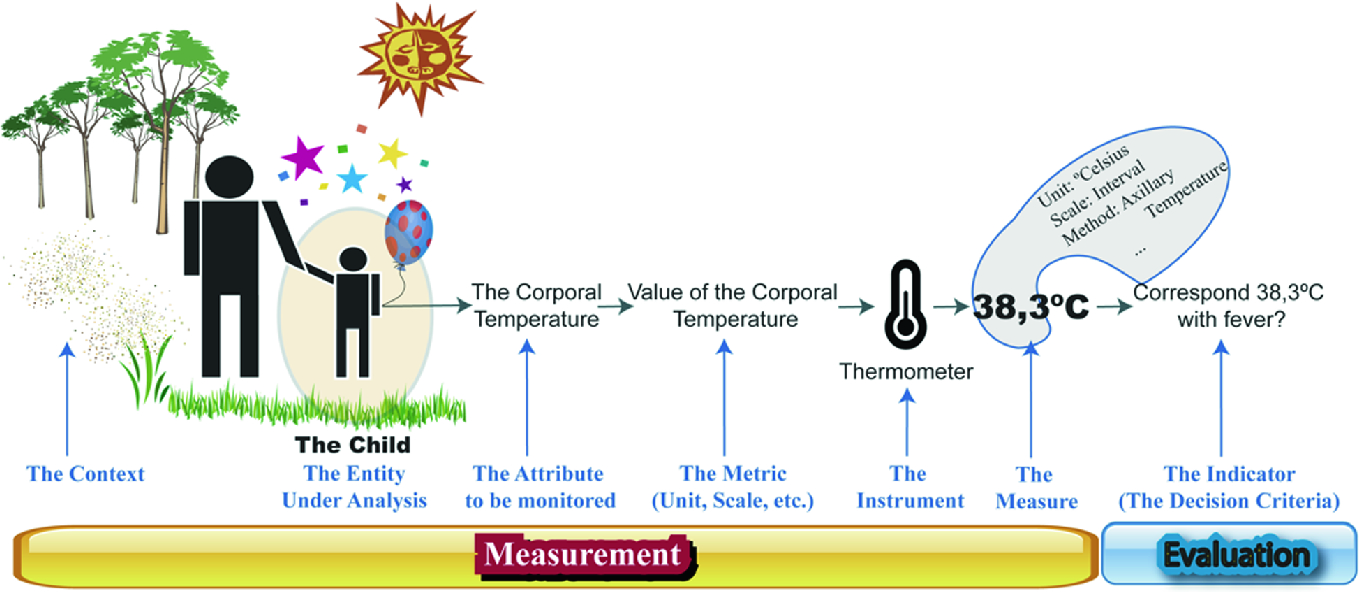
The way in which the person naturally knows the state or situation of an object is through the measurement, for example, when a child goes to the periodical medical visit, the doctor checks its size, height, weight, among other aspects comparing all of them with the previous medical visit. In this sense, measuring and comparing the current and past values, the doctor could determine its evolution. Even when this could seem to be as an elemental thing, the measurement involves a set of details which are critical at the time in that the values should be obtained, compared and evaluated.
A conceptual view of the measurement process
The measurement process is a key asset for reaching a predictable performance in the processes, and it incorporates the assumptions of the repeatability, comparability of the results, and extensibility [16]. That is to say, (i) the repeatability is the possibility of applying in an autonomous and successive way the same measurement process, independently of the person/machine responsible for the application itself; (ii) the comparability of the results implies that the values are homogeneous and obtained following the same method and using compatible instruments for its implementing; and (iii) the extensibility refers to the possibility of extending the measurement process when there are new requirements.
The measurement and evaluation frameworks allow defining the measurement process with the aim of guarantying the repeatability of the process, the comparability of the associated results and its extensibility when there are new requirements [17]. There are many examples from traditional approaches such as The Goal-Question-Metric paradigm [18], passing through the C-INCAMI (acronym for Context-Information Need, Concept Model, Attribute, Metric, and Indicator) [19, 20] framework, to most recent approach such as the “Agg-Evict” framework [17] oriented to the network measurement.
Thus, the repeatability of the measurement process implies a common understanding related to the underlying concepts (e.g. metric, measure, assessment, etc.), which is essential for its automatization, for example, through the IoT as the data collectors and the DSMS as the data processor.
The idea of estimated and deterministic measure,
The incorporation of the complementary data related to each measure. The complementary data could be a picture, video, audio, plain text, and/or information geographic,
The managing of the data sources and the associated constraints,
The organization and use of the measurement adapter,
Diverse ways to check the content integrity (e.g. be it at message or measure level), and
The possibility of carrying forward the data traceability,
The C-INCAMI framework is guided by an information need, which allows establishing the entity under analysis and describing the attributes who characterize it. Each attribute is associated with a metric, who is responsible for its quantification. The metric defines the method, scale, unit, the associated instrument (i.e. the data source) among other aspects for obtaining and comparing the measure. Each metric could obtain a set of measures. The measure represents a specific value obtained by mean of the metric, at a specific time. The measure alone does not say much, but the role of the indicator allows interpreting each measure through the incorporation of the decision criteria. For example, given a temperature obtained from a metric, the indicator (through the decision criteria) allows knowing whether a child suffers fever or not (see Fig. 2).
The way in which a measurement and evaluation project could be formally defined using the C-INCAMI framework is defined in [22], and just a few basic steps are requested: (i) The definition of the non-functional requirements: it is responsible for establishing the information need related to the project and the identification of the entity category (e.g. a lagoon, a person, etc.), the entity to monitor (e.g. John Doe) and the attributes for quantifying it; (ii) Designing the Measurement: Once the entity is defined and their attributes identified, the metric is defined for each attribute jointly with its association with the data source (e.g. a given sensor in IoT); (iii) Implementing of the Measurement: The measurement is effectively activated through the different sensors associated with each metric and the measures start to arrive for its processing; (iv) Designing the Evaluation: The indicators and the associated decision criteria are defined for interpreting each measure from the metrics; (v) Implementing of the Evaluation: The indicators, decision criteria, and the decision-making is effectively put to work through an automatized process; and (vi) Analyzing and Recommending: It is responsible for analyzing each decision from the indicators and to give some recommendations pertinent to the configured situation.
The “Bajo Giuliani” is a lagoon located around 10 km at the south of the Santa Rosa city, province of La Pampa in Argentina (South-America). On the south shore of the lagoon, there is a neighborhood named “La Cuesta del Sur”. This lagoon receives water from the raining and waterways coming from the city. On the lagoon, the national route number 35 cross it from the north to south. For clarifying the idea associated with the project definition, the basic steps are exemplified. Thus, the project’s information need could be defined as “Monitor the level of water of the ‘Bajo Giuliani’ lagoon for avoiding flood on the south shore related to the neighborhood”. The entity category is defined such as “lagoon located in the province of La Pampa”, principally considering the particularities of this region and the semi-arid climate. The entity under analysis or monitoring is limited to the “Bajo Giuliani” lagoon. Nowell, the attributes to choose should characterize the lagoon in relation to the defined information need. For that reason, it is chosen: (i) The water temperature: It allows determining the possibilities of the evaporation in relation to the lagoon; (ii) The ground moisture: it facilitates identifies the regions in which the water advance on the south shore and the regions in which the water is retreating; and (iii) The water level: It allows determining the variation of the water level between the floor of the national route number 35 (it is crossing the lagoon) and the south shore floor related to the neighborhood. In relation to the context, the environmental temperature and humidity are considered for analyzing the effect of the evaporation and the risk of fog on the national route respectively. Even, a picture would be a good idea like complementary datum, principally considering the aspects related to the fog, evaporation, and the environmental temperature.
It is important to highlight that the number of attributes for describing to an entity under analysis jointly with the number of the context properties for characterizing the related context is arbitrarily defined by the analyst responsible for the measurement process. In this case and following the principle of parsimony, these attributes and context properties are kept for exemplifying the idea and the associated applications along this chapter.
Once the attributes and context properties are known and clearly limited, the definition of each metric associated with them is necessary for its quantification. In this sense, the definition of each metric allows specifying the ID associated with the metric, the kind of metric, the associated scale (i.e. kind of scale, the domain of values and the unit), and the associated method. The method describes its name (this is important when it is standardized), the kind of measurement method (i.e. objective or not), a brief narrative specification and the instrument to be used for effectively getting the measure (or value). This step is critical because here it is possible to define whether the expected measure will be deterministic or not.
An example of the definition for the metric related to the water temperature attribute
Metric | ID: 1 Name: value of the water temperature |
Kind | Direct metric |
Scale | • Kind: Interval • The domain of Values: Numeric, Real • Unit: ºCelsius |
Method | • Name: Submerged by direct contact • Measurement method: objective • Specification: It takes the water temperature in the specific position where the monitoring station based on the Arduino One is located. The water temperature is taken at least around 5 cm under the level of the water surface • Instrument: Sensor Ds18b20 (Waterproof) mounted on the Arduino One board • Kind of values: Deterministic |
An example of the definition for the metric related to the environmental humidity context property
Metric | ID: 2 Name: Value of the environmental humidity |
Kind | Direct metric |
Scale | • Kind: Interval • The domain of Values: Numeric, • Unit: % (Percentage) |
Method | • Name: Direct exposition to the environment • Measurement method: objective • Specification: It takes the environmental humidity in the specific position where the monitoring station based on the Arduino One is located. The environmental humidity is taken at least around 2 m above the level of the floor related to the south shore of the neighborhood • Instrument: The DHT11 humidity sensor mounted on the Arduino one board • Kind of values: Deterministic |

As it is possible to appreciate between Tables 1 and 2, the definition of a metric has no difference whether it is a context property or an attribute, because the context property is really an attribute. However, the context property is conceptually specialized for describing a characteristic of the entity context.
Thus, the defined metrics for the entity attributes and the context properties allows obtaining a value, be it deterministic or not. Nowell, the interpretation of each value is an aspect associated with the indicator definition. In this sense, the conceptual differentiation between metric and indicator is that the metric obtains the value, and the indicator interprets each value from a given metric.
 . The conversion or transformation of the metric value is not mandatory, but many times is used for expressing transformations or for linking a set of metrics. Thus, once the formula value is obtained, the decision criteria incorporate the knowledge from the experts for interpreting each value, and for example, when the value of the environmental humidity is 96%, the decision criterium using the Table 3 will say “Very High” and will indicate a specific action to do. The Kind of answer based on the interpretation is defined as a categoric value and with an ordinal scale limited to the following values “Very High”, “High”, “Normal”, “Regular”, and “Low” in that order. When some interpretation has an associated action, the interpreter is responsible for performing it. It is important to highlight that the action to do is based on the decision criteria defined by the experts in the specific domain, and it is not related to a particular consideration of the interpreter.
An example of the definition for the indicator related to the environmental humidity context property
Indicator | ID: I2 Name: Level of the value of the environmental humidity | ||
Kind/weight | Elementary indicator Weight: 1 | ||
Reference metrics | MetricID2 (i.e. Value of the environmental humidity) | ||
Model | • Kind: Ordinal • Domain of values: • Unit: Not applicable | ||
Formula | =MetricID2 | ||
Decision criteria | Interval | Interpretation | Actions |
[95%; 100%] | Very high | Notify | |
[80%; 95%) | High | Notify | |
[60%; 80%) | Normal | No action | |
[40%; 60%) | Regular | No action | |
[0%; 40%] | Low | No action | |

Following this same mechanic, all the necessary indicators associated with the “Bajo Giuliani lagoon” can be defined. Thus, on the one hand, the measurement is implemented through the definitions of the metrics who are responsible for obtaining the measures (i.e. the values). On the other hand, the evaluation is implemented through the indicators who are responsible for the interpretation of each value from the metric and the guiding of their derived actions.
The CINCAMI/Project Definition (synthetically, CINCAMI/PD) [23] is a schema based on the C-INCAMI extended framework which allows interchanging the definition of the measurement and evaluation project among different systems. It has an open source library available on GitHub2 for generating and reading the definitions, fostering its interoperability along different kind of systems who need to implement the measurement based on the extended C-INCAMI framework.
Thus, before to board the data stream processing based on the measurement metadata, the next section introduces the measurement interchange schema for demonstrating how the measurement stream can be generated based on the project definition.
4 The Measurement Interchange Schema
Once the Measurement and Evaluation Project is defined, the definition is communicated to the data processing systems jointly with the measurement adapter. The measurement adapter is a role associated with the responsibility for translating the raw data coming from the sensors to a given data format. For example, the data are obtained from the sensors mounted on the Arduino One. The Arduino One takes the raw data and transforms them in a message based on the eXtensible Markup Language (XML)3 or JavaScript Object Notation (JSON)4 to be sent to the data processor.
As it was shown before, the measurement and evaluation project definition allow defining the attributes and context properties for an entity, jointly with the associated metrics. Thus, the measurement adapter and the data processor could interpret a given message using the definition.
Nowell, when the measurement adapter receives the project definition, it associates each sensor value with the expected metric, and in this line, the new messages will be organized using the project definition known as the metadata. In the same sense, the data processor will interpret each message coming from the measurement adapter using the same project definition. This is a key asset because both the sender and receiver share a common project definition for fostering the data interoperability.
The Measurement Interchange Schema (MIS) [21] is structured following the underlying concepts, terms and the relationships associated with the extended C-INCAMI framework, and it is also known under the name of CINCAMI/MIS. The schema allows the measurement interchanging using as guide the project definition. Thus, a CINCAMI/MIS message incorporates the data (i.e. the measures) jointly with the metadata (e.g. the identification of a metric for a given measure) which allow guiding the real-time data processing.
4.1 The Details About the Measurement Schema
The Measurement Interchange Schema is hierarchically organized through an XML schema following the concepts, terms, and relationships associated with the measurement and evaluation project definition.

The upper level of the CINCAMI/MIS message
Thus, Fig. 3 outline the highest level related to the measurement interchange schema. The CINCAMI_MIS tag limits the message for a given measurement adapter. That is to say, each set of measures coming from the same measurement adapter at a given time, it will be organized under the same CINCAMI_MIS tag. This tag has two associated attributes, the version refers to the version of the measurement schema used in the message, while the dsAdapterID refers to the unique identification of the measurement adapter which acts as the intermediary between the data sources (i.e. the sensors) and the data processor.
The measures are grouped through the measurementItemSet tag, which contains a set of measurementItem tag. The measurementItem tag represents one measure associated with its contextual information and complementary data. This tag identifies (1) The data source ID (i.e. the dataSourceID tag) which is the identification of the data source that acts as the origin of the measures; (2) The original data format in which the data source provides the measure to the measurement adapter. For example, and using the Table 1, it would be the data format in that the sensor Ds18b20 informs each measure to the Arduino One in which it is mounted; and (3) The footprint allows an integrity verification on the informed measure, considering the measurement itself jointly with the context information. In addition to the measure and the context information, the measurementItem tag allows identifying the entity under monitoring, which is useful in case of the load shedding techniques and data prioritization in the real-time data processing.

The measurement tag in the CINCAMI/MIS message
Under the Measurement tag there exists the description of the quantitative value jointly with the complementary data. The quantitative value could be estimated or deterministic and for that reason, just one of the two tags must be chosen. On the one hand, the deterministic value has a unique value which represents the quantification of the indicated metric (i.e. idMetric tag) for the given entity (i.e. IdEntity tag) at the specific time. On the other hand, the likelihood distribution is represented such as a set of the estimated tags. Thus, each estimated tag is an estimated value described by the (value, likelihood) pair.
The complementary data organization in the CINCAMI/MIS message
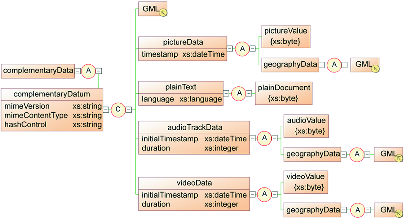
Thus, Fig. 5 details the alternatives for the complementary data related to a given measure. As it is possible to appreciate in Fig. 5, under the complementaryData tag is possible to find a set of the complementaryDatum tag. Each complementary datum must be one of five alternatives: (i) A document organized under the Geography Markup Language (GML)5; (ii) A picture describing the context or some characteristic of the entity under analysis; (iii) A plain text which is possible to be associated with a system log; (iv) An audio track representative of some attribute or context property related to the entity or its context respectively; and (v) A video file which could describe some interesting aspect of the region.
Each complementary datum could be associated with a GML document for describing the specific location. This is useful when the audio, picture or video file should be related to a particular localization. Moreover, the geographic information could be linked in relation to a measure without the necessity to have an associated audio, picture or video file. That is to say, the incorporation of the geographic information does not require the mandatory use of the multimedia files to be included as a complementary datum for a given measure. In this sense, each measure could have complementary data (i.e. it is optional), and in that case, the set could be integrated by one or more complementary datum without a specific limit.
In this way, the CINCAMI/Measurement Interchange Schema allows coordinating the meaning and data organization based on the extended C-INCAMI framework, jointly with the project definition. This fosters the data interoperability between the involved processing systems and the data sources, because the data generation, consuming, and the processing itself are guided by the metadata (i.e. the project definition). For example, the Arduino One receives the project definition by mean of a CINCAMI/PD message, and thus, it knows the range of expected values from the sensor DHT11 (environmental humidity). Then, a value such as 120 could be detected as not valid in the measurement adapter by mean of the direct contact with the data source (DHT11 sensor), just using the metric definition (see Table 2). When this happens, it could be possible to send an alarm to the data processor and discard the anomalous value avoiding overhead from the source.
4.2 The CINCAMIMIS Library
The CINCAMIMIS library is an open source library, freely available on GitHub6 for using in any kind of systems which require the measurement automatization based on the extended C-INCAMI framework. The library was developed in the Java 8 language, using Google gson7 jointly with JAXB libraries.
The library allows generating the measurement streams under the CINCAMI/MIS for being interchanged among the processing systems, the data sources and the processing system, or even the data sources with each other (e.g. in IoT). Thus, the measurement interchange schema fosters the data interoperability independently of the processing systems (be it a data consumer or producer) and the software used for carrying forward the project definition.
Both XML as JSON data formats are supported for making as easy as possible the data interchanging. Complementarily, the GZIP compression can be used on the XML/JSON messages for minimizing the interchanged data and the required time for the communication.
The library implements a translating mechanism which allows transparently migrating among XML, JSON, the object model in any sense. The Object Model is completely based on the extended C-INCAMI framework, a reason why the concepts and terms able to be processed are completely known.
5 An Architectural View for the Measurement Processing
The Processing Architecture based on Measurement Metadata (PAbMM) is a data stream engine encapsulated inside a Storm Topology. It allows carrying forward the data-driven decision making based on the real-time monitoring of one or more measurement and evaluation projects [24].
From the architectural view, it could be analyzed from four functional perspectives: (a) The Definition: It is responsible for the measurement and evaluation project definition. The result of this perspective is a CINCAMI/PD file used as input in the architecture; (b) The Data Collecting and Adapting: The Data Collecting and Adapting: it is responsible to implement from the data collecting on the sensors to the consolidated data receiving for its central processing; (c) The Analysis and Smoothing: It allows carrying forward a series of statistical analysis on the data stream for detecting anomalies, deviations or unexpected behavior in terms of the typical data distribution; and (d) The Decision Making: In case of some situation is detected, it is responsible for making a decision based on the experience and previous knowledge available on the organizational memory. The four perspectives are synthetically described through the BPMN notation in the next section.
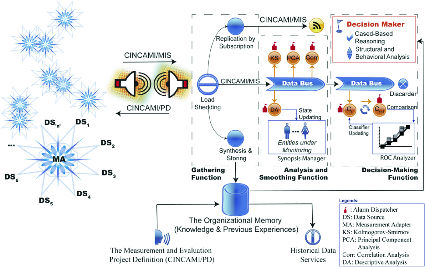
The architectural view for the measurement processing
As it is possible to see in Fig. 6, the Measurement Adapter (MA in Fig. 6) has a morphology like a star. That is to say, each extreme of the star represents a given data source (e.g. a sensor) communicated with the measurement adapter located on the center. Each sensor could be heterogeneous, and for that reason, it is possible that the MA receives the data organized in a different way (a typical aspect in IoT).
Using the project definition file (i.e. the CINCAMI/PD file associated with a given project) in the configuration stage, the MA identifies and knows each related sensor, its associated metric, the quantified attribute or context property, and the entity under analysis.
Synthetically, the MA receives the data organized in a heterogeneous way from each sensor. From there, this is responsible to identify each sensor, verify the obtained measure in terms of the project definition (e.g. for detecting miscalibration), and to make the necessary transformations for sending the measures as a unique CINCAMI/MIS stream.
It is important to remark that each CINCAMI/MIS stream jointly inform the measures and the associated metadata. Thus, the Gathering Function responsible for receiving the data streams guides the processing using the metadata and the associated project definition (e.g. using the CINCAMI/PD file).
The Gathering Function (see Fig. 6) receives the data stream and it applies the load shedding techniques when it is necessary. The load shedding techniques allow a selective discard of the data for minimizing the loose when the arrival rate is upper than the processing rate [25]. Whether the load shedding techniques be applied or not, the resulting stream organized under the CINCAMI/MIS (i.e. the data organization coming from the MA) is automatically replicated to (i) The subscribers: Each one who needs to read the data stream without any kind of modification could be subscribed it (e.g. it could be made using Apache Kafka8); (ii) The Synthesis and Storing Functionality: it represents a kind of filter for the data stream, which acts before to store the content with the aim of synthesizing it. The synthesizes algorithm is optional, and for that reason, a data stream could be fully stored if no one algorithm was indicated. For example, in the monitoring of the environmental temperature related to the “Bajo Giuliani” lagoon, it would be possible to store a synthesis of the environmental temperature every five minutes (e.g. one value) if no change in it happens. In terms of storing, it would be an interesting optimization of its capacity; (iii) The Analysis and Smoothing Function: It is responsible for the real-time statistical analysis of the data stream.
When the data stream is received in the Analysis and Smoothing Function, it canalizes the data through a common data bus. From the common data bus a set of analysis are simultaneously computed: (i) The Kolmogorov-Smirnov through the Anderson-Darling test [26]: it allows analyzing the data distribution in relation to the expected behavior (e.g. detecting normality when it is present); (ii) The Principal Component Analysis: This analysis is useful for detecting the variability source, mainly thinking in aspects that could get out of control the expected behavior for a given attribute; (iii) The Correlation Analysis: It is carried forward for analyzing the dependence and relationships between the involved variables in the entity monitoring (i.e. a metric could be viewed such as a variable), and (iv) The Descriptive Analysis: it allows updating the descriptive measures related to each attribute and context property of each entity. In this way, the last known state is gradually built. Even, from the last known state, an idea of synopsis could be used for answering in an approximate way when the data source related to an entity has been interrupted. As it is possible to see in Fig. 6, some circles have an associated flag but not all. The circles with an associated flag represent that the related operation can launch an alarm when some atypical situation is detected (based on the project definition). For example, when the descriptive analysis is processing the value of the environmental temperature (i.e. a metric’s value, the measure) in the “Bajo Giuliani” lagoon, a temperature upper than 50 °C is atypical for the region, and it could be indicating a fire.
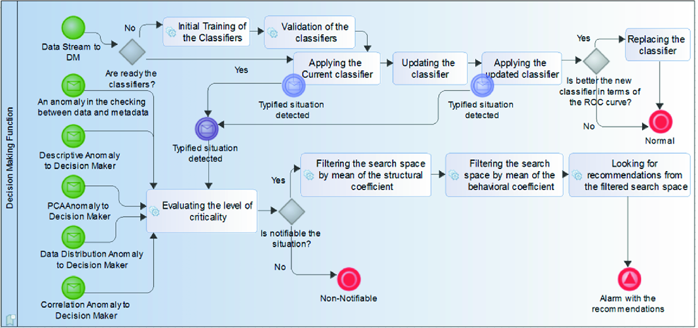
At the same time in which the data are statistically processed, they continue its travel to the decision-making function. In the decision-making function, a current classifier (see Ct in Fig. 6) based on the Hoeffding Tree is applied from the known situations [27]. For example, in the case of the “Bajo Giuliani” lagoon, the known situations could be the fire, flood, etc. In parallel, the original classifier is incrementally updated with the new data, resulting in a new Tree (see Ct+1 in Fig. 6) for who a new classification is obtained. Both classifiers are compared based on the area under the ROC (Receiver Operative Curve) curve [25], and the classifier with the biggest area will be the new “current classifier”. However, and as it is possible to see in Fig. 6, the classifiers could launch an alarm when some critical situation is detected (e.g. a flood). In any case, the alarm receiver is the decision maker component in the decision-making function.
When the decision maker receives an alarm (be it from the statistical analysis or the classifiers), it looks in the near history related to the entity under analysis for similar situations and its associated recommendations. When the situations and recommendations are found, the recommended actions are performed (e.g. notify to the fire station). However, it is highly possible that some entity has not a recent associated story. In such case, a case-based reasoning based on the organizational memory is carry forward supported by the structural and behavioral coefficients. On the one hand, the structural coefficient allows identifying the entities who share the similar structure for the monitoring. On the other hand, the behavioral coefficient allows identifying the entities who experiment a similar. Both coefficients, structural and behavioral, allows filtering the in-memory organizational memory for limiting the search space and improving the performance of the case-based reasoning.
As it is possible to appreciate, the architectural view considers from the project definition, passing through the data collecting (i.e. by mean of the IoT sensors) and adapting (i.e. the measurement adapter) and ending with the real-time decision making and the associated recommendations. The next section introduces the process formalization for the Architectural View related to the measurement processing.
6 The Formalization Related to the Architectural View
The Architectural View of the Measurement Processing is substantiated around five main processes: (i) The configuration and startup: It is responsible for the initialization of the processing architecture, from the loading of each project definition to the start of the data receiving; (ii) The collecting and adapting: It is oriented to warranty the data collecting from the sensors, the needed transformations from the raw data and the delivering to the GF of the data stream; (iii) The Data Gathering: It is responsible for the data gathering coming from the measurement adapters, jointly with the data replications and synthesis when it is required; (iv) Data Analysis and Smoothing: It performs the real-time data analysis based on the M&E project definition, being responsible for the building and keeping of the synopsis in memory; and (v) Decision making: It receives the alarms thrown from the different processes, and it is responsible for determining the necessity of notification based on the priority, informing the actions and the associated recommendations. Following, each process is synthetically explained using the BPMN notation for better understanding.
6.1 The Configuration and Startup Process
Before the processing architecture can process anything, the M&E project definition must be loaded in memory and initialized. As was introduced in Sect. 3, the project definition establishes the information need, the entity under analysis, the attributes used for characterizes the entity, the context properties useful for detailing the context in which the entity is immersed, among other concepts and terms. The loading activity implies read each CINCAMI/PD content from the files or web services, validate it and prepared the data structure and buffer for receiving the data.

The configuration and startup process using BPMN notation
The thread associated with the project definition loader is located in the superior region of Fig. 7, and it starts with the reading of the project definitions. In the beginning, the M&E project definitions are read from the organizational memory related to the PAbMM (see Fig. 6). Each project definition is organized following the CINCAMI/PD schema, which allows using any kind of software for carrying forward the project specification.
Once the definitions were read, the architecture counts them and in case of there not exists definitions, the architecture keeps waiting for new definitions. The waiting time could be specified as an architecture parameter. However, when at least one definition is present, it is updated in memory indicating the entity, the expected attributes, and the associated metrics jointly with the expected values, among other aspects indicated in the definition. If there is not enough memory during the initialization, a fault is thrown, and an abnormal end state is reached.
After the project initializing, the data buffers are created and reserved specifically for the M&E project. Thus, the memory space for the data stream, the synopses and the partial results derived from the statistical analysis are ready for the processing. Thus, a message indicating the “Successful” updating is sent to the project director, and the architecture finally comes back to the waiting state waiting for new definitions (be it new projects or updating).
The thread related to the online updating just implies a task continuously waiting for a message from the project director. When the project director sends a CINCAMI/PD document through a web service to the process by mean of the “Online Updating” message, the architecture migrates the new definition to the project definition loader for starting its loading as was explained before. In this case, and on the one hand, when the successful loading of the new definition is made, the project director receives a message indicating it. On the other hand, and when some memory failure happens, an error message is communicated to the project director too.
The power-off is simple but quite different because it implies the stopping of the data processors, the cleaning and freeing of memory. The manager is the only role able to carry forward the shutdown. Thus, when the manager sends the shutdown signal, the message is received and immediately the data processors are stopped. Next, any transitory results are stored on the disk for finally cleaning all the memory (data structures and buffers). When the cleaning has ended, the architecture sends a message to the manager committing the shutdown.
It is clear that this process is dependent on the project definition, and for that reason, there is not any processing in absence of the project definition. This is a key asset because it allows highlighting the importance of the metadata (i.e. the entity, attributes, metrics, etc.) at the moment in which each data should be processed. Having said that, it is possible to highlight that all of the other processes directly depend on the configuration and startup process.
6.2 The Collecting and Adapting Process

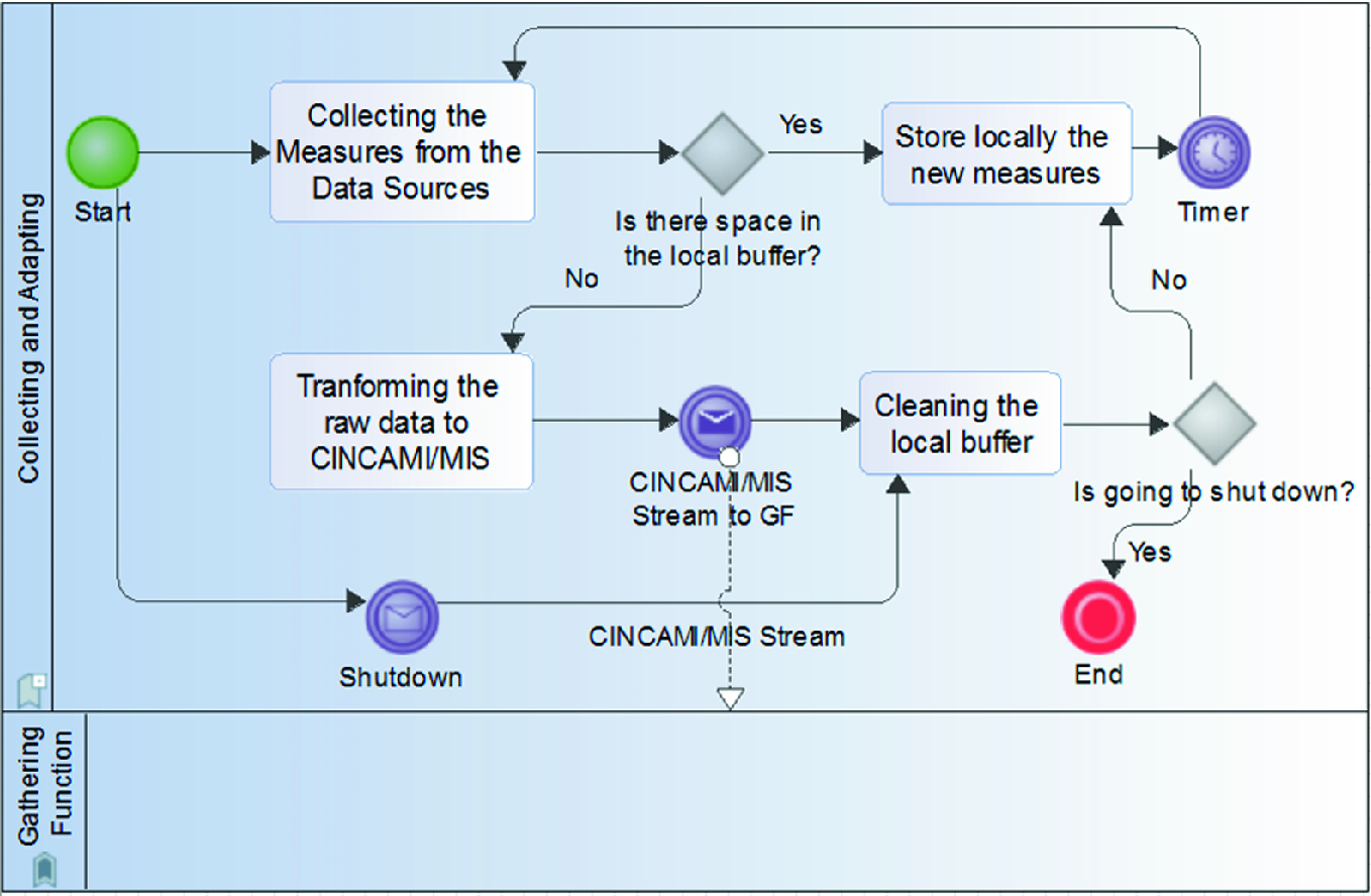
The collecting and adapting process using BPMN notation
As it is shown in Fig. 8, the process could carry forward a new project definition, an updating or even the power-off of the measurement adapter. In this sense, it is important to highlight that the power-off is specifically limited on one measurement adapter and not all the processing architecture. Thus, a set of sensors could be interrupted through the power-off of its associated measurement adapter, while other measurement adapters continue sending data to the gathering function.
The project definition is entered by mean of a CINCAMI/PD definition. The definition could be obtained from: (a) a file, (b) the organizational memory or, (c) by the web services related to the architecture (see Fig. 6). In the case of the CINCAMI/PD definition is locally stored on the measurement adapter, the project loader directly starts with the loading when power-on the device. Thus, a matching between sensor and metrics based on the project definition using the metadata (see Tables 1 and 2) is automatically made. In the case of all the metrics are correctly associated with the sensor, the buffers are initialized, and the data collecting is immediately started.
However, in case of some metric keeps without association, it provokes that the measurement adapter transits to wait for a new M&E project definition. This allows defining a norm such as: “A measurement adapter will initialize an M&E project definition if and only if all the included metrics have an associated sensor in the measurement adapter, else the definition is not appropriated”. In other words, a measurement adapter could have more sensors than metrics, but a metric must have an associated sensor.
In addition, the project director could update the definition sending a new definition to the measurement adapter. The measurement adapter receives the new definition, validate it (e.g. the content and the association between sensors and metrics), starts the new buffers in parallel for instantly replacing the previous definition. Next, the data collecting is continued based on the new definition.
Details on the collecting activity for the collecting and adapting process using BPMN notation
Once the data buffer becomes full, the measurement adapter generates the CINCAMI/MIS stream guided by the project definition. The data stream is sent to the gathering function, after which the buffer is cleaned for continuing the data collection.
This process depends on the “Configuration and Startup” process because the project definition is needed, and the gathering function should be operative for receiving the collected data from the measurement adapters.
6.3 The Data Gathering Process
The Gathering Process is responsible for the data gathering coming from the measurement adapters, jointly with the data replications and synthesis when it is required. Once the processing architecture has been initialized and the measurement adapters too, the gathering function incorporates a passive behavior. That is to say, each measurement adapter sends the measurement stream when it needs, and for each request, the processing architecture will give course to the respective processing.

The data gathering process using BPMN notation
However, when the informed message from the measurement adapter corresponds with an active adapter, the next step is associated with the consistency verification related to the message itself. Thus, the message is effectively read and received, and then, the schema validation is carried forward. In the case of the stream does not satisfy the CINCAMI/MIS schema, the process instantiation is derived to the end state indicated as “Inconsistent Stream”.
Thus, all the streams which satisfying the measurement interchange schema (i.e. CINCAMI/MIS) are derived for the application of the load shedding techniques. The load shedding techniques allow a selective discarding based on the content stream and the M&E project definition. This kind of optional techniques is automatically activated when the arriving rate is upper to the processing rate. Because the measurement interchange schema is completely based on the M&E project definition, it is possible to retain in a selective way the priority measures.
Once the measurement stream has passed through the load shedding techniques, the resulting measures are replicated. The replication happens to four different destinations: (a) The subscribers: It requires a previous registration for continuously receiving the measurement stream without any modification; (b) The Analysis and Smoothing Function: a copy of the current measurement stream is sent for the real-time statistical analysis; (c) The Decision-Making Function: a copy of the current measurement stream is derived for analyzing whether corresponds with some typical situation or not (e.g. fire, flood, etc.); and (d) Historical Data: Basically the measurement is directly stored in the organizational memory for future use. However, when the synthesis data option is enabled, the measurement stream is processed through a determined synthesis algorithm which internally determines what kind of data must be retained and stored. For example, it is possible to continuously receive the temperature data from the “Bajo Giuliani” shore, but maybe, it could be interesting just keep the temperature’s changes in persistence way.
Thus, when the measurement stream has been derived by mean of the four channels (i.e. the subscribers, analysis and smoothing function, decision-making function and the organizational memory), the process comes to its end.
6.4 The Analysis and Smoothing Process
The Analysis and Smoothing Process performs the real-time data analysis based on the M&E project definition, being responsible for the building and keeping of the synopsis in memory.

The analysis and smoothing process using BPMN notation
The Descriptive Analysis allows checking each measure in terms of the project definition, and at the same time, carry forward the updating of the descriptive measures (i.e. mean, variance, etc.) for each metric related to a given entity under analysis. In this sense, when the descriptive analysis obtains a value inconsistent with the project definition (e.g. an environmental temperature with a value of 200), an alarm is sent to the Decision Maker. Whether the alarm is thrown or not, the computed descriptive measures for each metric allows updating the synopsis related to the entity under monitoring. Thus, by mean of the synopses, the processing architecture could partially answer the state of an entity in front of a given query, even when the associated measurement adapter has been interrupted.
The Principal Component Analysis is carried forward for evaluating the contribution to the system variability of each metric in the context of the M&E project. When some metric (i.e. or random variable in this context) is identified as big variance contributor, an alarm is thrown to the decision maker for analyzing it. Whether the alarm is thrown or not, the PCA analysis allows updating the synopsis related to each associated entity under monitoring.
The Data Distribution Analysis carries forward the Anderson-Darling test for analyzing the data distribution in terms of the previous data distribution for the same metric. When some variation is detected, an alarm is thrown to the decision maker. Continuously the data distribution information is updated in the synopsis for enabling the future comparison in terms of the new data arriving.
The Analysis of the Outliers is continuously performed for each metric and entity under analysis. When some outlier is detected, an alarm is thrown to the decision maker. The decision maker will determine the importance and priority of each alarm. The outlier information is continuously updated in the synopsis for comparing the behavior in relation to the data distribution.
The Correlation Analysis allows analyzing the relationships between the metrics, be they attributes, or context properties related to a given entity under analysis. Thus, it is important to verify the independence assumptions among the variables (i.e. the metrics), but also for possibly detecting new relationships unknown before.
Finally, all the information coming from each analysis is updated in the last known state by the entity, which allows carrying forward the online computing of the scoring for the recommendations. That is to say, with each new data coming through the measurement stream for a given entity, the recommendations are continuously reordered in terms of the pertinence in relation to the new data. Thus, when some alarm is thrown for a given entity, the scoring corresponds with the last data situation for the associated entity. This avoids an additional computation for the decision making when it needs to incorporate recommendations jointly to the actions for a given alarm.
6.5 The Decision-Making Process
The Decision-Making Process receives the data and alarms from the different processes (i.e. The Gathering Function and Statistical and Smoothing). It is responsible for determining the necessity of notification based on the priority, informing the actions and the associated recommendations.
The decision-making process using BPMN notation
Once the classifiers are trained, each new data is classified by the current classifier. Next, the classifier is updated with the new data, and the data is reclassified using the updated classifier. Both classifiers are compared by mean of a ROC curve. When the updated classifier contains an area under the curve upper than the current classifier, the updated classifier becomes in the new current classifier, replacing it. It is important to highlight that in case of the current or updated classifier give a classification related to a typified situation which is considered critical (e.g. fire, flood, etc.), the process is directly derived for evaluating the level of criticality.
The rest of the start points of this process correspond with alarms thrown from the statistical and smoothing function. All the start points related to a message implies that the anomaly or alarm was detected, and in this process, the criticality analysis should be made.
The level of the criticality is taken from the decision criteria contained in the indicators jointly with the organizational memory, who contains the previous experience and knowledge. Thus, and on the one hand, when the situation is an alarm in where the notification is not required, it is discarded. On the other hand, when the alarm requires notification, the search spacing of the organizational memory (a Big Data Repository) is filtered looking for the associated recommendations, and finally, the external alarm is sent with the actions and associated recommendations (e.g. the steps to follow in a given situation).
Because the organizational memory is a big data repository, the strategy is to keep in memory the most used region. For that reason, the scoring is permanently updated on each new data. In addition, the structural coefficient allows looking for entities which share attributes for its quantification. However, a most strict limitation could be carried forward using the entities with a similar structure, but also with similar behavior for each monitored attribute [28]. In this sense, when there are not recommendations for a given entity, it is possible to find recommendations coming from similar entities for avoiding send an alarm without recommendations. For example, the “Bajo Giuliani” lagoon is a new entity under analysis and there is not associated history. However, in case of fire, the previous experience related to other lagoons, could be used for driving the steps in an emergency.
7 An Application Case Using the Arduino Technology
In this application case, the processing architecture based on measurement metadata is applied to the real-time lagoon monitoring. In this case, the application is associated with the “Bajo Giuliani” lagoon. What is special with the “Bajo Giuliani” Lagoon? It is a natural reservoir of water, located 10 km at the south of the Santa Rosa city (the capital of the province of La Pampa, Argentina), in South America. The lagoon receives the water from the rain and the waterways who bring the derived water from the Santa Rosa city.

The “Bajo Giuliani” lagoon. A descriptive map for the region. The satellite image was obtained through Maps 2.0 (Apple Inc.) with data from TomTom and others
On the south coast of the lagoon, there is a neighborhood named “La Cuesta del Sur”. In this neighborhood, there are one hundred seventy houses and originally, they were used such as weekend houses. Nowadays, there are one hundred families living in the neighborhood, which incorporate a constant traffic by the internal streets and the connection with the routes.
In March of 2017, the volume of fallen water by the rains was excessive for the region related to the Santa Rosa city. Just in three weeks, the volume of water was equivalent to one full year [29]. It provoked that the city keeps partially under the water, generating different kinds of health risks without to enumerate the economic damages. For this reason and in front of this kind of emergency, the water from the city was immediately derived through the waterways to the “Bajo Giuliani” lagoon.
Thus, the volume of derived water through the waterways was constant, and it provoked the incrementing of the level of water related to the lagoon. The concerns started when the water advanced on the land located on the south coast, of the neighborhood, flooding it.
This situation gave origin to this project and the associated application. The indicated points on the south coast of the lagoon in Fig. 13, indicate the initial points established for the installation of the monitoring stations.
Before introducing the monitoring stations, it is important to remark the initial definition of the measurement and evaluation project associated with the lagoon and introduced in Sect. 3. The project’s information need could be defined as “Monitor the level of water of the ‘Bajo Giuliani’ lagoon for avoiding flood on the south shore related to the neighborhood”. The entity category is defined such as “lagoon located in the province of La Pampa. The entity under analysis or monitoring is limited to the “Bajo Giuliani” lagoon. The attributes chosen for characterizing the lagoon are (i) The water temperature, (ii) The ground moisture, and (iii) The water level. The context of the lagoon is described by the following context properties: the environmental temperature and humidity. In this particular case, the incorporation of a camera as a complementary datum is an added-value for describing the region in case of necessity (see Sect. 4.1, Fig. 5).
The Processing Architecture based on Measurement Metadata is located in terms of physical processing in the region indicated as “Base Station” in Fig. 13. The firsts monitoring stations were installed from the south-west coast to the south-east region of the lagoon because the neighborhood is located in a hill, being the south-west coast the lower region. The slope of the hill goes growing-up from the south-west to the south-east coast, being the riskiest region the south-west coast of the lagoon.
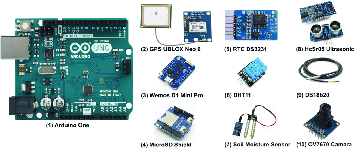
Set of components based on the Arduino one used for building the monitoring station
Complementarily, the monitoring station incorporates the complementary data through the GPS UBLOX Neo 6 (see Fig. 14, the component with ID 2) for obtaining the georeferentiation associated with the measures, and the OV7670 camera for taking pictures when it is necessary (see Fig. 14, the component with ID 10). This is an interesting aspect, because the measurement interchange is not only about the estimated or deterministic values related to the metrics, but also the pictures and/or geographic information which allows showing the capacity to interact with embedded multimedia data.
Finally, a real-time clock is incorporated for timestamping the DateTime in each measurement (see Fig. 14, the component with ID 5), jointly with a microSD shield useful for implementing the local buffer in the measurement adapter (see Fig. 14, the component with ID 4).
Thus, this kind of monitoring stations is accessible to everyone who needs to reproduce this kind of experience, even in other sector or industry, such as the agricultural for soil monitoring.
The application allows a real-time monitoring of the level of water related to the lagoon, evaluating at the same time the effect of the summer or spring season and its incidence in the water evaporation. The neighbors and the local governments could access to the real-time measures for knowing the current state of the lagoon, they could receive the flood alarms before the situation happens, and the local governments could regulate the volume of derived water through the waterways when this is possible.
8 Related Works
The idea related to collect data from different kind of data sources is not new, just that now the technology and the computing power made possible new perspectives, applications and, data processing alternatives. Ferdoush and Li [30] have proposed an overall system architecture based on the Raspberry Pi9 and Arduino10 Technology. The work presented a wireless sensor network with the aim of environmental monitoring, which is based on open source hardware platforms for keeping the cost low and facilitating the maintaining of the devices. Vujović and Maksimović [31] developed an architecture for home automation using the RaspberryPi as a sensor web node. A comparison among with the similar hardware platforms in relation to the application case was presented. Both proposals define the data gathering and its associated processing based on open source hardware, leaving the measurement definition as an open aspect, which could have some inconvenient in terms of the result comparisons or when the measurement process should be extended (i.e. the descendent compatibility). In this sense, PAbMM formalizes each operational process, describing through the measurement and evaluation framework, each involved concept with an entity under analysis.
Stephen et al. [32] described STYX, a stream processing with trustworthy cloud-based execution. This proposal makes focus on the confidentiality specifically related to the interchanged data between each device and the data processor in a wireless sensor network. A proposal in an analogous line is introduced by Ghayyur and others by mean of the IoT Detective game [33]. This aspect takes a particular importance when a solution wishes to be generalized satisfying the different kinds of regulations related to the data interchange along the world. For this reason, the measurement interchange schema (see Sect. 4) embeds metadata based on the project definition, which allows knowing the data origin, it keeps the data traceability, it knows the measurement adapter (the intermediary between the data source and the data processor), it incorporates the integrity control inside each cincamimis message with the possibility of protecting its confidentiality.
Andrade et al. [34] present a study in which analyze the behavior of heterogeneous devices (e.g. IoT devices) in a car (i.e. connected cars) based on radio connectivity. The underlying idea is to measure the consuming pattern (e.g. mobility) of the resources on a GSM production network with around one million of the radio connections from the cars. It is an interesting analysis for taking dimension of the data traffic in a tangible domain related to IoT on road. In this sense, PAbMM incorporates the mechanism for online monitoring each data stream in terms of the active projects jointly with the available resources, which takes a particular interest when the decision must be made in real-time (see Sect. 5).
Carvalho et al. [35] introduce the processing of distributed data streams based on an architecture oriented to IoT smart grids monitoring. The architecture relationships the IoT with the heterogeneous data sources contained in the sensor networks, making a focus on the smart grid data profiles. In this approach, Apache Kafka11 is used on the message layer, while the processing layer is based on Spark Streaming.12 It is a similar view in relation to PAbMM, but the main difference is associated with the way in which the monitoring project is defined, and the data interchange. That is to say, PAbMM uses a measurement and evaluation framework as the underlying supporting for the project definition, giving existence to the CINCAMI/Project Definition. Even, the measurement interchange schema (i.e. CINCAMI/MIS) is the way in which heterogeneous data sources and the data processor carry forward a common understanding in relation to the data meanings, the associated project, and its entity under monitoring (e.g. 38.3 is a temperature coming from a sensor monitoring the child’s corporal temperature in Fig. 2).
The data collecting jointly with the data processing for supporting real-time decisions currently has different kinds of applications, some of them are: (i) the role of the fog computing, IoT and cloud computing in the healthcare 4.0 for providing uninterrupted context-aware services [36]; (ii) The role of the IoT and smart grids in the context of the smart cities [37]; (iii) Aspects related to the security alert systems for smart home [38]; (iv) The vehicle air pollution monitoring based on IoT devices [39]; (v) The role of the ontology for the platform scalability in the complex IoT contexts [40], among others. In addition, the multimedia big data implies the proliferation of the multimedia data in the big data repositories (e.g. audio, video, etc.), and this aspect was introduced with the complementary data in the measurement interchange schema (see Sect. 4). In this sense, taxonomies and a model process are described in [38], addressing different kinds of challenges in the area, such as the reliability, heterogeneity, etc. In this line, PAbMM has an underlying ontology based on the measurement and evaluation framework named C-INCAMI, which is used for the project definition (i.e. CINCAMI/PD) and the measurement interchange schema (i.e. CINCAMI/MIS). Thus, each actor in the architecture knows the responsible sensor for an attribute, the associated meaning, the way in which the data should be processed, and the normal behavior patterns defined by the experts in the project definition (coming from the organizational memory).
9 Conclusions and Future Works
Nowadays the different kinds of the data sources and its evolution, carry us to a heterogeneous environment in which each time the components trend to keep a continuous interaction as a form to self-organizing for satisfying a given objective. In this environment, the heterogeneity is the norm which rules the different applications, be it through the sensors or even the kind of the data that need to be processed (i.e. from the raw data to the information geographic in its different forms). Moreover, the data sources (i.e. sensors) are permanently generating data for its processing and consuming. Thus, and when the data should be stored (synthesized or not) the volume and the associated rate of the data is increased in a significative way falling in the Big Data environment. Nowell, the online data processing is a very different context than the Big Data environment, because when in the first the real-time data processing is a priority, in the second the batch data processing is the rule. This is important to highlight because the data processing strategies are very different like the needed resources for carrying forward the processing in its different forms. In this sense, the chapter introduced an integrated perspective for the data processing in the heterogeneous contexts, incorporating the process description through BPMN.
The measurement process is a key asset when the monitoring must be carried forward on a given target. In this sense, the determination about the concept or object to be monitored jointly with the way in which the measurement is carried forward constitutes the base for the data-driven decision making. That is to say, the decision maker must support each decision based on the information and not the mere intuition.
Thus, before any kind of the data processing for the data coming from the sensors, it is necessary to warranty the processability and the understandability related to the data to be processed in terms of the measurement process. For that reason, this chapter introduced the idea of the measurement and evaluation framework (e.g. C-INCAMI), like the way in which the measurement process could warranty the comparability of its results, the repeatability, and extensibility of the process itself. For example, the C-INCAMI framework allows using the terms, concepts and its relationships for defining the information need of the project, the entity to be monitored, the descriptive attributes for the entity, the descriptive context properties for the environment in which the entity is located, the associated metrics, among other essential aspects for knowing the way in which each aspect related to an entity under monitoring is quantified.
In this way, the CINCAMI/Project Definition (PD) schema was presented as the way in which the M&E project definitions based on the C-INCAMI framework could be interchanged among different systems, independently of the creator software. It is interesting because fosters the interoperability in terms of the project definitions, avoiding the dependence of a particular or proprietary framework. The C-INCAMI/PD library which allows the supporting, interchanging and interpretation of each project definition under this schema are, it is open source and freely available on the GitHub repository.
In a heterogeneous environment and when it is possible to agree on the way in which an entity will be monitored, then it is possible to understand the role of each metric (or variable) in relation to the entity under monitoring jointly with its expected incidence. Thus, starting from a definition based on the CINCAMI/PD schema, the chapter introduced the role of the measurement adapter in terms of its relationship with the sensors who show a passive behavior. The measurement adapter allows carrying forward the data collecting, but also the translating of the heterogeneous data from its proprietary data format to the measurement interchange schema (i.e. CINCAMI/MIS). The measurement interchange schema allows homogenizing the data interchanging based on the project definition and the underlying concepts and terms coming from the measurement and evaluation framework. This is a key asset because the data collecting and processing are guided by the metadata and the metadata are directly associated with the way in which an attribute or context property should be quantified and interpreted. The measurement interchange schema has an associated library freely available on the GitHub repository useful for fostering the use and interchange of the measures based on the project definition. For this reason, Both the measurement adapter and the processing architecture are able to carry forward the data collecting and processing respectively because they share a common definition and communication language. That is to say, in case of the use of the deterministic measures or the incorporation of complementary data (e.g. a picture, a video, etc.), the measurement adapter knows the way in which the association sensor-metric should be made following the project definition, and in addition, it knows the way in which the same information should be informed through a CINCAMI/MIS stream. In an analogous way, the processing architecture knows the way in which each CINCAMI/MIS should be read, and by the use of the project definition, the architecture knows the role of each attribute or context property in relation to the project’s aim jointly with the role of the eventually informed complementary data.
The processing architecture incorporates the real-time data processing on the measurement streams, incorporating a detective behavior through the statistical analysis and the analysis of the project definition, jointly with a predictive behavior based in the use of the incremental classifiers. The architecture contemplates the possibility of replication of the measurement streams jointly with the storing of the data, be it in a direct way or by mean of a synthesis algorithm. In any case, the role of the processing architecture when some typified situation or alarm happen, is looking for recommendations for attaching to the notification to send. For this reason, an organizational memory is used as a guide for capitalizing the previous experience and the knowledge from the experts, but also for storing the project definitions, the historical data and the training data set for the initial training of the classifiers.
A real application of the processing architecture was synthesized for the lagoon monitoring and its incidence in the “La Cuesta del Sur” neighborhood (Santa Rosa, La Pampa, Argentina). This kind of applications and the positive social impact for the governments, people and the private organizations allows projecting many kinds of the business plan and social applications, from the farm monitoring, flood monitoring, fire monitoring, among a lot of applications, in which the real-time monitoring could positively increment the benefits and the profits with a minimal cost. That is to say, the investment related to each monitoring station is minimum (e.g. around 50 dollars depending the precision, accuracy, and kind of sensors to be used), and the involved software is open source reason which there is no additional cost.
The semantic similarity related to two or more entity under analysis is an active researching line. That is to say, the entities are characterized by the attributes in terms of the C-INCAMI framework. Each metric is directly associated with an attribute (or context property). The current structural coefficient is used for the in-memory filtering of the organizational memory looking for the entities that share as many attributes as possible. Thus, in case of absence of recommendations for an entity, it is possible to reuse the previous knowledge from other similar entity. However, the structural coefficient is based on the attribute comparison by the name, but not based on its definition (i.e. the meaning). Thus, the active line refers to obtain a semantic coefficient able to be applied to the Spanish language, for knowing when two attributes for the same entity correspond to the same concept based on a narrative definition (i.e. the explanation of the meaning of each attribute given in the project definition), independently the given name to each attribute.