4
Data Preparation
4.1 Necessity of Data Preparation
Having obtained useful data, it now needs to be prepared for analysis. It is not unusual to have the data stored at quite a detailed level in a data warehouse. But to get relevant, reliable and repeatable results out of the analyses, transformation and aggregation of the data is necessary. The type of aggregation has a major impact on the final result. It is unlikely that data mining algorithms will find hidden patterns without prior data preparation. Even if the user doing the data mining is not able to do the transformations and aggregations, it is important for the user to define the necessary steps and make sure someone else does them, for example, colleagues in the IT department. Most of the time, it is also useful to apply domain knowledge in the way the data preparation is done, for example, taking advantage of knowledge of the usual range and type of data items.
4.2 From Small and Long to Short and Wide
In most data warehouses, you are faced with data structures that have a central part with multiple associated areas attached in a structure somewhat similar to a snowflake. Let us say that in the centre is quite a big fact-based table where each row represents a detailed piece of information, for example, regarding customer behaviour, or payment attributes, or production details, or advertising and sales campaigns. This centre fact-based table is connected by key variables to other fact-based tables, for example, key variable orders connected to payments, and each of the fact-based tables is surrounded by multi-dimensional tables that give additional information to the keys used in the fact-based table.
Consider the simple example for a manufacturer in Figure 4.1 .
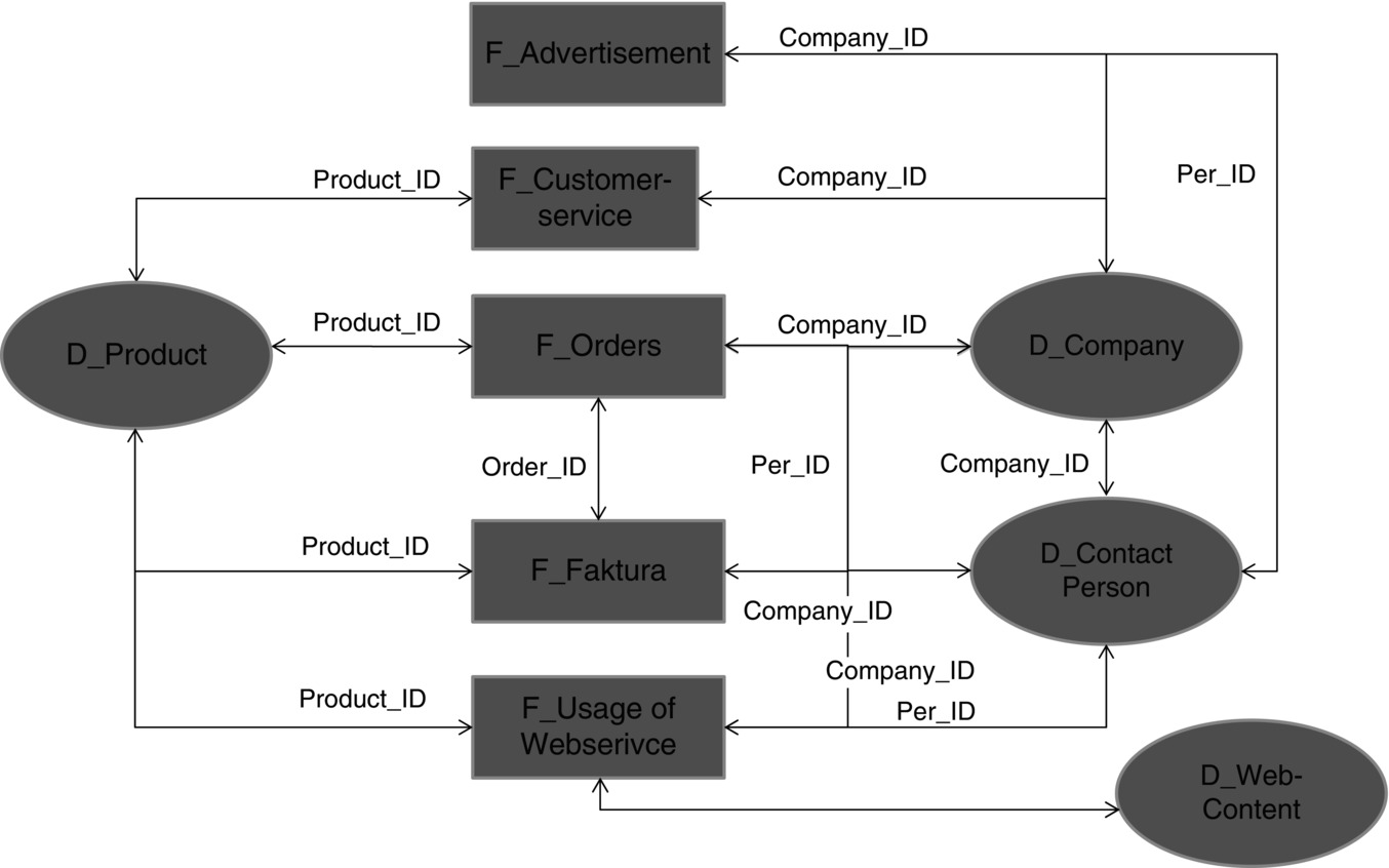
Figure 4.1 Typical connections between fact tables.
If you have a closer look at the ‘orders’ in the fact table in Figure 4.2 , you will notice that the same customer is represented in more than one record. To describe the customer’s behaviour and to make him or her suitable for most of the analytical methods, you need to sum the records up somehow. The easiest way might be to sum everything; but information collected yesterday does not always have the same value as that collected more than two years ago. The business may have changed dramatically over the years. Therefore, a weighted sum may be more suitable with some of the data having more importance than other data.

Figure 4.2 An example of an order fact table.
In Figure 4.2 , the first column is the row number, the second column is Firmen_Num for company ID and the next column is Kunden_Num for customer ID, followed by Auftrags_Num for order, invoice or receipt number; Bestell_Datum for order date; Order_sta for order status; and then two variables to identify which advertisement generated the order. The final two columns are Betrag_Auftrag for order value and Zahl_Art for how it is paid.
In this excerpt of an order fact table, notice that, for example, rows 84040–84047 have the same customer ID and there are seven different order IDs. The oldest order dates back to the year 2011 and the youngest to the year 2013. This example shows that a single customer can appear in several rows of the order fact table, each row corresponding to a different value for one of the other variables: product, order and date.
If the subject of our analysis is the customer, we should plan to end up with just one row for the customer, for example, Kunden_num 374172. If the subject of our analysis is the company, we should plan to end up with just one row for the company.
If we carry out a simple screening of all the rows, we might come up with the following in Figure 4.3 with either company as subject or customer as subject.

Figure 4.3 Person as subject – easy.
This is a very easy way to summarise the different records for one subject, but it does not use all the information included in the original data. Regarding reading and simplification, we can change the format of description, and we are just rearranging what is already there. What else can be found in the information at the customer level? Consider defining a particular day, 15 January 2014, and summarising the information as shown in Figure 4.4 .

Figure 4.4 Person as subject – more information.
Sometimes, especially if you are faced with thousands of different products, it makes more sense to choose product groups or colours or some other material information to define the variables. Note that in the end, the data mart should contain information from all relevant fact tables like in the manufacturer example which included advertisement, online information and customer service. This ensures that revenue information, for example, is available in the data mart as well as the click count of online activity as well as numbers of marketing activities.
This example should give an impression and inspiration. There is no overall master plan for carrying out data mining on the available data marts, but it may help you to decide to create new variables if you try to see and cumulate the information under different viewpoints, even if you know that in a statistical sense, it is quite likely that some of the variables are highly correlated. Depending on the domain, you can create hundreds of new variables from a slim fact table (i.e. a table with only a few columns) or a set of connected fact tables to describe each case or subject (mostly cases are customers).
The only statistical reason that might limit your number of variables is the fact that for most of the analytical methods, the number of records or cases in the analytical dataset should be bigger than the number of relevant variables. If it seems that you will be faced with the problem of too many variables and not enough data, follow a two-step strategy:
- Create all variables that come to your mind or are common domain knowledge.
- Use feature reduction methods that help you to find the most relevant variables for your actual problem.
The relevant variable set may vary from analyses to analyses, but note that it is important to recheck that similar problems should have similar variable sets. In case you are faced with the situation that you know from your business (domain) knowledge that two problems are highly correlated but the outcome of your feature reduction is totally different, you must dig deeper to solve the problem or be totally sure of the results. Otherwise, you run the risk of creating unstable models, or you may lose a brand new business rule that might have arisen as part of the outcome.
4.3 Transformation of Variables
Recall that in the example earlier, the data in the data mart may have different scales and sometimes even different measurement levels. For most of the analysis, it is an advantage if the variables have comparable scales and similar measurement levels. Not all measurement levels are suitable for every kind of method without additional transformation. Figure 4.5 gives an overview of the interaction between measurement level and data mining method.
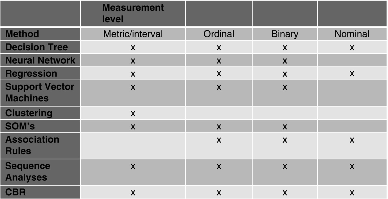
Figure 4.5 Interaction between measurement level and data mining method.
Note that the descriptions of most of the common data mining software tools give the impression that every method can be used with any measurement level. This is only half of the truth. What it really means is that the tool includes automatic methods to transform the data to a suitable level; a well-known example is the transformation from nominal data to several new binary variables, also known as indicator variables. For example, if the original variable consists of colours like red, blue and green, it will be transformed to three variables – one for red, with a value of 1 if the original variable is red and value of 0 if not; one for blue; and one for green – each following the same pattern. In most cases, the automatic transformation is fine and suits the need, but there are cases where it might not be the best solution. For example, it may be that an ordinal scale is really more appropriate such as white = 1, grey = 2 and black = 3. In this case, the required transformation has to be done manually. This kind of transformation and the associated algorithm must be defined using your domain knowledge. For example, the first model constructed using the automatic transformation might miss out rules that you might have expected based on your business knowledge. If these missed rules are related in some way to the critical variable, you would be well advised to do the relevant transformation by hand and redesign the model and then compare the results.
Depending on the chosen or planned data mining method, different scales might have a big influence on model stability and results. Consider these challenges:
- Missing data
- Outliers
- Data with totally different scales
- Data with totally different distributions
4.4 Missing Data and Imputation Strategies
Based on the fact that data for the majority of data mining projects is observational data collected from existing processes as opposed to well-designed experiments, missing data is a common problem. To fix it, we have to distinguish between ‘real missing data’ and ‘not stored information’. Typical examples for real missing data are missed birthday or age information in marketing problems or temperature or moisture measurements in manufacturing datasets. Real missing data occurs in datasets generated from situations where the information itself for sure exists in real life, but for unknown reasons, the information is not stored in the dataset. For example, every customer actually does have an individual age, and he or she is actually born on a particular date even if that data is missing. The data may be missing because of an explicit wish of the customer not to share the information or because some process or other for obtaining the information has not worked correctly. Missing information on temperature or moisture or such like is very dependent on process errors or technical errors.
If real missing data is detected, then it can be replaced by estimation using imputation strategies. The estimation method differs depending on the business context and on other existing information. Estimation can be by replacement using the mean or median (calculated over all data or just a relevant subset) or may be by a more complex method such as using a regression equation or a time series analysis. Cases with missing variables are only rarely excluded.
An alternative way to replace real missing values is to use third-party knowledge. For example, a look-up table can be used to deduce gender from first names, like Mary = female and John = male. If such a table is not available, then you have to construct one yourself based on the full dataset that you have. Make sure that you use the same coding, for example, if your full dataset uses 1 = male, then you should create a look-up table with 1 = male as well. To combine the dataset containing missing values with the look-up table, you should merge both tables using the first names as key. You can also create a look-up table from the salutation (i.e. Mr(Herr) or Ms(Frau)) (see Figure 4.6).
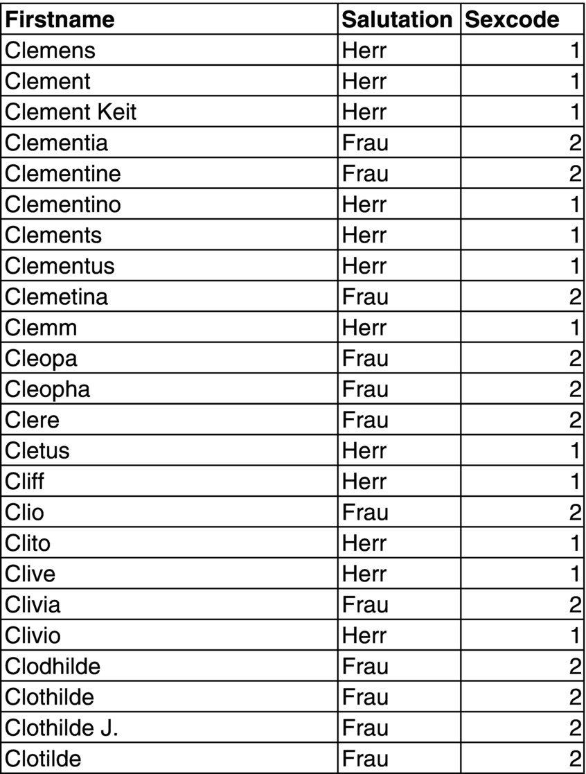
Figure 4.6 Example of a look-up table.
Missing data that represents ‘not stored information’ is very different to the cases of real missing data; they have to be replaced by zero or another value that represents the business knowledge behind it. These cases happen because most company databases just store things that happened and not things that have not happened. An example is that customers ‘who buy’ create footprints in the database; that fact is stored in several tables in which you will find the purchase date, amount, value, products, the way they are ordered, paid, delivered and so on. For those customers ‘who did not buy’, you will find nothing in the company databases at that time. But for some analyses, it is important to represent the ‘not buying’ fact as well in the dataset that should be used for data mining, especially if ‘not doing something’ is done by the majority of people.
Instead of representing the ‘not happened case’ by zero, you can also count the number of days since the last time something happened. Note that this kind of missing data has to be replaced with a value indicating the business meaning, but in addition it should fit with the preferred analytical method. For example, every ‘no buy’ can be represented by zero if the variable itself contains values (money) or amount (pieces). If it contains ‘days since’, then you cannot represent the missing data with zero because that would wrongly lead you to the interpretation that something happened just recently. Here, it may be better to use the number of days since the last known activity (e.g. subscribe for an email newsletter) for estimation or other similar substitutes that correspond with your business rules.
Consider the following example:
Customers: A and B bought in the last six months; C and D did not buy in the last six months.
Today’s date: 10.12.2011
| Customer A: entry 06.06.2000 | Purchases: 04.12.2011 | Product 1234 | 4 999 € |
| Customer B: entry 28.04.2001 | Purchases: 07.12.2011 | Product 1234 | 4 999 € |
| Customer B: entry 28.04.2001 | Purchases: 15.11.2011 | Product 5678 | 14 999 € |
| Customer C: entry 23.01.2007 | Purchases: 23.01.2007 | Product 1234 | 3 999 € |
| Customer A: entry 06.06.2000 | Purchases: 06.06.2000 | Product 458 | 6 999 € |
| Customer D: entry 06.06.2000 | No purchases at all |
Figure 4.7 shows part of a data mart with missing values.
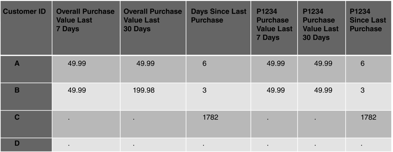
Figure 4.7 Part of a data mart with missing values.
Figure 4.8 shows part of a data mart with replacement for missing values.
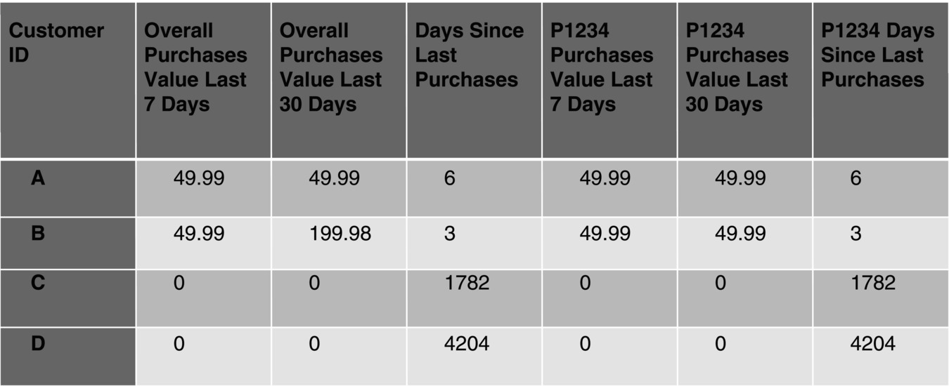
Figure 4.8 Part of a data mart with replacement for missing values.
Note that if a customer pays by cash, there is no automatic record of their details unless they are willing to divulge them or they can be persuaded to use a loyalty card.
4.5 Outliers
Outliers are unusual values that show up as very different to other values in the dataset. Outliers can arise by process errors or through very rare customer behaviour or other unusual occurrences. If it is a process error, you can handle the outlier in a manner comparable to a ‘real missing’ value, or if you have enough cases, you can reject the case that includes the outlier. If you are sure that it is not a process error, then it is quite common to use techniques such as standardisation or binning or the quantile method to mitigate the effect of the outlier. These methods are described in the next sections. Otherwise, it may be sensible to compare the results of analysis with and without the outliers and if there are marked differences to report on both sets of results.
4.6 Dealing with the Vagaries of Data
4.6.1 Distributions
For most of the data mining methods, there are no constraints or only minor constraints about the distribution of the variables. Regression techniques require that target data follows the Normal distribution after allowing for the explanatory variables in the regression. Principal components analysis and factor analysis also require the variables to be Normal.
4.6.2 Tests for Normality
A reasonable test for Normality is to look at a histogram of the data. If the histogram is approximately bell shaped and symmetrical, then the data can be assumed to be approximately Normal. More precise tests can be used, for example, the Kolmogorov–Smirnov test (see statistical texts in Bibliography). However, when there are large quantities of data, any deviation from Normality will be flagged up as statistically significant. Hence, a visual appraisal is usually satisfactory. Tests for Normality are important as they show up features in the data. A common reason for lack of Normality is that there are really two or more sub-groups within the data. It is important to recognise these, for example, customers from one location may have totally different shopping habits from those from another location. Separate analyses may be appropriate for these sub-groups, or the test for Normality must be carried out after fitting an explanatory variable included to represent location.
Many data items are approximately Normally distributed when they are representative of a distinct subset of the dataset. However, some measures are intrinsically non-Normal. For example, the lifetime of customers is unlikely to be Normal as no one can have a lifetime less than zero, yet some loyal customers can stay with the company for many years; therefore, the distribution will be asymmetrical and can only extend to large values on the positive side. In this case, the histogram will be skewed to the right. Normalisation and ranking or other transformations like a Box–Cox power transformation (see succeeding text) can help to make the data approximately Normal. For positively skewed data, a log transformation is effective for making the data more symmetrical. For left skewed, other transformations have to be tried.
4.6.3 Data with Totally Different Scales
Data from real processes sometimes have totally different scales, for example, dates have a different scale to the number of items sold, to the money that has been paid and to simple binary data like payment with credit card or not. In this case, it is necessary to think about methods that equalise the scales. Again, you can solve this problem with standardisation/normalisation, ranking or binning. These issues are dealt with in the succeeding text.
4.7 Adjusting the Data Distributions
4.7.1 Standardisation and Normalisation
Standardisation usually refers to the process of scaling data so that it has a zero mean and unit standard deviation. This may be carried out to ensure that two or more sets of data have the same scale. The usual reason for carrying out standardisation is to be able to compare the variables.
Standardisation is usually intended to make data Normal, in which case it can be considered to be normalisation. Normalisation is carried out when you need a Normally distributed variable because you want to use an estimation method that requires Normality or at least variables with comparable scales. Note that if you transform using a standard normalisation, you will end up with a variable having a mean equal to 0 and a standard deviation equal to 1. Normalisation is only relevant for continuous data. It is a very common procedure and exists as a function in nearly all data mining or statistical tool sets.
Standardisation and normalisation may make the interpretation of the resulting models and the transformed variables more difficult especially for non-statisticians. If you use normalisation, also available in the common statistical and data mining tools, the transformation will deliver a meaningful and comparable mean on one hand and variable scale in a specific range on the other.
4.7.2 Ranking
Ranking is a possible way to transform the distribution of a variable and is also a good opportunity to deal with business-related outliers. Ranking is very easy to do; some data mining tools provide a procedure for it. Otherwise, you can do it yourself by sorting the variable by size and giving a rank order number for each row. Whether rank one is the highest or the lowest value depends on the domain context. If the new variable should follow the Normal distribution, an additional simple transformation is required.
4.7.3 Box–Cox Transformation
Alternatively, a Box–Cox transformation is done which results in the transformed values being a power of the original. Note that zero remains zero. If the data is unstable so that there are lots of business-related changes, then the Box–Cox method can be too sensitive as it may change with each change in the data; in other words, it is like an over-fitting problem, and it gives the impression of being more exact than is justified. The Box–Cox transformation lacks robustness in our context. However, it can be a useful method if your data is stable.
4.8 Binning
To stabilise and improve the data mining models, it is preferable to classify continuous variables, such as turnover, amount or purchasing days into different levels. Using such a classification, it is possible to stress more strongly differences between levels that are important from the business point of view.
This is particularly the case with variables that are conceptually non-linear. For example, it is important to know that a buyer belongs to the 10% of best buyers, but the numerical distance between turnovers of, say, 2516 € and 5035 € is less important. In contrast, 1 € is rather like 0 € from a mathematical and statistical point of view; however, from a business point of view, 1 € tells us that the person has actually made a purchase, however small, and is therefore a better prospect than someone who has made no purchase at all.
The binning technique can be used for all kinds of data. There are two ways to do the binning: in consideration of business rules and in consideration of statistics and analytics.
The binning of age is an example in consideration of business rules. For a lot of analysis, age groups like 25–30 years or 45–50 years are used. The basic idea behind it is to group the variable values to new values to reduce the amount of values. In addition to immediate business considerations, it may be advantageous to align the binning with groups used by the National Statistics Institutes in official statistics; hence, age groups such as 46–50, 51–55, 56–60 may be preferable so that we can compare our results with information and open data that are publically available.
The method of quantiles described in the succeeding text is an important way to do an analytical binning on continuous or ordinal variables. It is even useful for ordinal variables when there are fewer than six levels because the binning puts all the data on the same level of granulation.
An analytical binning is also possible for nominal variables; the same algorithms can be employed as are used to build up a decision tree in relation to the target variable.
4.8.1 Bucket Method
The bucket method refers to putting data into pre-defined categories or buckets. It is a special form of binning that can be carried out by hand to fulfil the purpose of transformation. An example is shown in Figure 4.9 .
Note that the chosen transformation must coincide with the unwritten rules of the business, for example, that customers from rural areas are grouped together. Some variables, such as ordered postcodes, do not give a good grouping. In the case that single variables are filled with numbers representing codes, you have to do your grouping for this variable by hand or create dummy variables out of it.
The bucket method has to be done for each variable separately based on business knowledge or given categories. We recommend thinking carefully about whether the bucket method is necessary and gives added value; otherwise, it is probably better to use an algorithm as the benefit gained from a more tailored approach is not usually worth the additional manual intervention.
4.8.2 Analytical Binning for Nominal Variables
Binning is carried out in various data mining algorithms if there are a large number of categories for nominal data. For example, binning is carried out on variables used to build up decision trees in relation to the target variable. The binning algorithms search for meaningful partitions of the variables. Further details can be found in standard data mining texts in the Bibliography.
4.8.3 Quantiles
Based on our experience, the quantile method is a very easy and robust method. To transform data to quantiles, we will first order the data according to its values and then divide the rows into a number of quantiles. Often a useful choice is to use six quantiles, or sextiles; this is a compromise between too much variation in value and too little. Our practical experience is that it is more successful to use six sextiles instead of the classic four quartiles often used in social science which give the five quantile borders as minimum, lower quartile, median, upper quartile and maximum.
For example, if there are 250 000 cases (rows) and we want to convert to sextiles, then there will be 250 000/6 values in each sextile. We note the values of the sextile borders and use an ‘if then else’ construction to transform the real data into six classes with values between 0 and 5. However, there are often a lot of tied values in practical data mining data in which case not all values from 0 to 5 may emerge. For example, if the class border of the 1st sextile is zero, then the transformed variable is zero. If the class border of the 2nd sextile is zero, then the transformed variable is also zero. The first sextile border which is non-zero is transformed to the next order value of the sextile, so if the first non-zero border is for the 4th sextile, then the transformed value is 4. So transformed values 1, 2 and 3 have been omitted. If the next sextile value is the same, then the transformed value is still 4. If the value at the next sextile border is higher, then the next sextile value is awarded.
Note that typically we can have a lot of zeros for some variables, and the first few quantiles will be zero with only the last quantile taking the final value of 5. In this case, instead of having a quantile transformation with values 0 and 5, we might prefer to consider the transformation to a binary 0/1 variable instead. However, we may prefer to impose a consistent method for all the many variables rather than using a different method for each variable.
4.8.4 Binning in Practice
Classification of variables can be realised in two ways:
- Commonly, data mining tools allow the binning procedure: first of all, you have to evaluate the sextile border for every single variable and then deal with every variable individually by hand. The advantage of a very individual classification, however, is bought with the disadvantage of the very high lead time.
- Alternatively, you can use coding facilities, for example, with a SAS standard programme to classify every variable more or less automatically. The idea behind this is that the sextiles into which the variables are divided are fixed by the programme which then gives the class borders.
To make it clear, we will give two examples using SAS Code but described without assuming any experience in SAS coding.
Example
Number of pieces ordered for industry 21 for 3 business year quarters
| Scalar variable | Sextile | Border |
| M_BR_0021_3ya | The 16.67 percentile, M_BR_0021_3 | 0 |
| M_BR_0021_3yb | The 33.33 percentile, M_BR_0021_3 | 0 |
| M_BR_0021_3yc | The 50.00 percentile, M_BR_0021_3 | 0 |
| M_BR_0021_3yd | The 66.67 percentile, M_BR_0021_3 | 0 |
| M_BR_0021_3ye | The 83.33 percentile, M_BR_0021_3 | 1 |
| M_BR_0021_3yf | The 100.00 percentile, M_BR_0021_3 | 225 |
The procedure is carried out in the following classification rules:
<
<
<
<
<
In summary, the rule for transforming M_BR_0021_3 to CM_BR_0021_3 is:
- M_BR_0021_3 <= 0 = > Classification Variables CM_BR_0021_3 the value =0
- M_BR_0021_3 = 1 = > Classification Variables CM_BR_0021_3 the value =4
- M_BR_0021_3 > 1 = > Classification Variables CM_BR_0021_3 the value =5
Using this coding, the distance between the values 0 ‘has not shopped’ and 1 ‘exactly 1 piece has been bought’ has been artificially increased to be more meaningful in terms of the business.
Now, consider variables that are well defined, as, for example, the annual turnover from a random sample of customers who have joined the company in the last 15 months. Here, the distance between customers with turnovers of 906.55 € and 45 149.67 € is diminished because all customers with more than 906.55 € annual turnover belong to the best 16%. This avoids the potential distortion due to the extremely large value of 45 149.67 €.
The procedure is carried out in the classification rules shown in Figure 4.10 .
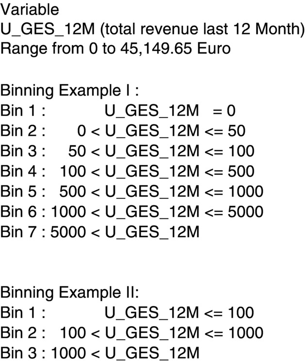
Figure 4.9 Dealing with binning.

Figure 4.10 Dealing with sextiles.
The standard programme selects the relevant variables from the meta-data with the help of a macro (i.e. a user-provided set of instructions). Then the Procedure (Proc) Univariate is carried out for these variables twice: firstly, for the general analysis of the single variables and, secondly, to determine the borders of the sextiles. The results, that is, the borders, pass into a programme step which independently generates a programme code and exports it, with the eventual outcome that we obtain a file with the classified variables (see Figure 4.11).
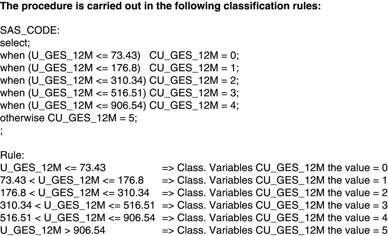
Figure 4.11 Classification rules.
After the data preparation and transfers are done, you can do the planned further analytical steps. If you like to solve prediction problems, it may help if you will have a feature reduction step before you conclude with the predictions.
4.9 Timing Considerations
Considerable time needs to be allowed for data preparation. As can be seen from the sections earlier, there are many different things to be aware of and steps to be taken. In common with most projects, time spent on preparation is seldom wasted.
The time needed for data preparation depends not only on the data but also on the experience of the practitioner. A more experienced data miner will need less time than a novice. It requires programming skills and familiarity with data preparation tools. Coded data can usually be prepared more quickly. Data preparation can take one to two days up to two to three weeks. In case the data structure is not clear, never estimate less than a week preparation time. Thereafter, the data may be in use for a long period.
Another issue is whether you have access to the data and whether you have all the necessary authorisation or have to ask other people to do things for you. It is quicker if you can do it yourself providing you are experienced. If you are not experienced, it may be better to have someone else do the data preparation for you.
Data is dynamic and frequently updated. In some cases, the data needs to be re-prepared weekly before it can be used.
4.10 Operational Issues
It is vital that the analyst realises the importance of understanding the definitions that the company uses. It should be noted that often the company may not have agreement on this within themselves. Whatever definitions the analyst uses, their results have to be compatible with those used in the marketing and customer relationship management reports. For example, does average age include missing values as zero or not, and are missing values included in the analytics or not? If zeros are included, a quantity like average age will end up being much lower than it is known to be. One way to check such important details is to map the analytical results to those in other business reports.