9
Intra-Customer Analysis
The following recipes describe how to make the best of customer information whether in a data mart fed from a data warehouse or from a more ad hoc data source. Descriptive analytics can derive rich information. We consider the use of cluster analysis and association rules as well as decision trees, logistic regression and Self-Organising Maps (SOMs).
9.1 Recipe 10: To Find the Optimal Amount of Single Communication to Activate One Customer
This is a descriptive analytics problem. The data collected by the client will be used to find hidden relationships between the variables and the buying behaviour of the client. It is not so necessary to have fine detail in the variables that are likely to be of major importance when we are just looking at the general relationship between the variables and the buying behaviour. Therefore, the variables have been put through the binning process, and the descriptive analysis proceeds with the binned values. The work in this chapter also relates to Recipe 1 (see Figure 9.1 ).
Figure 9.1 Activating customers.
Input data – must-haves: The recipe requires the full communication history and the buying history.
Target variables: The following could be useful as target variables: number and quantity of purchases or being active or not.
Data mining methods: Suitable descriptive methods include:
- Histograms and multiple bar charts
- Contingency tables and chi-square analysis
- Scatterplots and correlation
We could plot the response for different numbers and types of communication.
The binning and the analysis of relationships between variables and buying behaviour help to clarify how to find the optimal amount of single communication to activate one customer.
9.2 Recipe 11: To Find the Optimal Communication Mix to Activate One Customer
Industry: The recipe is relevant to everybody using direct communication to improve business, for example, mail-order businesses, publishers, online shops, department stores or supermarkets (with loyalty cards).
Areas of interest: The recipe is relevant to marketing, sales and online promotions.
Challenge: The challenge is to find the right combination of direct communications to activate a customer. Initially, as always, we will have a business briefing to determine exactly what is required.
In marketing, you have the problem that you are never totally sure what kind of campaign or combination of campaigns is successful. If you talk to experienced marketing colleagues, they will tell you that you need to build up awareness by communication to get reactions. This means that it is not only the last communication that is responsible for the reaction, but it is the combination of all previous communications. For example, a clothing manufacturer may have carried out the following combination of marketing activities over the last half-year: vouchers sent to selected customers, recommend a friend, buy one get one free and then finally they will get a reaction.
There are different ways to determine the optimal combination of communications:
- Describe the problem so that it can be treated as a prediction problem. The challenge here is to describe the target. After that, you can work in an analogous way to Recipes in Chapter 8.
- Use sequence and association rules to find and describe the patterns.
We will describe the use of sequence and association rules to solve this problem (see Figure 9.2 ).
Figure 9.2 Communications sent to activate a customer.
Population: The population is defined according to the actual problem and the briefing. It has to be discussed whether you include all customers (active and inactive) or just those who are currently active or who have only been inactive for a short while in the past. Note that inactive customers will still have received some kind of advertisement and that some of them may become active later on.
Depending on the number of customers, it might be useful to carry out sampling. If you decide to sample, the sampling has to be carried out on the customers and not on the records of advertisements or other promotional activities. You need to get a sample of customers and add all relevant data to them. Note that the distribution of the customers in the sample should be similar to that in the actual population so that the learning is representative of the actual data. The representativeness of the sample should be checked, and if necessary, some changes should be made. For example, a training sample was found to have more people in the working class than appear in the actual data. The sample was modified by taking a better stratified sample, and the model was rebuilt. Note that the population of interest may well be a subset of the whole customer database. We may also decide to further sub-divide if we think that different sequences and associations are likely with different groupings.
Necessary data: The areas of data that could be used must contain information on all kinds of advertisements and campaigns that could reach a customer and on the general customer reaction not only their direct response to one advert or communication.
Target variable: We do not have a target in the traditional way. The objective is more about trying to control and learn. The instructions will differ depending on the data mining software you use, for example, with SAS Enterprise Miner if we are looking for patterns of communication, then we will need to nominate the type of communication as the “target variable”.
Input data – must-have: This includes the following:
- Raw data on historical reactions to previous marketing activities, for example, the customer recommended a friend to a publisher, or returned a questionnaire, or used a voucher, in between the relevant time.
- Raw data on historical purchasing behaviour not just in response to previous campaigns, if any, but general historical behaviour. We include full details, for example, date, kind of product, amount, value and reductions in between the relevant time.
- Raw data of the historical details of advertisements, promotions and other communications sent to the customer.
- Raw data on all complaints that are not related to the buying process itself, for example, asking for status of commitment in terms such as ‘when can I stop my contract?’.
Example: The first few lines of typical data showing the input data (to be extended in the transformation section) are shown in Figure 9.3 .
Figure 9.3 Typical data about communications.
Data mining methods: The following methods can be used:
- Sequence analysis
- Association rules
How to do it:
Data preparation: The main issue is that after all the steps of transformation and aggregation have been done, you should have several (at least three) rows for every case (customer). Therefore, the data is in customer order with multiple rows for each customer.
Business issues: Before you start the next steps, think about the potential implementation. Any step/manipulation that you know will not be possible to do under implementation should not be used in the learning phase. It is very likely that the results will be used to guide future marketing campaigns automatically, so note that you must be able to implement the rules in your campaign management system.
Transformations: Based on the fact that things, that did not happen, are not stored in the database, you have to think how to create dummy cases that represent this ‘Nothing happened in a special time slot’ issue. ‘Nothing happened’ has two sides: no marketing and no customer reaction. The length of an average time slot in month, weeks, days or hours depends on your business and has to be discovered in the pre-analytics phase. If you, for example, detect that a week as a time slot will suit your business, you have to create a dummy variable for every week without advertisement or campaign and for every week without a customer reaction. Advertisements have to be classified into sub-groups such as standalone emailing, telephone marketing, direct mail, catalogue and salesman. Customer reaction has to be classified as well, for example, order, complaint, unsubscribe and return. Every case in the dataset should have an order number, if possible a date, the object and a customer ID.
Analytics:
Pre-analytics: As described earlier, you should use this pre-analytics stage to detect the right length of your ‘nothing happened’ slots and to control whether the chosen aggregation of your objects is at the right level.
Model building: We recommend the use of a sequence analysis because in the marketing context, the given order of objects is an important feature of the pattern. If the aggregation level of your observations is too low (too coarse with too many issues combined), it may be that you do not find any patterns. It is also very likely that you will find a well-known pattern, because they are the results of defined marketing and communication processes. For example, if your company sends out an email acknowledgement after every online customer interaction, this pattern of response will be so dominant that it might hide other really unknown patterns. In this case, you should go back to the data transformation and try to solve the problem of patterns being hidden by bundling such process items together into one item.
Example rules found are:
Email and then telephone campaign gives 20% take-up
Mail campaign, then email and then invite-a-friend gives 23% take-up
This is for a general population; we may also want to explore the rules when only men are included or just older people.
Evaluation and validation: Use the set of rules found on the test and validation samples and compare the observed results with the expected ones. We might compare the rules via the support and the confidence as described in the methods section.
An important question is whether the rules found fit with the business. If there are rules and patterns in the model that we cannot understand, and neither you nor anyone else knows why they are there, this suggests that the model is over-fitted and something is wrong with it.
We also have to look for special effects which show up via the model which we were not aware of or we had underestimated or forgotten. These could be specific to particular features, for example, something which only occurred in one year, or an abnormal reduction in the amount of advertising in a past year. Is the model useful for the business? Usefulness is judged by use and continued use and outcome in terms of financial benefit (see Figure 9.4 ).
Figure 9.4 Communication mix to activate a customer.
Implementation: The implementation can be done shortly after learning, or it is also possible to implement rules regularly like every week on new data to run fully automated campaigns.
It is necessary to do every single aggregation and transformation for all variables that are part of the rules.
Hints and tips: If possible, make sure that you can show and prove the quality of your model by comparing the results obtained with and without the model. For example, it is a good idea not to use your model to select 100% of the people who will be contacted (or get the marketing treatment) but to allow some of them to be selected in other ways which could be the original method used before.
You can then keep a check on the performance of your model and show its superiority by comparing the average responses. If you are confident in your model, you could let as many as 90% of the customers be chosen by the model and 10% be chosen in other ways. Otherwise, in the early days of adopting modelling, you could select 50:50. Note that another way of allowing this comparison is to split the population in the required ratio and make the selection from each part.
There are other good reasons for making only part of the selection by the model. One of these is to ensure that you do not lose the opportunity to observe the reaction of a group of people who are not considered important in the model but do exist in the population. Making part of the selection completely at random ensures that you have a sub-sample whose responses you can observe. For example, if the model indicates that gender is important, then you could end up with only females being selected, and in the future, no one would know how men react. Also, there would be no way to illustrate the success of your model without the reaction of some men to compare it with. Finally, you need to keep the variety in the customer selection so that when models are updated, there is a chance to pick up features that may have changed their importance.
Note that sometimes management will want to use the model for 100% of the selection because they believe it is the most cost-effective method, and unless you can persuade them otherwise, you will not be able to make the comparison discussed earlier.
How to sell to management: From the point of view of management, the rules are good if they
- Save money, or
- Improve sales, or
- Increase customer loyalty
regardless of how good the rules are in a statistical sense. Show the management money instead of statistics and numbers. If you cannot prove that at least one of the benefits in the three bullet points applies, then your rules might not be used. In any case, show them that if the campaigns do not follow your rules, they will waste money because they will need more marketing budget and more campaigns to be done more often.
9.3 Recipe 12: To Find and Describe Homogeneous Groups of Products
Industry: The recipe is relevant to everybody using data to learn and improve their product categories.
Areas of interest: The recipe is relevant to purchasing department, marketing, sales and online promotions.
Challenge: The challenge is to find the right combination of products to improve your category management. For example, this is important for department stores. There are two alternative ways to view the problem:
- The problem is about what is bought together – this kind of problem is solved by using association rules.
- The problem is about which products have similar usage and customers (a problem that will be solved by using clustering methods).
We will focus on the second option (see Figure 9.5 ).
Figure 9.5 Typical application of cluster analysis.
Necessary data: The data must contain detailed information on buying habits and customer demographics. Information on advertisements is nice to have but is not that necessary.
Population: Note that in this recipe the products are the cases rather than the customers, so it is the products that make up the population. If you have no other information, it might be useful to define all products that are offered in one year as the population.
You have to decide on what level of detail you want to envisage a product as a product. For example, consider the following situation:
Your company sells shirts and it is up to the product manager to decide on which level the product is seen as a product. Note that the customer may have a different view to the product manager.
There are different ways to describe shirts within the data; the following are a few options to help you visualise the situation:
Option 1
- Shirt, white, button-down-collar, long sleeves, buttons/no cuffs, size 17: product ID 140032 amount 1
- Shirt, white, button-down-collar, long sleeves, buttons/no cuffs, size 15: product ID 140029 amount 1
- Shirt, blue, button-down-collar, long sleeves, buttons/no cuffs, size 17: product ID 140056 amount 1
In option 1, there are three different products.
Or
Option 2
- Shirt, white, button-down-collar, long sleeves, buttons/no cuffs, amount 2
- Shirt, blue, button-down-collar, long sleeves, buttons/no cuffs, amount 1
In option 2, there are two different products.
Or
Option 3
- Shirt, button-down-collar, long sleeves, buttons/no cuffs, size 17, amount 2
- Shirt, button-down-collar, long sleeves, buttons/no cuffs, size 15, amount 1
In option 3, there are two different products.
Or
Option 4
- Shirt, button-down-collar, long sleeves, buttons/no cuffs, amount 3
In option 4, there is just one product.
- You have to use your domain knowledge to decide which level will help to solve the problem. The nature and significance of the potential results are influenced by it.
Target variable: There is no target as we are dealing with a method of unsupervised learning.
Input data – must-have: The must-have data includes:
- Raw data on historical reactions to previous marketing activities, for example, the customer recommended a friend to an outlet, or returned a questionnaire, or used a voucher, within the relevant time.
- Raw data on historical purchasing behaviour not just to the previous campaigns, if any, but general historical behaviour. We include full details, for example, date, kind of product, amount, value and discounts within the relevant time.
- Raw data of the historical details of advertisements, promotions and other communications sent to the customer.
- Raw data on all complaints that are not related to the buying process itself, for example, asking for status of commitment in terms such as ‘when can I stop my contract?’
Data mining methods:
- Cluster analysis
- SOMs
How to do it:
Data preparation: In this example, the products are the cases. So when you start generating the data, keep in mind that you have to build up everything from the viewpoint of the product. But generally, this is not a problem, and you can use the same ideas as would usually be used when dealing with customers but make sure it is from the product viewpoint.
Business issues: Before you start the next step, think of the potential implementation. Any step or manipulation that you know cannot be done in implementation should not be used in the learning phase. It is very likely that the result will be used for decisions and strategic planning, rather than for immediate practice, so the technical considerations of the implementation might be minor.
Whether you work on the level of a detailed product number or on an aggregated level depends on your actual briefing. If in doubt, it is better to be more detailed. But the detail level must be viewed from the customer usage viewpoint and not from the supply chain viewpoint, where two products that are absolutely similar may get two product numbers because they are produced by different companies.
Transformations: As in other modelling questions (e.g. in Chapter 8), the same kind of transformations and aggregations should be done, but the cases are products so you have to modify it a little bit.
Analytics:
Pre-analytics: You should use this phase to control whether the chosen aggregation of your objects is on the right level and to get a descriptive overview of the special aspects and descriptions of the products. Depending on the number of variables created, this phase can be used to detect those variables that might have some impact on the clustering.
Model building: We recommend using a hierarchical cluster method. The dendrogram might help you to explain the results more easily.
Evaluation and validation: Use the set of cluster descriptions found from the training samples and compare them with those found from the test samples.
Do the rules found fit with the business? If there are rules and patterns in the model that we cannot understand, and neither you nor anyone else knows why they are there, this suggests that the model is over-fitted and something is wrong with it.
We also have to look for special effects which show up via the model which we were not aware of or we had underestimated or forgotten. These could be specific to particular features, for example, which only occurred in one year, for example, like a special ‘birthday offer’. Sometimes, it is better to delete these products from the dataset and to redo the analysis.
Finally, you have to check whether the model is useful for the business.
Implementation: The results are mostly used for strategic decisions, so there are no technical barriers to be aware of.
Hints and tips: If you get the impression that the results seem to be a bit boring or peculiar, try a different kind of aggregation level for the product. Make sure that product numbers are unique or a historical dimension table for additional product information is available. Make sure that, for example, socks and washing machines do not share the same product number: for example, until 30 August 2010 (product ID 12345, socks) and from 1 September 2010 to 31 July 2011 (product ID 12345, washing machine). These things do happen!
How to sell to management: Include a graphic, for example, a dendrogram or other visualisation. Also, you can shorten the cluster descriptions and present them as a profile.
9.4 Recipe 13: To Find and Describe Groups of Customers with Homogeneous Usage
In general, this recipe is a variation of Recipe 12. Recipe 12 is about products and Recipe 13 is about customers, so on one level you can just say that the objects are turned round. But handling single customers as a single line in datasets might give you more opportunities to add data at different levels of aggregation. So it seems to be a good idea to dedicate a recipe to this situation and to go into some detail.
Industry: The recipe is relevant to all sectors.
Areas of interest: The recipe is relevant to marketing, sales and strategic decisions.
Challenge: The challenge is that marketing as well as sales needs to have a more tangible picture or description of different customer or consumer groups. To provide these group descriptions, different solutions can be chosen:
- Segmentation can be carried out by drawing on knowledge of the business and experience. For example, the segmentation may be based on gender, fixed age groups (like 18–24, 25–34, 35–44), etc.
- Advantage: Segmentation can be done easily, only limited statistical knowledge is necessary, and it is easy to explain to marketing managers. Also, it fits in with any pre-existing prejudices.
- Disadvantage: There is less chance to find unforeseen results and new knowledge; because the experiences are often not specific to a single company, it is very likely that you end up with the same segments as your competitor.
- Segmentation can be carried out using a data-driven approach: the segmentation is based on statistical algorithms that try to find groups of customers with homogeneous behaviours.
- Advantage: There is good chance to find new target groups that were not obvious or easy to find. It is possible to find patterns that are specific only for this company, for example, target groups sharing the same age and gender but with very different behaviour. This group can now be separated from the others on the basis of this behaviour.
- Disadvantage: There is a need for statistical knowledge and statistical software. The ability to sell the results to marketing managers must also be very high.
Necessary data: The areas of data that could be used must contain information on all kinds of buying behaviour of single customers, advertisements and campaigns that could reach a customer and the general customer attributes.
Population: This is defined according to the actual problem and the business briefing. It has to be discussed whether you include all customers including active and inactive ones or not. In general, you need a splitting criterion for the segments that is not used to define the population used to learn on. So, for example, if we have used active and non-active customers to split up the population, then we cannot use ‘general activity’ as a criterion for the segmentation for either group because everyone has the same score for that variable.
Note that in cluster analysis, we have to reduce the population size; otherwise, the computational time becomes too large. We can reduce the population size either by using a splitting criterion such as gender or activity level or by random sampling. If we use random sampling, an important variable like gender or activity level is likely to dominate the clusters so that one cluster just contains the people in one part of the splitting criterion, and this is not a particularly useful outcome. Therefore, it is often more useful to use a splitting criterion to reduce the population size and produce two or more cluster analyses, one for each part of the splitting criterion.
Target variable: As we are dealing with an unsupervised learning problem, no target is needed.
Input data – must-haves: The must-have data includes:
- Raw data on historical reactions to previous marketing activities, for example, the customer recommended a friend to a publisher, or returned a questionnaire, or used a voucher.
- Raw data on historical purchasing behaviour not just to previous campaigns, if any, but general historical behaviour. We include full details such as date, kind of product, amount, value, channel of purchasing, for example, online shop or local shop, salesperson and reductions such as buy one get one free.
- Raw data of the historical details of advertisements, promotions, visits by salesman and other communications sent to the customer.
- Cost per customer for every marketing and sales activity (marketing costs).
- Cost/margin for products.
- General customer attributes such as gender, age, occupation, salary and education.
Data mining methods:
- Frequency and mean values
- Clustering
- SOMs
How to do it:
Data preparation: In this example, the customers are the cases. In a similar way to other recipes, it is necessary to aggregate and transform the raw data. You should follow the rule of having one line of information storing several variables per individual customer. It is possible to use data marts that have the data in a suitable format.
Depending on the number of customers who are available, a sample is a good solution. For example, if your database contains 1.5 million customers, this number might be too large to get a clustering result back from the computer in a reasonable work time, so it is a good solution just to learn on a sample of maybe 30 000 customers. The number of variables should be limited according to business considerations, aggregation and the fact that most of the clustering algorithms can only handle a given number of variables to calculate the clusters.
Business issues: It is very likely that the results will be used as a first step for decision making and strategic planning, so the technical considerations regarding the implementation might be small in the beginning. But nevertheless, there might be a need to mark a single customer with the cluster number of the cluster they belong to, and so this should be done in readiness. Before you start the next steps, think about the potential implementation. Any step or manipulation that you know cannot be done when you implement the rules or cluster definitions should not be used in the learning phase.
Transformations: As always with modelling, the same kind of transformations and aggregation should be done to generate the variables that can be used in the cluster algorithm.
Analytics: We consider the three alternatives:
Experience-based approach of segmentation: To carry out this approach, first set up the rules for the experience-based segments, for example, one segment may be women aged 18–34 years old. Then group people in different segments with all their associated datasets and variables.
An example of potential segments is shown in Figure 9.6 .
Figure 9.6 Example of segments.
This approach uses frequency, ranks and means to calculate numbers that might help to describe the segment and its behaviour in detail. Some examples are:
- Number of people in the individual segment
- % of total customers
- Average revenue last year
- Average revenue in total
- Three most relevant products
- Three most common occupations
- Three most common residences
- % of people with Single Sign-On (SSO) Registration
- Most relevant social network
- …
The question of the kind of numbers that are relevant depends on the individual business task and available information. The numbers add to the clarification as shown in Figure 9.7 .

Figure 9.7 Potential ways to present a cluster (named Lea).
Data-driven approach of segmentation: This approach uses cluster algorithms or SOMs. Several algorithms are implemented in data mining tools. Before using them, it is important to check which size of dataset will operate or if there are any given limitations. Based on that restriction, it might be useful to reduce the original dataset by sampling and to reduce the variables to those which might be potentially used in the cluster description that will be presented to the management board. A hint of which kind of variables might be more relevant to separate different groups of customers can also be generated by a closer look at the list of important variables given in a predictive modelling project that you or one of your colleagues might have done before.
As a rule of thumb, the dataset should contain fewer than 40 000 rows and fewer than 250 variables to reduce the calculation time of the algorithm to a reasonable size. But with increasing computer power, this limit might expand.
In general, it is recommended to use the default settings of the data mining tool to start the clustering, especially if you do not have any prior knowledge on the amount of potentially existing clusters or other knowledge that might be useful to speed up the process.
Evaluation and validation: Based on the fact that cluster algorithms belong to the group of unsupervised learning, there is no additional process of validation than the check points delivered by the data mining tool. But nevertheless, it is still important to cross-check the results according to whether they make good business sense.
Implementation: Both kinds of segmentation can be implemented on really big amounts of data just by using the defined or detected rules:
For the experience-based approach, it is quite easy – just use the definitions that are used to build the segments.
For the data-driven approach, it is a little bit more complicated: If you can use an application function in your data mining tool that allows you to use a different dataset for the application than the one for training, it is quite easy. Just make sure that the new dataset includes the same variables and that the variable measurement is similar to that in the learning dataset; then it is possible to mark the dataset with cluster membership so that each customer is allocated to one of the detected segments.
In case your data mining tool does not provide such a function, then you have to work out the rules of implementation yourself. There are two different approaches: one is to generate the rules and the other is to develop the predictive models for each segment.
To generate rules, calculate the mean for each continuous variable in each segment and its accompanying confidence interval; for categorical variables, find the most common category in each segment. Then construct a set of rules to decide which segment to allocate each customer to. An example of these rules is as follows:
For each customer, if age is within the confidence interval for segment 1 and if the gender is in the modal category and if the home address is in the modal region, then allocate the customer to segment 1.
Clearly, this ad hoc approach can lead to some customers fitting into a number of different segments and other customers not fitting into any segments. The practical solution is to omit customers without a segment and allocate customers with multiple options to one segment at random. This is a pragmatic approach, and so if there are a lot of segment-less customers, then the process of allocation has to be repeated with wider confidence intervals.
If there are a lot of important variables defining the clusters, then the predictive model approach is recommended. To do the predictive modelling, work with the sample that was used for the cluster analysis and create a binary target variable which is 1 for segment 1 members and 0 for everyone else. Then create the model using the important variables from the cluster analysis. You can then apply the predictive model to the whole population and obtain a probability of having target = 1 for each customer. The process is repeated for each segment. We now have a set of probabilities of segment membership, one for each segment, and we can allocate the customer to the segment for which they have the highest probability of membership. Usually, this works well and may be faster than trying to generate rules that discriminate successfully.
Most of the time, an application on all (or new) data is not necessary, because the cluster results are just used strategically and for planning purposes. It helps to sell the results to management if meaningful names are worked out for each cluster, for example, young professionals or retired people.
9.5 Recipe 14: To Predict the Order Size of Single Products or Product Groups
This problem can be solved as a predictive model. You can follow the recipes in Chapter 8 in general but with some amendments.
Target variable: Instead of the target being a binary variable (whether the customer responded to a particular offer or not), in this recipe, the target will be continuous or at least categorical. The target variable represents an aggregation of buying behaviour. You have to decide whether a detailed (continuous) target will add a real business benefit or not. If it is more important for the business to know whether a customer is likely to buy ‘a few’ items of a specific product than it is to predict the exact number, then the target should be classified into a categorical variable rather than being a continuous variable.
Data mining methods: If you decide to have the target as a continuous variable, then you can use multiple linear regression or another method suitable for a continuous target. If the target is classified, then logistic regression analysis can be used or you can develop separate models for each class as in Chapter 8.
Transformations: We strongly recommend that the input variables are transformed as described in Chapter 8. Using the binning or quantile methods helps to stabilise the models, especially if the environment where the input data is collected is constantly changing or if the data is collected directly from a legacy system. As a rule of thumb to decide whether the input data should be transformed to a classified variable or to keep it continuous, if it is a common pattern in your data that mean and median differ a lot, then classification of the input variables is recommended to keep the model more stable.
Implementation: If the target is classified, then you can develop a model for each class (just following Chapter 8). Each of these ‘class’ models should be deployed on the customers, and, for each customer, the model that gives the highest score wins (see Figure 9.8 ).
Figure 9.8 Example showing scores for different models.
Notice that it is not always absolutely clear which model wins. For the last customer in the table, customer ID 2378, the only thing you can say is that it is likely that the person will buy in general and that it might be more than six items.
9.6 Recipe 15: Product Set Combination
This recipe is a common variation of Recipe 11. The target has changed from communication channels to products. The central issue is the definition of the product. It does not sound as if it is a big problem, but it can be quite difficult depending upon your point of view. Consider the following definitions with reference to Figure 9.9 and the different viewpoints:
- Logistic/warehouse: Each bottle has its own product ID and storage place in the warehouse. ⇒10 different products
- Sales and marketing: Each bottle has its own product ID. It may belong to different brands, have a different size and a different price. ⇒10 different products
- Customers: It is mineral water but customers may differentiate between natural and sparkling or between brands or between price levels. ⇒So the number of products depends on the context and how a customer might see the product; therefore, it could be from 1 product to 10 products.
Figure 9.9 Ten bottles of water, all the same?
From the point of view of analytics, you should decide on the aggregation level (product ID) to reflect the customer view depending on the business aspects, the available data and the goal that should be reached by the analytics.
It might be useful to do the analysis at least twice: First time to analyse on a highly aggregated level like ‘mineral water’, ‘beef’, ‘vegetables’, ‘sweets’, ‘cereals’ and ‘soft drinks’. This helps to find out what the common combinations are and how big they are in total. Support and confidence are good indicators of the importance of the combinations as well. For the second time to analyse on a different level, for example,
- Mineral water: Sparkling and natural
- Versus
- Beef: Neck, chuck, brisket, flank, rib, sirloin, tenderloin, top, round and shank
- Versus
- Vegetable: Mushrooms, carrots, spinach, peas, eggplant, tomatoes, potatoes and beans
As you may appreciate, the number of combinations increases dramatically and each potential combination might be small, or the support and confidence may be too small to indicate a trustable product setup.
So the most difficult issue in this recipe is to decide on the right level of aggregation of the products to generate stable results on the one hand and detailed level usable results on the other. A higher level of aggregation is better for generalisation because it is very likely that product details may change.
9.7 Recipe 16: To Predict the Future Customer Lifetime Value of a Customer
Industry: The recipe is relevant to all sectors.
Areas of interest: The recipe is relevant to strategic decisions, marketing, sales and control.
Challenge: Calculating the Customer Lifetime Value (CLV) at the level of existing customers or addresses known in the past is a common activity. However, the challenge here is to include a prediction of future customer behaviour. The prediction of future customer value makes all the difference because only this guides you to the right strategic decisions in customer development. The traditional way of using past data could mislead because it just deals with the past behaviour and does not include the potential forthcoming behaviour of the customer (see Figure 9.10 ).
Figure 9.10 CLV development.
So the challenge is to calculate the future value of a customer by combining the results of a prediction model that predicts the future affinity to order or not to churn (if you are in the subscription business) and traditional CLV models. So we have to do two steps: first work out a predictive model that enables us to estimate the future behaviour of a single customer, and secondly based on the prediction, we calculate the net present value for each single customer. As an example, consider the case where you have to predict the affinity to order; suppose you are a producer of machines for craftsmen and you sell directly via a catalogue, online shop and salesmen.
Necessary data: The areas of data that could be used must contain information on all kinds of advertisement and campaigns that could reach a customer including all associated costs and the general customer reaction not just the direct response to one advert or communication.
Population: The population is defined according to the actual problem and the business briefing. It has to be discussed whether you include all customers including active and inactive ones or not. If for older and inactive customers the data and especially the cost information are unavailable and cannot be estimated, it is better to concentrate on the active customers.
Target variable: The target is a binary variable such as ‘buying’ or ‘not buying’ in a specific time slot. For some companies especially in B2B, it makes sense to count successful recommendations as Target = 1 as well.
Input data – must-have: Must-have data includes:
- Raw data on historical reactions to previous marketing activities, for example, the customer recommended a friend to a publisher, or returned a questionnaire, or used a voucher.
- Raw data on historical purchasing behaviour not just to previous campaigns, if any, but general historical behaviour. We include full details such as date, kind of product, amount, value, channel of purchasing, for example, online shop, local shop, salesperson and reductions, for example, buy one get one free.
- Raw data of the historical details of advertisements, promotions, visits by salesman and other communications sent to the customer.
- Cost per customer for every marketing and sales activity (marketing costs).
- Cost/margin for products.
- General cost per customer for handling.
- Try to get the information as complete as possible; if some information is only available on a general level, try to break it down to customer level.
Data mining methods:
- A simple prediction of future buying behaviour (e.g. time series model).
-
CLV calculation: In the simplest form, the net present value method can be used to determine the lifetime value. In this method, values are input for the expected customer proceeds, et (based on sales, cross-selling revenue, etc.), and the customer-specific costs, at (mailings, advice, investment, etc.), for each time period, t, in the expected duration, T, of the relationship. The costs are subtracted from the proceeds and discounted using a discount rate, i, and then summed over all the time periods:
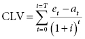
How to do it:
Data preparation: In this example, the customers are the cases and you just try to summarise both objects et and at for each time period t.
Business issues: Before you start the next steps, think about the potential implementation. Any step or manipulation that you know cannot be done when you implement should not be used in the learning phase.
It is very likely that the result will be used as a first step for decisions and strategic planning, so the technical considerations regarding the implementation might be small in the beginning. But note if the CLV-based strategies are implemented, there is an upcoming need to do the CLV calculations fully automatically and regularly.
Transformations: As in other predictive modelling questions, the same kind of transformations and aggregation should be done to generate the customised proceeds and costs for each past time period.
Analytics:
Pre-analytics: You should use this phase to control whether the chosen aggregation of your objects should be the customers or customer groupings or the way that purchases are accounted for. For example, should purchases made in the morning or in the afternoon count as being in the same day or should another system be used where a purchase is only counted when it is paid for? So at this stage, it is important to check that your numbers are all fitting in the same reporting universe, in other words that you have sound operational definitions.
Model building: The CLV for each customer is calculated using the formula provided earlier. For each customer, start with their individual setup costs from the time they began their business relationship with you. Then calculate costs and proceeds for all periods with real numbers out of the system. In many cases, a year is a suitable time period, t. Usually, data is used for each year that the customer was in the relationship with the company, which could be before they actually purchase if there is a long lead in, for example, companies selling cars, houses or new kitchens.
At the end, you will get the actual CLV without the forecasting aspect. The cost or profit of the customer is just added to the company’s business results. Even if you stop here, these results already have great value for your company and will help to improve your CRM strategies.
For the prediction of the future customer behaviour, we recommend using a time series model based on revenue and advertisements over the past time periods. To get a result for the potential and expected future CLV of each single customer, you should use the estimated values in the formula for each future point in time. In most business areas, a forecast of three to five years ahead is fine.
Note that a 70-year-old will have a greater CLV than a 35-year-old but may not be such a good future customer. Factors such as biological age, however, may not have such a great impact if the forecast period is short. The impact will also vary with product, for example, age is unlikely to impact on buying food but may impact on investment purchases. Changes in costs and proceeds over time will be part of the variation in the data used in the time series modelling and so should carry through into the forecasts. However, it is also possible to incorporate explanatory variables explicitly in time series modelling. Note that a good customer may not necessarily remain good (see Figure 9.11 ).
Figure 9.11 CLV development. Note that good today may not be good tomorrow.
Evaluation and validation: We need to check both the prediction model and the calculated CLV. Apart from making sure that your calculation is correct on a technical level, the only way to validate the models is to cross-check the results with figures from other reports (your own and those of any other companies that you can find) to see whether the types of people that you predict will be valuable customers usually turn out so to be.
Do the rules of the time series models fit with the business rules? If there are rules and patterns in the model that we cannot understand, and neither you nor anyone else knows why they are there, this suggests that the model is over-fitted and something is wrong with it. Apart from cross-checking with other numbers, no additional validation of the whole CLV is necessary.
Implementation: There are two particularly important points to note:
The results are mostly used for strategic decision so there are no technical barriers to be aware of.
In case the algorithm is implemented, make sure that it enables you to replace the forecast by real numbers in the model and do a new forecast after the period is over.
Hints and tips: You will get the CLV for customers as a continuous value. Additionally, you should group the CLV into classes with the help of statistical or business rules. For example, the CLV for a particular customer may be 200 000 €, and overall the customers may have CLVs ranging from 10 000 to 2 million €. We would look at the frequency distribution to divide the customers up or use business rules developed over the history of the company from experience or from a wish list. For example, any customers with CLV over 1 million € may be counted as one category, or historically, they may be further grouped into a number of categories. Finally, we then end up with a table showing the % of customers with CLV in different categories.
How to sell to management: As a first step, it might be enough to include simple groupings of the CLV in the reports, for example, customers with a ‘big loss’, ‘small loss’, ‘hardly any balance (around zero)’, ‘small profit’ and ‘big profit’.
A good overview can be given by presenting the results in the form of a matrix with CLV categories on one axis and predictions on the other axis. In the so-called Boston matrix format, there are four groups in a 2 × 2 contingency table with high and low CLV in rows and high and low prediction in columns. Enter the numbers or % of customers in each part. The customers in the four parts of the table are: cash cows but no further development likely (high CLV, low prediction), rising stars with good value at present and good potential (high CLV, high prediction), uncertainties for whom we are not sure what will happen in the future (low CLV, high prediction) and poor dogs with no hope now and no hope of any improvement in the future (low CLV, low prediction). Such tables were originally used for market share and growth but are now used more widely.
We are calculating a CLV for each person so we can group the values by region and salesman or customer types or by association, for example, we can classify by use of hotel group or holiday type. This would indicate which other companies it is good to team up with.
You should note that the calculation of the CLV will start a major discussion in your company. In our example, it is very likely that it might have an influence on the management of the salesmen.