Chapter 7. Model Interpretability and Transparency with Automated ML
We discussed earlier how building good machine learning models is a pretty time-consuming process. What is a “good” machine learning model? We saw that this is usually defined by performance of the model, as measured by accuracy or similar metrics. As companies get ready to adopt machine learning for business-critical scenarios, interpretability and transparency of machine learning models becomes vital.
In this chapter, we cover key aspects around interpretability and transparency of machine learning that leads to customer trust. Interpretability and transparency become even more important when you are trying to use or customize a machine learning pipeline developed by others, including those generated by Automated Machine Learning systems. Let’s take a deeper look at how automated ML on Microsoft Azure Machine Learning enables model interpretability and transparency.
Model Interpretability
Most machine learning models are considered black boxes because it’s usually difficult to understand or explain how they work. Without this understanding, it is difficult to trust the model, and therefore difficult to convince executive stakeholders and customers of the business value of machine learning and machine learning–based systems.
Some models, like linear regression, are considered to be fairly straightforward and therefore easy to understand, but as we add more features or use more complicated machine learning models like neural networks, understanding them becomes more and more difficult. Usually, more complex (and not-so-easy-to-understand) models perform much better—that is, they achieve greater accuracy—than those that are simpler, and easier to understand. Figure 7-1 shows this relationship.
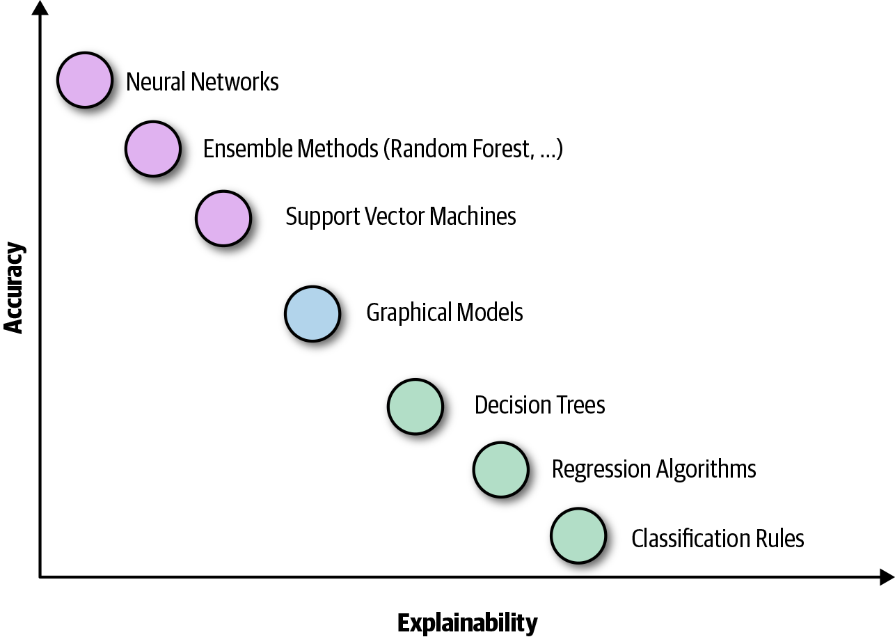
Figure 7-1. Interpretability/explainability versus model performance
Businesses run on transparency and trust, and being able to open the machine learning black box to explain a model helps build transparency and trust. In heavily regulated industries like health care and banking, interpretability and transparency are critical. Here are few real-world scenarios to illustrate the value of interpretability and transparency in machine learning:
-
A manufacturing company using machine learning to predict future instrument failure so that it can proactively perform maintenance activity.
-
When you know an instrument is about to fail, what’s the most likely cause going to be so that you can quickly perform preventive maintenance?
-
-
A financial institution using machine learning to process loan or credit card applications.
-
How do you know whether the model is doing the right thing?
-
If a customer asks for more details on why their application was rejected, how will you respond to them?
-
-
An online retailer or an independent software vendor (ISV) using machine learning to predict customer churn—in other words, whether a customer is going to stop using their product/service soon.
-
What are the key contributors to customer churn?
-
How can you prevent customers from churning?
-
Feature importance is a popular approach used for model interpretability. Feature importance indicates how each input column (or feature) affects the model’s predictions. This allows data scientists to explain the resulting model and predictions so that stakeholders can see which data points are most important in the model.
Model Interpretability with Azure Machine Learning
The Azure Machine Learning Python SDK offers various interpretability packages to help you understand feature importance. Using these packages, you can explain machine learning models globally on all data, or locally on a specific data point.
Explainers
There are two sets of explainers in the Azure Machine Learning SDK, specifically the azureml.explain.model package: direct explainers and meta explainers.
Direct explainers come from integrated libraries. A popular approach for explaining the output of machine learning model is SHAP (short for “SHapley Additive exPlanations”). The following is a list of the direct explainers available in the SDK:
- SHAP Tree Explainer
-
SHAP’s Tree Explainer focuses on trees and ensembles of trees.
- SHAP Deep Explainer
-
Based on the explanation from SHAP, Deep Explainer focuses on deep learning models. TensorFlow models and Keras models using the TensorFlow backend are supported (there is also preliminary support for PyTorch).
- SHAP Kernel Explainer
-
SHAP’s Kernel Explainer uses a specially weighted local linear regression to estimate SHAP values for any model.
- Mimic Explainer
-
Mimic Explainer is based on the idea of global surrogate models. A global surrogate model is an intrinsically interpretable model that is trained to approximate the predictions of a black-box model as accurately as possible. You can interpret a surrogate model to draw conclusions about the black-box model.
- PFI Explainer
-
Permutation Feature Importance (PFI) Explainer is a technique used to explain classification and regression models. At a high level, the way it works is by randomly shuffling data one feature at a time for the entire dataset and calculating how much the performance metric of interest decreases. The larger the change, the more important that feature is.
- LIME Explainer
-
Local interpretable model-agnostic explanations (LIME) Explainer uses the state-of-the-art LIME algorithm to create local surrogate models. Unlike the global surrogate models, LIME focuses on training local surrogate models to explain individual predictions. This is currently available in only the contrib/preview package
azureml.contrib.explain.model. - HAN Text Explainer
-
HAN Text Explainer uses a hierarchical attention network for getting model explanations from text data for a given black-box text model. This is currently available only in the contrib/preview package:
azureml.contrib.explain.model.
Meta explainers automatically select a suitable direct explainer and generate the best explanation information based on the given model and datasets. Currently, the following meta explainers are available in the Azure Machine Learning SDK:
- Tabular Explainer
- Text Explainer
- Image Explainer
Text Explainer and Image Explainer are currently available only in the contrib/preview package azureml.contrib.explain.model.
In addition to automatically selecting direct explainers, meta explainers develop additional features on top of the underlying libraries and improve the speed and scalability over the direct explainers. Currently TabularExplainer employs the following logic to invoke the direct explainers:
-
If it’s a tree-based model, apply
TreeExplainer, else -
If it’s a DNN model, apply
DeepExplainer, else -
Treat it as a black-box model and apply
KernelExplainer.
The intelligence built into TabularExplainer will become more sophisticated as more libraries are integrated into the SDK.
Figure 7-2 shows the relationship between direct and meta explainers and which ones are suitable for different types of data. The SDK wraps all of the explainers so that they expose a common API and output format.
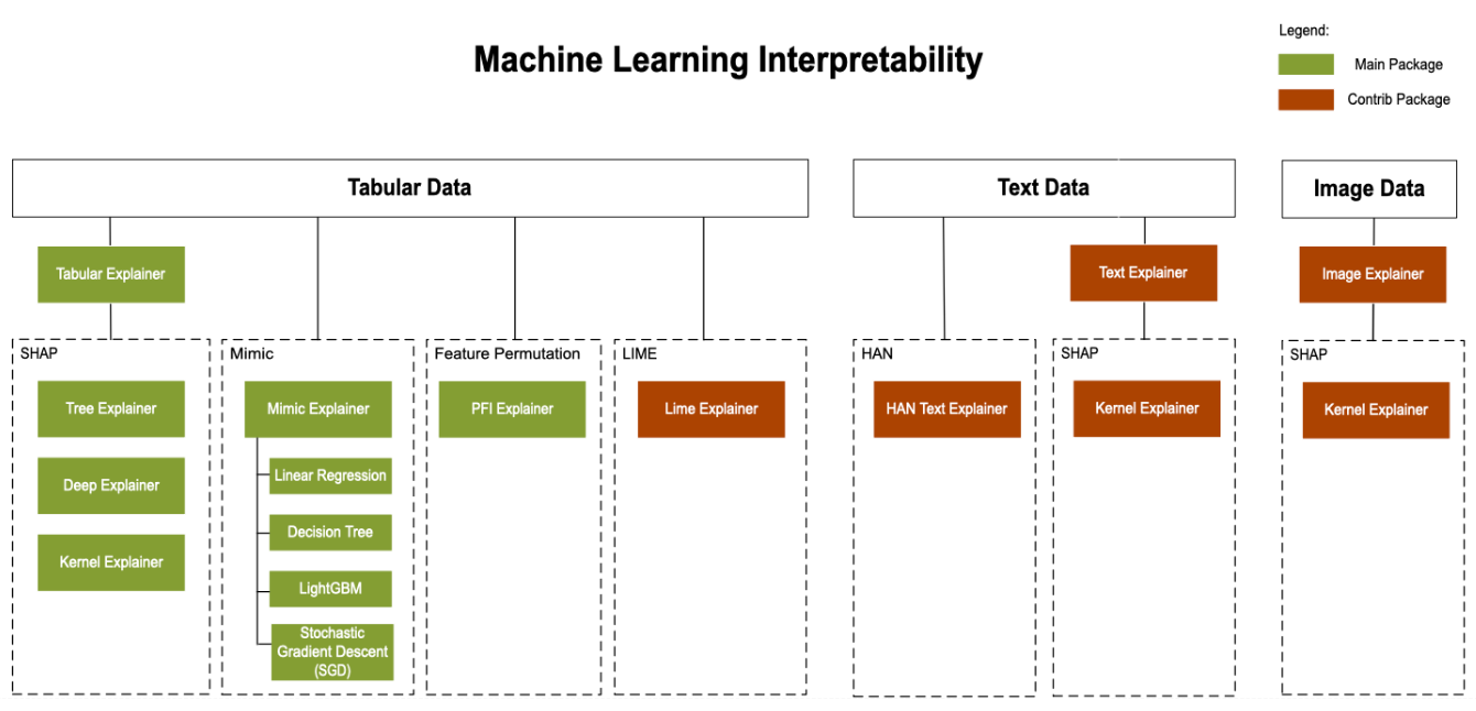
Figure 7-2. Direct and meta explainers
You’ll now see how to use these explainers in generating feature importance for the following two scenarios: a regression model trained using sklearn and a classification model trained using automated ML.
Regression model trained using sklearn
We will build a regression model to predict housing prices using the Boston house price dataset from sklearn. The dataset has 506 rows, 13 input columns (features), and 1 target column. Here are the input columns:
-
CRIM: Per capita crime rate by town
-
ZN: Proportion of residential land zoned for lots over 25,000 sq. ft.
-
INDUS: Proportion of nonretail business acres per town
-
CHAS: Charles River dummy variable (1 if tract bounds river; 0 otherwise)
-
NOX: Nitric oxides concentration (parts per 10 million)
-
RM: Average number of rooms per dwelling
-
AGE: Proportion of owner-occupied units built prior to 1940
-
DIS: Weighted distances to five Boston employment centers
-
RAD: Index of accessibility to radial highways
-
TAX: Full-value property-tax rate per $10,000
-
PTRATIO: Student-teacher ratio by town
-
B: 1,000 * (Bk–0.63)2, where Bk is the proportion of African Americans by town (this dataset is from 1978)
-
LSTAT: % lower status of the population
And this is the one target column:
-
MEDV: Median value of owner-occupied homes in $1,000s
After loading the dataset and splitting it into train and test sets, we train a simple regression model using sklearn GradientBoostingRegressor. Next we’ll use TabularExplainer from the azureml.explain.model package to generate global feature importance for the trained model. After the global explanations are generated, we use the methods get_ranked_global_values() and get_ranked_global_names() to get ranked feature importance values and the corresponding feature names:
fromsklearn.ensembleimportGradientBoostingRegressorreg=GradientBoostingRegressor(n_estimators=100,max_depth=4,learning_rate=0.1,loss='huber',random_state=1)model=reg.fit(x_train,y_train)fromazureml.explain.model.tabular_explainerimportTabularExplainertabular_explainer=TabularExplainer(model,x_train,features=boston_data.feature_names)global_explanation=tabular_explainer.explain_global(x_train)# Sorted SHAP values('Ranked global importance values:{}'.format(global_explanation.get_ranked_global_values()))# Corresponding feature names('Ranked global importance names:{}'.format(global_explanation.get_ranked_global_names()))# Display in an easy to understand formatdict(zip(global_explanation.get_ranked_global_names(),global_explanation.get_ranked_global_values()))
Figure 7-3 shows ranked global feature importance output. This indicates that the LSTAT (% lower status of the population) feature is most influential on the output of the model.
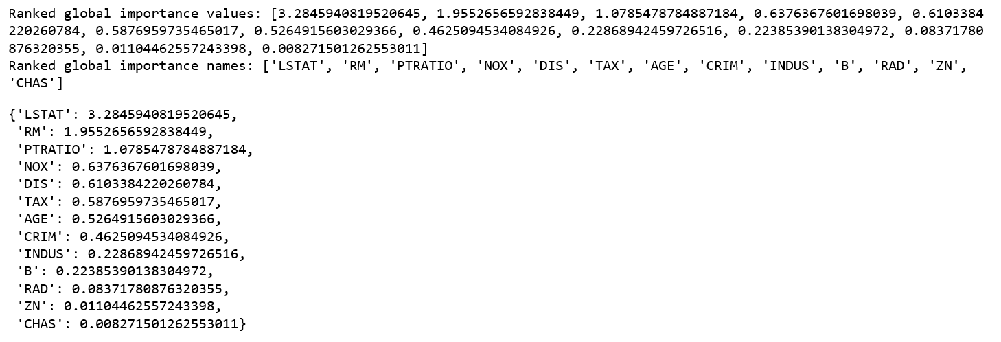
Figure 7-3. Global feature importance
Next, we look at how to compute local feature importance for a specific row of data. This is especially relevant at prediction time. We pass one row from the test set to explain_local() method and print the local feature importance:
local_explanation=tabular_explainer.explain_local(x_test[0,:])# Sorted local feature importance information; reflects original feature order('sorted local importance names:{}'.format(local_explanation.get_ranked_local_names()))('sorted local importance values:{}'.format(local_explanation.get_ranked_local_values()))# Display in an easy to understand formatdict(zip(local_explanation.get_ranked_local_names(),local_explanation.get_ranked_local_values()))
As seen in Figure 7-4, although LSTAT remains as the topmost feature in terms of importance for this specific test record, AGE is the second most impactful feature.

Figure 7-4. Local feature importance
As discussed in Chapter 4, raw data usually goes through multiple transformations before going through the training process. Features produced through this process are called engineered features, whereas the raw input columns are known as raw features. By default, explainers explain the model in terms of features used for training (i.e., engineered features) and not on the raw features.
However, in most real-world situations, you would like to understand raw feature importance. Raw feature importance informs you how each raw input column influences the model prediction, whereas engineered feature importance is not directly based on your inputs columns, but on columns generated through transformations on input columns. Hence, raw feature importance is a lot more understandable and actionable than engineered feature importance.
Using the SDK, you can pass your feature transformation pipeline to the explainer to receive raw feature importance. If you skip this, the explainer provides engineered feature importance. In general, any of the transformations on a single column will be supported:
fromsklearn.pipelineimportPipelinefromsklearn.imputeimportSimpleImputerfromsklearn.preprocessingimportStandardScaler,OneHotEncoderfromsklearn.linear_modelimportLogisticRegressionfromsklearn_pandasimportDataFrameMapper# Assume that we have created two arrays, numerical and categorical,thatholdthenumericalandcategoricalfeaturenames.numeric_transformations=[([f],Pipeline(steps=[('imputer',SimpleImputer(strategy='median')),('scaler',StandardScaler())]))forfinnumerical]categorical_transformations=[([f],OneHotEncoder(handle_unknown='ignore',sparse=False))forfincategorical]transformations=numeric_transformations+categorical_transformations# Append model to preprocessing pipeline.# Now we have a full prediction pipeline.clf=Pipeline(steps=[('preprocessor',DataFrameMapper(transformations)),('classifier',LogisticRegression(solver='lbfgs'))])# clf.steps[-1][1] returns the trained classification model# Pass transformation as an input to create the explanation object# "features" and "classes" fields are optionaltabular_explainer=TabularExplainer(clf.steps[-1][1],initialization_examples=x_train,features=dataset_feature_names,classes=dataset_classes,transformations=transformations)
So far, you have seen how to generate feature importance during model training time. It is also important to understand feature importance at inference time for a specific row of data. Let’s consider this scenario: suppose that you own a machine learning–powered application to do credit card application processing. If your application rejects a credit card application, you need to explain why the model rejects that specific applicant.
To enable inference-time feature importance, the explainer can be deployed along with the original model and can be used at scoring time to provide the local explanation information. Next, we examine how to enable feature importance with the automated ML tool in Azure Machine Learning.
Classification model trained using automated ML
We will use the sklearn iris dataset. This is a well-known classification scenario for flowers. There are three classes of flowers and four input features: petal length, petal width, sepal length, and sepal width. The dataset has 150 rows (50 rows per flower class).
After loading the dataset and splitting it into train and test sets, we train a classification model using automated ML. To enable feature importance for each of the models trained by automated ML, we set model_explainability=True in AutoMLConfig:
automl_config = AutoMLConfig(task = 'classification',
                             debug_log = 'automl_errors.log',
                             primary_metric = 'AUC_weighted',
                             iteration_timeout_minutes = 200,
                             iterations = 10,
                             verbosity = logging.INFO,
                             X = X_train,
                             y = y_train,
                             X_valid = X_test,
                             y_valid = y_test,
                             model_explainability=True,
                             path=project_folder)

local_run = experiment.submit(automl_config, show_output=True)

best_run, fitted_model = local_run.get_output()
Because this is a classification problem, you can get not only overall model-level feature importance, but also feature importance per class.
Let’s review how to use the azureml.train.automl.automlexplainer package to extract feature importance values from models generated in automated ML. We use the best run here as an example, but you can retrieve any run from automated ML training:
fromazureml.train.automl.automlexplainerimportretrieve_model_explanationshap_values,expected_values,overall_summary,overall_imp,per_class_summary,per_class_imp=\retrieve_model_explanation(best_run)# Global model level feature importance('Sorted global importance names: {}'.format(overall_imp))('Sorted global importance values: {}'.format(overall_summary))# Global class level feature importance('Sorted global class-level importance names: {}'.format(per_class_imp))('Sorted global class-level importance values:{}'.format(per_class_summary))
Figure 7-5 shows the output: global feature importance for the model and class-level feature importance.

Figure 7-5. Feature importance for automated ML model
In addition to using the SDK to get feature importance values, you can also get it through widget UX in the notebook or Azure portal. Let’s see how to do that from widget UX. After automated ML training is complete, you can use RunDetails from the azureml.widgets package to visualize the automated ML training including all of the machine learning pipelines tried, which you can see in Figure 7-6.
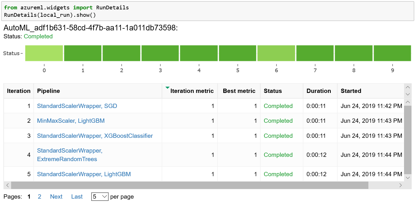
Figure 7-6. Automated ML widget UX
You can click any of the machine learning pipelines to explore more. In addition to a bunch of charts, you will see a feature importance chart. Use the legend to see overall model-level as well as class-level feature importance. In Figure 7-7, you can see that “petal width (cm)” is the most important feature from the overall model perspective, but “sepal width (cm)” is the most important feature for class 1.
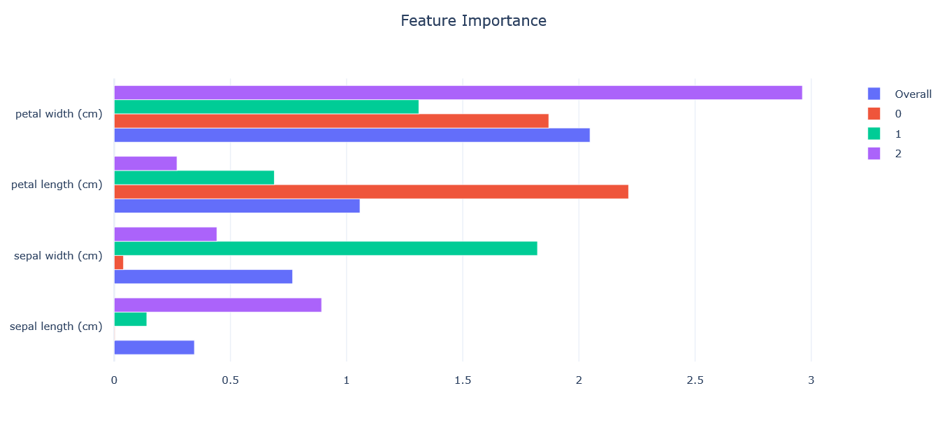
Figure 7-7. Feature importance in the automated ML widget UX
Model Transparency
In the previous section, you learned how feature importance is a powerful way to understand machine learning models. It is also important to understand the training process, from input data leading to the machine learning model. In this section, we will discuss how automated ML makes the end-to-end training process transparent.
Understanding the Automated ML Model Pipelines
As discussed in earlier chapters, automated ML recommends model pipelines with the goal of producing high-quality ML models based on user inputs. Each model pipeline includes the following steps:
-
Data preprocessing and feature engineering
-
Model training based on selected algorithm and hyperparameter values
With automated ML, you can analyze steps of each recommended pipeline before using them in your application or scenario. This transparency not only allows you to trust the model better, but also enables you to customize it further. For details on how to get visibility into the end-to-end process, refer to Chapter 4, which covers all of the steps in automated ML–recommended machine learning pipelines.
Guardrails
In previous chapters, you saw that automated ML makes it easy to get started with machine learning by automating most of the iterative and time-consuming steps. In addition, there are many best practices that you need to apply to achieve reliable results. Guardrails help users understand potential issues with their data and training model, so they know what to expect and can correct the issues for improved results.
Following are some common issues to be aware of:
- Missing values
-
As we’ve discussed in earlier chapters, real-world data isn’t clean and could be missing a lot of values. Before using it for machine learning, data with missing values needs to be “fixed.” Various techniques can be used to fix missing values, from dropping entire rows to using various techniques to intelligently populate missing values based on the rest of the data; this is called imputation.
- Class imbalance
-
Class imbalance is a major problem in machine learning because most machine learning algorithms assume that data is equally distributed. In the case of imbalanced data, majority classes dominate over minority classes, causing the machine learning models to be more biased toward majority classes. This results in poor classification of minority classes. Some real-world examples involve anomaly detection, fraud detection, and disease detection.
Sampling is a commonly used strategy to overcome class imbalance. There are two ways to sample:
- Data leakage
-
Data leakage is another key problem when building machine learning models. This occurs when the training dataset includes information that would not be available at the time of prediction. Because the actual outcome is already known (due to leakage), the model performance will be almost perfect for the training data but will be very bad during prediction. There are a few tricks you can use to overcome data leakage:
- Add noise
-
Add noise to input data to smooth out the effects of possibly leaky features.
As you can see, understanding and safeguarding against common issues like these can be critical to the performance of the model as well as transparency to users. Automated ML offers guardrails to show and protect against common issues and will continue to add more sophisticated ones over time.
Conclusion
In this chapter, we discussed two key aspects that become very important when establishing trust in a trained machine learning model: interpretability and transparency. Almost every company or team using machine learning models requires the models to be interpretable and transparent–to a degree–to gain confidence.
You learned how to take advantage of interpretability/explainability features by using the Azure Machine Learning Python SDK, as well as the automated ML Python SDK and widget UX. We also touched upon gaining visibility into end-to-end model-training pipelines as well as pitfalls to avoid, and why setting up guardrails against these pitfalls is important to ensure the transparency of your model.