Chapter 4
A pore-scale investigation of the dynamic response of saturated porous media to transient stresses
Christian Huber and Yanqing Su
School of Earth and Atmospheric Sciences, Georgia Institute of Technology, Atlanta, GA, USA
Abstract
The dynamical response of saturated porous media to transient stresses is complex because of the coupling between the solid and fluid phases. Over the last three decades, theoretical models have emerged and they predict that the transient response of porous media to pore-pressure fluctuations depends only on a single dimensionless number. This single parameter represents the ratio of the forcing frequency to a characteristic frequency of the medium. Although theoretical models for the frequency dependence of the effective permeability of the medium have successfully predicted the response of porous media at high frequency observed in laboratory and numerical experiments, they rely on assumptions that limit their applicability to homogeneous media and narrow pore-size distributions. We use pore-scale flow simulations with four different porous media topologies to study the effect of pore geometry and pore-size distribution on the dynamic response to transient pore-pressure forcing. We find a good agreement with published theoretical work for all but one medium that exhibits the broadest pore-size distribution and, therefore, the largest degree of pore-scale heterogeneity. Our results suggest the presence of a resonance peak at high frequency where the discharge, and therefore the effective permeability, is significantly amplified compared with their value around the resonant frequency. We suggest two interpretations to explain resonance. At the continuum scale, a finite speed of pore-pressure propagation during transients requires the addition of a correction term to Darcy's law. We derive a hyperbolic mass conservation equation that admits resonance under certain conditions. This model can explain the peak observed for one medium but fails to explain the absence of resonance displayed by the three other media. The second interpretation, motivated by the different pore-size distributions for the texture where resonance is observed, calls for pore-scale processes and heterogeneous pore-pressure distribution among primary and secondary flow pathways.
Key words: dynamic permeability, pore-scale modeling, saturated porous media
Introduction
The Earth's crust is porous and heterogeneous over a wide range of length scales (Ingebritsen & Manning 2010). In the upper few kilometers, the pore space is generally saturated with aqueous fluids that play a significant role in water–rock chemical reactions. Pore fluids also affect the physical properties of the heterogeneous medium. One of the most important properties for mass and heat transport is the permeability of the matrix to the flow of fluids. Besides long-term changes in permeability associated with chemical reactions and pore clogging, the response to rapid stress transients (dynamic stresses) can also significantly affect the effective permeability of saturated porous media because of poroelastic effects (Terzaghi 1925; Biot 1956a,b, 1962).
Maurice Biot developed the first theoretical model of the propagation of acoustic waves in saturated porous media in the mid-1950s. Biot found two independent solutions to the propagation of acoustic waves in porous media that he referred to as waves of the first and second kind. For both types of waves, the net drag force exerted by the solid matrix on the fluid controls the dissipation of mechanical energy and by extension the attenuation of the propagating waves. At low frequency, the wave of the second kind, sometimes referred to as Biot's slow wave, consists of pressure transport by diffusion (Darcy transport) and can lead to larger attenuation over the seismic frequency band (Pride et al. 2002). An important concept that emerged from the work of Biot is that the drag force that couples the fluid to the solid matrix is frequency dependent and can be represented as a dynamic correction on the effective fluid viscosity.
Following the seminal work of Biot, several groups studied the discharge of pore fluids subjected to harmonic pressure forcing and found, in agreement with Biot's analysis, the effective permeability of the medium to be frequency dependent and complex valued at high frequency (π/2 phase lag between the forcing and the discharge) (Biot 1962; Johnson et al. 1987; Smeulders et al. 1992; Berryman 2003). The frequency-dependent permeability is often referred to as the dynamic permeability of a medium. The Johnson–Koplik–Dashen (JKD) dynamic permeability model offered the first scaling relationship to model the frequency dependence of permeability (Johnson et al. 1987). It relies on a single tree parameter, the rollover frequency ωc, which depends on fluid and matrix properties. This critical frequency represents the transition from viscous- to inertia-dominated momentum balance in a homogeneous porous medium (order of kilohertz or higher for water-saturated sandstones) (Pride et al. 2002). Later, the model was verified experimentally and numerically using simple geometries (Johnson et al. 1987; Sheng & Zhou 1988; Smeulders et al. 1992; Muller & Sahay 20ll; Pazdniakou & Adler 2013). In addition, Smeulders et al. (1992) provided a more rigorous mathematical validation of the model using standard homogenization methods.
For the most part, pore-scale calculations have been limited to simple and highly symmetric geometries because of computational limitations. Numerical results showed a good agreement with the existence of a single scaling function (related to the critical frequency) that was assumed in Johnson et al. (1987). Recently, a pore-scale study using a lattice Boltzmann flow solver was able to extend the range of validation to more realistic geometries (Pazdniakou & Adler 2013). Their study actually solved for the dynamic permeability with a different problem setup. The porous medium is periodic and therefore infinite (no boundary conditions), the flow is buoyancy driven, and the forcing is homogeneous and applied through a transient harmonic perturbation of the bulk force responsible for the flow. In this study, we use a lattice Boltzmann pore-scale flow model to investigate different porous media topologies and their effect on the dynamic permeability and verify the scaling of the JKD model. Each domain has finite dimensions and the flow is pressure driven. The dynamic forcing is introduced by an imposed pore-pressure oscillation at one of the boundary. Although the difference in these two models is subtle, the choice of setup can lead to significantly different outcomes, and the effect of finite domains and pressure boundary conditions needs to be studied. We observe that the dynamic permeability response is generally in good agreement with the scaling proposed by Johnson et al. (1987) and Smeulders et al. (1992). We discuss these results in analogy to well-known properties of electric circuit involving a resistor and a capacitor in parallel (Debye relaxation).
In specific cases, however, we observe a significant departure from the JKD (or Debye relaxation) model. In particular, we observe features that suggest a resonance behavior that is not consistent with the theory of Johnson et al. (1987) and Smeulders et al. (1992). We propose two alternative explanations for the existence of resonance. First, using a continuum-scale argument, we discuss the importance of a correction term to Darcy's law for transient flows that allows us to derive a hyperbolic version of the mass conservation equation. We show that this new mass conservation equation converges to the standard parabolic diffusion of pore pressure at low frequency, but allows the propagation of damped waves and resonance at high frequency. Although this continuum-scale model offers a satisfying framework to explain the occurrence of resonance in one medium, it fails to explain the lack of resonance in the three other media. Alternatively, we suggest that pore-scale effects, such as different pore-size distributions (PSDs), can facilitate pore-pressure excitation between heterogeneous flow pathways in response to forced pore-pressure excitations.
Background
Maurice Biot (1962) introduced a model for the propagation of acoustic waves in saturated porous media by computing the net drag force between the fluid and an oscillating matrix under simplified geometry such as Poiseuille and duct flows. He showed that the drag associated with harmonic forcing leads to an effective fluid viscosity that can become complex and that displays a frequency dependence. It is important to note that Biot's approach was conducted at the pore scale and used an unsteady version of Stokes equation for the flow in the limit of a compressible fluid. The momentum equation represented, therefore, a balance between three terms: inertia, pressure, and viscous stresses.
Johnson et al. (1987) and Smeulders et al. (1992) showed that by matching inertial forces associated with the transient forcing with viscous forces, a critical frequency emerges

where η is the dynamic viscosity of the pore fluid, ρf its density, k0 the static permeability, φ the porosity of the medium, and lastly, α∞ is the dynamic tortuosity at infinite frequency of the medium, which is related to the formation factor F = φ/α∞ (Johnson et al. 1987).
The ratio of the forcing frequency ω to ωc controls the dynamic response of saturated (homogeneous) porous media to transient pore-pressure forcing. It is important to note that, in isotropic homogeneous media, the effect of the microstructure of the porous medium only emerges through three independent scalar parameters: the static (ω → 0) permeability, porosity, and formation factor of the medium. As discussed by Pride et al. (2002), once corrected for the dynamic permeability response, using mass conservation, the partial differential equation that describes the evolution of the pore pressure is a diffusion equation and is therefore parabolic and dissipative. We therefore expect that the forced pressure oscillations decay with time as expected from a diffusion equation.
Methods
Computation of the formation factor
We constructed four porous media synthetically either using a stochastic algorithm of crystal nucleation and growth following the method described in Hersum and Marsh (2006) (textures referred to as cuboids and spheres) or creating void space with simple geometrical shapes (e.g., spheres, tubes, and wavelike tubes). Figure 4.1 shows the pore structure of the four media.
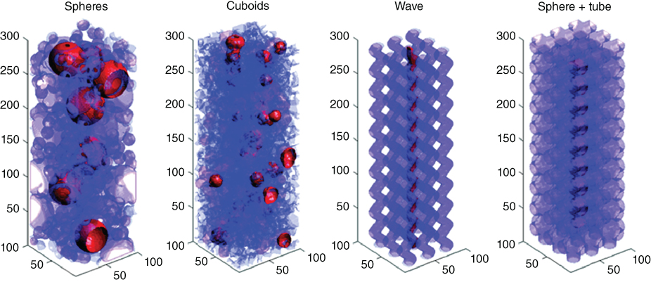
Fig. 4.1 Pore-scale representations of the four porous media. Warm colors (red) show larger pores. All textures are synthetically constructed; spheres and cuboids are constructed with a stochastic nucleation and growth algorithm following the procedure described in Hersum and Marsh (2006). (See color plate section for the color representation of this figure.)
The formation factor of a heterogeneous medium is defined as the effective electric conductivity of the medium normalized to that of the pore-filling fluid assuming the solid matrix is a perfect insulator. We use the analogy between the steady-state solution of the (heat) diffusion equation and the solution to Poisson's equation for the electric potential in heterogeneous media.
We apply a 3D lattice Boltzmann model for heat conduction in porous media. In the lattice Boltzmann method, the diffusion equation is modeled following a statistical approach, and it is replaced by a discrete version of Boltzmann's equation. Boltzmann's equation describes the evolution of particle probability functions g(x,v,t) that represent the probability of finding a particle at position x, traveling with velocity v at time t. Particles stream through the domain and collide with each other, which leads to the following equation for the evolution of the gis:
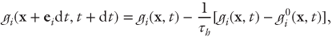
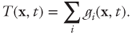
where it is assumed that the collision operator reduces to a single relaxation time (Bhatnagar et al. 1954). The index i refers the discrete set of possible trajectories ei on the lattice (nearest neighbors), τh is the relaxation time (related to the thermal diffusivity), and gi0 is the local equilibrium particle probability distribution function. The macroscopic field of interest, here temperature T(x,t), is obtained by summing the local distribution functions
The equilibrium distributions are linearly dependent on the local temperature
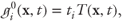
where ti is lattice weights, which in our model with seven discrete velocity ei are t0 = 1/4, t1–6 = 1/8 (see Fig. 4.2).
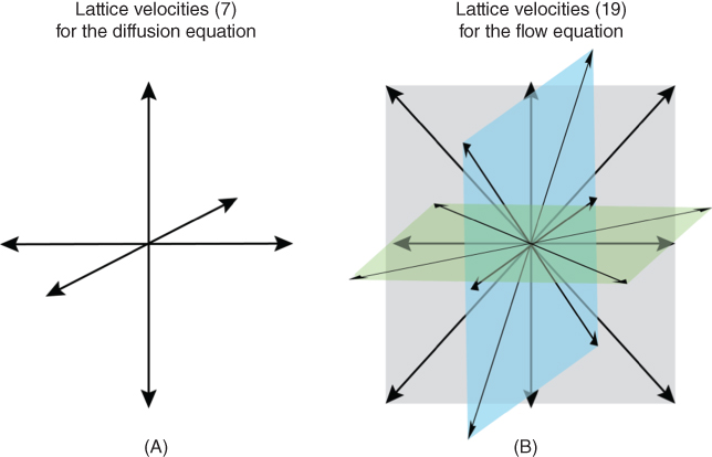
Fig. 4.2 Diagram showing the velocity discretization used for the lattice Boltzmann modeling. (A) The seven-velocity ei (including a rest velocity e0) model for the calculation of the formation factor is shown. (B) The 19-velocity model c, used for the flow calculations at the pore scale, is illustrated. (See color plate section for the color representation of this figure.)
This method has been shown to recover the diffusion equation in 3D and allows for a simple treatment of the internal solid–fluid boundaries (no heat flux). This is done with the bounce-back rule that specifies that distributions are reflected on solid obstacles
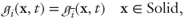
where the overbar denotes the velocity direction opposite to i; in other words, the distributions are all reflected backward when they encounter a solid node in the physical domain (Huber et al. 2008, 2010). In these calculations, the temperature at the inlet (z = 0) and outlet (z = Lz) is fixed to 1 and 0, respectively. The calculations are run until a steady state is reached. For more information about lattice Boltzmann models for the diffusion equation, the reader is referred to Wolf-Gladrow (2000).
Lattice Boltzmann model for fluid flow
Our pore-scale flow simulations are also based on the lattice Boltzmann method. We use the Palabos open-source library (www.palabos.org), to compute the 3D flow field at the pore scale in each medium. Similar to the calculations of the formation factor discussed earlier, we compute the evolution of particle probability density functions f(x,v,t) subjected to streaming (free flow) and collisions with other particles or boundaries where mass and momentum are conserved locally. The discretized form of the evolution equation for f(x,v,t) is similar as well
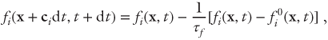
where τf is the relaxation time to the local equilibrium distribution functions fi0 and i is an index that discretizes the space of available trajectories for particles. Because of the four scalar fields that are conserved locally (one for mass and three for momentum), the particle motion is now limited to 19 directions; see Figure 4.2. After assigning the first statistical moments of the particle probability distribution functions fi to conserved macroscopic quantities such as local density and momentum
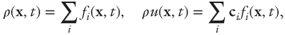
a multiscale expansion yields a compressible version of Navier–Stokes equations (Frisch et al. 1986, 1987; Higuera & Jimenez 1989). In the expansion, the kinematic viscosity of the fluid v is identified with
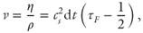
where  is a constant that depends on the choice of spatial discretization (1/3 here). In each calculation, pressure boundary conditions are applied at z = 0 and z = Lz. In the first stage, steady boundary conditions are applied to obtain a steady discharge through the medium. It allows us to calculate the static permeability

where Δp0 is the steady pressure drop imposed on the medium and the discharge is computed with
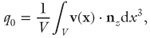
where v(x) is the steady-state pore-scale velocity field and nz the direction along the pressure gradient. After reaching a steady discharge, the outlet pressure is varied harmonically around its static value 

We compute the flow field and therefore calculate the discharge with a high temporal resolution during many pressure cycles to calculate the dynamic permeability. The amplitudes of the pressure fluctuations and gradients are small enough that the compressibility effect remains limited in our lattice Boltzmann simulations.
Postprocessing of transient discharge data
In response to the dynamic pore-pressure condition, the flux qout becomes
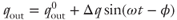
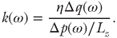
when the system reaches a quasi-steady state. φ is the phase lag between the flux and the imposed pressure oscillations. We fit the outlet discharge with a sine function A sin(ωt + B) + C to obtain the amplitude Δq and the phase φ. The dynamic permeability k(ω) is calculated as
By conducting simulations over a wide range of frequency, we can establish the spectral response of each medium to the pressure oscillations.
Results
Expected dynamical response
We selected four porous media structures to provide a test to the predicted self-similar nature of the dynamic response of the permeability in terms of frequency (Johnson et al. 1987; Smeulders et al. 1992). These textures range from about 30% to 60% porosity, the formation factors vary by a factor of 3, and the static permeability varies by a factor of 6. It is interesting to note that the JKD model for the dynamic permeability only depends on these three factors. We are also interested, within the limits of the number of porous media structures tested here, to investigate whether the PSD can affect the dynamical response independently from these three parameters.
The PSD for each medium is computed with the model of Yang et al. (2009), where in each pore, the largest sphere that can be fully included into the volume of the pore defines its effective radius (pore size). The results of these PSD calculations are shown in Figure 4.3. We note that the range of pore sizes for cuboids, sphere tubes, and waves are comparable but that spheres display a significantly greater range of pore sizes with several pores with radius >20 grid units.
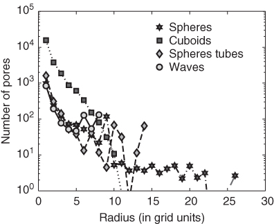
Fig. 4.3 Pore-size distribution for the four media calculated from the model of Yang et al. (2009). In this model, the radius of each pore is determined by the largest sphere that can be fully included into the pore.
The formation factors are computed according to the section Computation of the formation factor, where a 3D diffusion model is relaxed to steady state. An example of steady-state temperature distribution in the cuboids texture is shown in Figure 4.4 for reference, and the results are listed in Table 4.1.
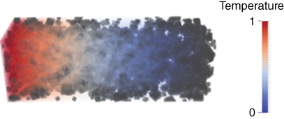
Fig. 4.4 Thermal field in the porous medium (cuboids) at steady state. Here, the solid fraction is assumed as a perfect insulator. The formation factor is computed from the effective thermal conductivity of the medium at steady state. (See color plate section for the color representation of this figure.)
Table 4.1 Summary of the steady flow calculations
| Name | Porosity φ | Formation factor F | Permeability k0 (dimensionless) | JKD critical frequency ωc |
| Spheres + tubes | 0.49 | 0.3 | 2.98 | 6.2 × 10⁴ |
| Waves | 0.21 | 0.11 | 0.48 | 1.4 × 10³ |
| Spheres | 0.61 | 0.15 | 0.89 | 1.05 × 10³ |
| Cuboids | 0.61 | 0.39 | 1.16 | 2.04 × 10³ |
For each porous medium, we conducted between 15 and 20 simulations with different forcing frequencies to obtain the effective permeability of the medium over a range of frequency that extends over 3 orders of magnitude.
In Figure 4.5A, we show the un-normalized results for three of the four media. We can clearly observe similar trends with a sudden decay of effective permeability as the forcing frequency approaches the critical frequency of each medium ωc (see vertical lines). Once the frequency is normalized with ωc (Fig. 4.5B), the data collapse as expected for the self-similar trend observed and documented by several authors (Johnson et al. 1987; Sheng & Zhou 1988; Smeulders et al. 1992; Müller & Sahay 2011; Pazdniakou & Adler 2013). We find an excellent agreement with the theory developed by Johnson et al. (1987) and Smeulders et al. (1992) irrespective of the PSD of the medium. The complex nature of the dynamic permeability is better portrayed by the phase lag between the harmonic pressure forcing and the computed discharge (Fig. 4.6) and again shows an excellent agreement with previous studies (Johnson et al. 1987; Sheng & Zhou 1988; Smeulders et al. 1992; Müller & Sahay 2011; Pazdniakou & Adler 2013).
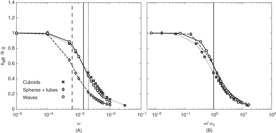
Fig. 4.5 Effective (dynamic) permeability as function of frequency for three of the four porous media used in this study. (A) How differences in porosity, static permeability k0, and formation factor influence the response. (B) The rollover frequency ωc provides a satisfying normalization factor to observe a self-similar behavior between the different media.
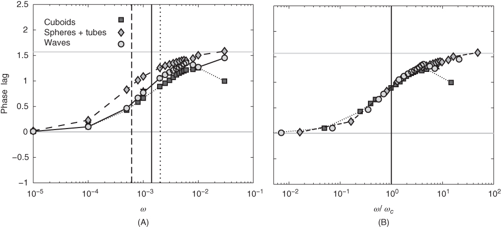
Fig. 4.6 The phase lag φ between the pore-pressure forcing at the outlet and the discharge in the porous medium as function of frequency (A) and normalized frequency (B). The results are consistent with previous studies (Johnson et al. 1987; Sheng & Zhou 1988; Smeulders et al. 1992; Müller & Sahay 2011; Pazdniakou & Adler 2013).
Anomalous behavior
We conducted the same simulations on the last porous medium (spheres) and obtained a significantly different result.
The work remains preliminary; however, the runs were checked for reproducibility and the results are robust. The dynamic response of the permeability and phase lag with the harmonic forcing is similar to what we observe for the other media except for the existence of a peak at high frequency ω > ωc (see Figs 4.7 and 4.8). The phase lag displays an excursion to negative phases (or in that context, positive phase with φ > π to satisfy causality) that coincides with the resonant permeability peak. We observed, although not shown here, a similar behavior in another medium that displayed sharp heterogeneities at the pore scale.
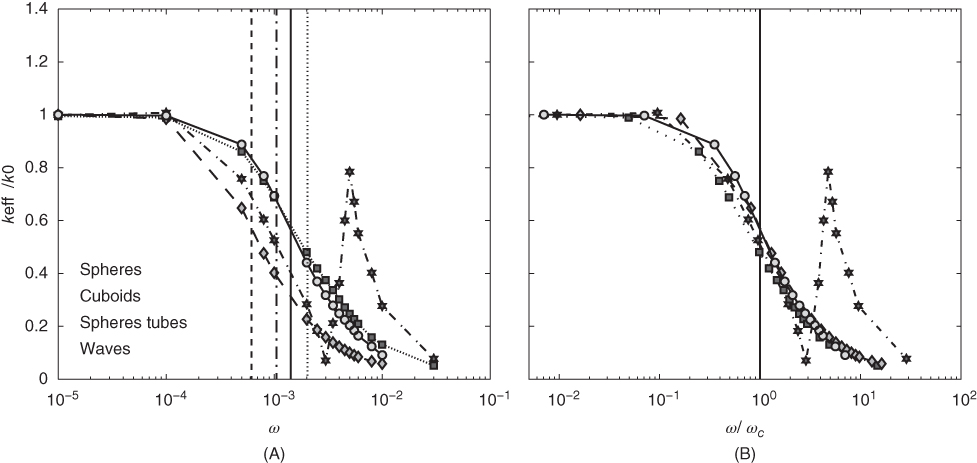
Fig. 4.7 Same as Figure 4.5 but with the last porous medium (spheres). Note that the medium referred to as spheres has the broadest pore-size distribution.
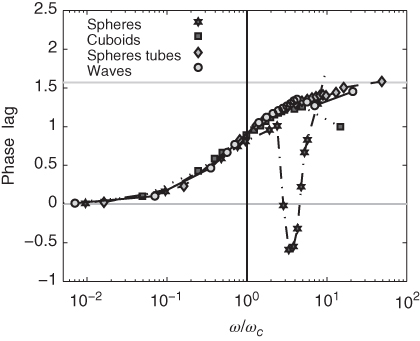
Fig. 4.8 Phase lag between the pore-pressure fluctuations and the discharge as function of normalized frequency for all media.
The existence of a permeability peak at high frequency is unexpected from the existing theory and suggests a resonance-like behavior over a narrow range of forcing frequencies. It is important to realize that neither Darcy's equation, even corrected for frequency-dependent permeability, nor the groundwater flow equation (diffusion) can cause a resonance-like behavior. Resonance occurs generally as a response to transient forcing of hyperbolic partial differential equations. In the Discussion section, we present an analogy between the standard JKD theory for the dynamic permeability and electric circuits and show that this theory fails to explain the peak observed in Figure 4.7. We discuss two possible causes for the peak in dynamic permeability: the resonance is governed by the dynamics at the continuum scale (modified Darcy flux) or by microstructural properties.
Discussion
Analogy to Debye relaxation
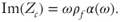
The linear theory of flow in porous media is often compared with linear electric circuit theory because of the many analogies between the two fields. First, Ohm's law is equivalent to Darcy's law with the hydraulic conductivity replacing the electrical conductivity and the head potential (or pseudopotential) as defined by Hubbert (1940) replacing the electrical potential. It is therefore natural to yield analogies between the dynamic permeability model presented by Johnson et al. (1987) and complemented by Smeulders et al. (1992) and the spectral response of electric circuits. The two equations that define the dynamic permeability and the dynamic tortuosity in the JKD model, once written in the frequency domain, are reminiscent to Ohm's law and the dynamical response of a capacitor, respectively
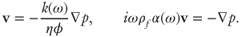
The second equation highlights the importance of inertia and shows that a phase lag exists at high frequency between the discharge φv and the pressure forcing. The π/2 phase between the current and the potential introduced by inertia is reminiscent of the effect of adding a capacitor to an electric circuit. If a resistor is set in parallel with a capacitor (see Fig. 4.9), the relative importance of the resistor and capacitor on the impedance of the circuit will be controlled by the imposed frequency and a Debye relaxation similar to the dynamical response of the permeability is obtained.
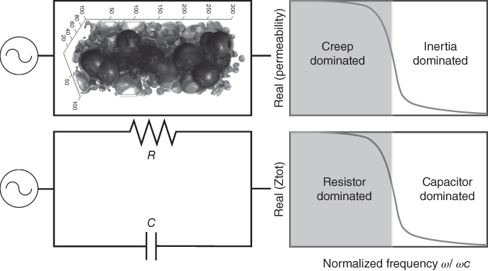
Fig. 4.9 Analogy between the dynamic permeability model of Johnson et al. (1987) and RC electric circuits in parallel. The spectral response of the effective permeability is similar to the spectral response of the overall impedance of the electric circuit.
The transition from creep- to inertia-dominated momentum dissipation in porous media is therefore similar to the response of a parallel RC circuit. We can even push the analogy further and use it to estimate the frequency at which we expect the transition to occur. The Debye frequency is obtained by matching the imaginary part of the capacitor impedance to that of the resistor

and hence, ωD = 1/RC. By analogy, the resistance in the dynamic version of Darcy's law is

while, using Eq. 4.14, the inertia associated with the capacitor can be defined as
Matching the two impedances allows us to retrieve the general form of the critical frequency of the JKD model

This analogy is useful because it also provides some clues as to what is problematic with the results that display resonance-like features.
Resonance and the importance of hyperbolic effects
One of the limitations of Darcy's law is that it represents a continuum approximation of a steady-state flow through a porous medium. The justification for using a time-independent momentum closure equation is that the Reynolds number that characterizes the flow is ≪1. Interestingly, regardless of this approximation, one can still derive a time-dependent mass conservation equation (a simple form of the groundwater flow equation) from Darcy's law that describes the pressure or head distribution in time and space in the porous medium
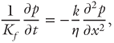
where for simplicity, the flow is assumed perpendicular to gravity, the permeability is homogeneous, and Kf refers to the fluid's bulk modulus. To be consistent with the theory developed by Johnson et al. (1987) and Smeulders et al. (1992), the solid matrix is viewed as incompressible for the sake of this argument. Equation 4.19 is a diffusion equation with the hydraulic diffusivity Dh = Kfk/η. The diffusion equation is parabolic, and consequently, the pore pressure can propagate at an infinite speed from the boundaries inside the domain. Consider an initial Dirac delta function of increased pore pressure centered at x = 0 at t = 0. At any t = dt, for any small dt, the pressure profile that results from Eq. 4.19 will have finite (nonzero) pressure values except at x → ±∞. The propagation of pressure is therefore instantaneous.
In reality, we know that it will take a finite time for pressure to propagate a finite distance in a porous medium. It is therefore necessary to introduce a transient term to modify Darcy's equation (even in the frequency domain, but we will restrict the analysis to the time domain here). A similar argument has been developed for heat transfer and the development of heat waves. Cattaneo (1958) and Vernotte (1958) arrived independently at the conclusion that a proper account of heat transfer by conduction should include an additional term in Fourier's law to consider that there is a finite time τ for the propagation of heat that depends on material properties. Following the same strategy, we arrive at the following definition for the transient Darcy's equation that satisfies a finite speed of pressure propagation
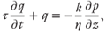
where q is the discharge in the z-direction. Although this equation is different from Biot's equations and the equations used by Johnson et al. (1987) and Smeulders et al. (1992), it is important to note some similarities. First, this equation is quite similar to the definition of unsteady Stokes flows and it is therefore not a novel concept. Also, in Biot's model, two separate but coupled equations were used to describe the displacement of each phase (fluid and solid) and Biot used an unsteady Stokes equation for the flow field that is not identical but quite similar to Eq. 4.20. The Cattaneo–Vernotte (CV) term in Eq. 4.20 (time derivative) introduces a phase lag for a finite value of τ, in agreement with the JKD model. The main difference here is that both Darcy's flux and the CV terms are balancing the pressure forcing in Eq. 4.19. The partitioning between the inertial term and the Darcian behavior depends on the value of the relaxation time τ and the forcing frequency ω; it is therefore not identical to Eq. 4.14.
Although the addition of a transient or unsteady term to the flux equation is not entirely novel, it is important to draw attention to its effect on the mass conservation equation. We argue that when Eq. 4.20 is introduced in the continuity equation, we retrieve a simple hyperbolic telegraph equation
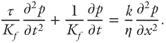
If the relaxation time τ ≪ 1, then the parabolic groundwater flow equation is retrieved. One can directly conclude that this hyperbolic equation admits the propagation of damped waves that travel with a finite velocity c = (KfF/ρf )1/2, where we identified the relaxation time τ with ρfk0/η = 1/ω. This means that our model is consistent with that of JKD where the transition between inertia- and viscous-dominated regimes occurs around the rollover frequency ωc. The adequate boundary conditions with respect to our study are
where Δp0 is the static pressure difference across the sample and Δp is the amplitude of the harmonic pressure perturbation. Using sine transforms
the mass conservation equation unfolds into n second-order nonhomogeneous ODE
The homogeneous equations that do not include the harmonic forcing yield solutions
where An and Bn are constants that are constrained by the initial and boundary conditions, and the characteristic frequencies ωn = n2π2kKf/ηLz2 and finally, γ = 1/τ. These solutions are dissipative (damping), and the damping increases when τ → 0, which is consistent with the diffusive behavior of the equation in this limit.
Because the harmonic forcing has no influence over the homogeneous solution, it is more important to study the particular solution for resonance effects. Because of the harmonic forcing, it is convenient to write the particular solutions as

The coefficients Cn and Dn are obtained after substituting Eq. 4.26 into Eq. 4.24
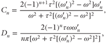
where the characteristic frequency of the medium  is defined by

The overall amplitude the waves associated with the particular solution in response to the forcing at frequency ω is
which implies a finite resonance when the forcing frequency ω approaches (but not equals)  . The actual solution for the resonant frequency requires finding the roots of a fifth-order polynomial (ω) that also depends on the choice of relaxation time τ and the order of the harmonic considered n. It is beyond the scope of this work to provide an analysis of this polynomial. It is, however, instructive to reflect on the amplitude of the particular solution as the forcing approaches resonance

which shows that the amplitude of high-frequency harmonics may become small. Only the lowermost modes may display visible resonance peaks. Moreover, in the limit where τ → 0, no resonance is observed, which is consistent with the character of the partial differential equation in that limit.
Our hyperbolic model for the mass conservation in a porous medium subjected to transient forcing therefore admits a resonant behavior if the relaxation time τ becomes important, that is, when ωτ > 1. Alternatively, resonance may occur when the forcing frequency approaches nπc/Lz, where c is the pressure wave propagation speed that depends on the compressibility of the fluid and the formation factor of the medium. There are obviously some simplifying assumptions in this model. For instance, we have assumed that τ was independent of frequency and we use the asymptotic limits for the permeability (k0) and the dynamic tortuosity to identify what governs the relaxation time using the standard equations for dynamic permeability. We therefore assume that τ is controlled by the physical properties of the porous medium and pore fluid and that it does not depend on the applied forcing. This assumption, although not justified, is consistent with the theory developed for heat wave propagation in heterogeneous media (Ozisik & Tzou 1994; Ordonez-Miranda & Alvarado-Gil 2011; Ordonez-Miranda et al. 2012).
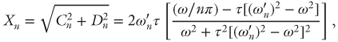
In light of this hyperbolic description of the mass balance in porous media, we can estimate the expected range of frequency that should display resonance for the different porous media. A satisfying model should be able to explain the peak observed with the spheres topology and be consistent with the absence of resonance observed for the three other media. We first compute  for n = 1 for all media. The actual resonance is not expected to take place exactly at
  , but from a visual inspection of the roots of the polynomial f(ω) the actual position of the resonance is
  . In Figure 4.10, we compare the set of forcing frequencies tested in our simulations with
  . The approximate range of frequency where the continuum hyperbolic mass balance equation predicts a resonant effect is consistent with our results with the spheres medium. However, we note that our calculations should have allowed us to observe a resonant peak in each medium. This informs us that while the continuum-scale hyperbolic model may be consistent for one of our medium at high frequency, the lack of resonance in the other media indicates that it is not sufficient to explain our results.
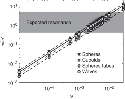
Fig. 4.10 Comparison between the sampled forcing frequency used in our simulations and the estimated range for the resonant frequency of the hyperbolic forced mass conservation equation ω*. We observe that our sampling should have allowed us to observe resonance in all four media. The dark grey ellipse marks the region where we observe resonance for the spheres data.
One could argue that the absence of resonance reflects that the amplitude of the particular solution is negligible and that the resonance is therefore difficult to measure. The hyperbolic model is generally consistent with the transient Stokes equation at the base of the theory of linear poroelasticity developed by Biot; however, it does not provide a satisfying explanation for our pore-scale simulations.
Alternatively, one can argue that pore-scale processes control the existence of the resonant peak. The porous media constructed by a stochastic process (spheres and cuboids) display more heterogeneity in terms of pore-scale structures. More specifically, the spheres medium was built with a broader PSD than the other three media. In heterogeneous media, at the pore scale, one should expect the plane wave assumption for the pressure propagation at the continuum scale to fail. In media that display competing pathways with different hydraulic responses, pore-pressure gradients can become significantly perpendicular to the main direction of propagation, and mass/pressure exchanges between different pathways may significantly affect the stress propagation. The visualization of the pore-pressure distribution in the spheres medium over time during one period can yield important information about the propagation of stress transients in the porous medium. Figure 4.11 shows snapshots of the pore-pressure field. We observe pressure waves propagating from the outlet (right) into the medium. An important feature worth noting is that at a fixed distance from the dynamic boundary (outlet), the pore pressure can vary significantly spatially. A possible explanation for the resonant behavior is that a heterogeneous porous medium can be viewed as a collection of connected primary and secondary pathways for the fluid and by extension pressure wave propagation. One clearly observes from Figure 4.11 that pressure fluctuations can propagate further into the medium along the main flow pathways creating some important pressure gradients perpendicular to the main flow direction. This should lead to significant mass exchanges between connected pathways with different transient responses to stress propagation.
Fig. 4.11 3D visualization of the pore-pressure field (normalized) at the forcing frequency corresponding to the maximum of the resonance peak in the spheres medium. The four images show the temporal evolution of the pressure field every quarter period. Note the regions with large lateral pore-pressure gradients (the imposed gradient is left to right) highlighted in red. It shows that flow pathways with different hydraulic connectivity have different response times to the forcing and that large pore-scale pore-pressure imbalance can emerge, violating the assumption of planar pressure wave propagating from the outlet. (See color plate section for the color representation of this figure.)
The resonant behavior may be associated with the existence of a finite time delay for the pore pressure to relax between primary and secondary pathways. If the response time for the pore-pressure exchange between competing but connected pathways approaches the period of the forcing, we argue that resonance may possibly occur. To test this hypothesis, we introduce a dimensionless variable ζ
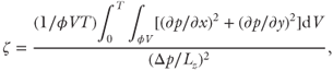
that quantifies the amount of transverse pressure gradient cumulated over a period T (2π/ω). If competing pathways with different characteristic response times coexist, we argue that transverse pressure gradients will become more important and ζ value increases. We computed ζ for all media at ω/ωc = 5, where the resonance peak maximum is found for the spheres medium. We find values of ζ = 0.9, 3.4, 40.1, and 130.1 for sphere tubes, waves, cuboids, and spheres, respectively. The medium exhibiting resonance is therefore characterized by a much greater ζ value than the other media, which suggests that transverse pore-scale pressure gradients are responsible for resonance.
Because these features in the spheres medium are sub-REV, it could explain the shortcomings of the continuum-scale interpretation to explain resonance. It is interesting to reflect on the major differences between our study and that of Pazdniakou and Adler (2013) where they do not observe resonance. Pazdniakou and Adler (2013) introduced the forcing as a homogenous oscillatory perturbation of a bulk force in the fluid and consider periodic and, therefore, infinite media. The homogeneous forcing applied in their study does not allow the buildup of significant pore-scale pressure gradients as the fluid responds uniformly to the perturbation instantaneously. There is no transport of the information on the changing pore pressure from the boundaries of the domain (there are no boundaries) and therefore no finite time response of the domain to the excitation. This could explain the different results between the two studies.
In the future, we plan on developing more highly heterogeneous structures at the pore scale and test whether resonance is promoted by pore-scale heterogeneities. In parallel, we suggest that an idealized theoretical model that decomposes the porous medium as a collection of regions according to the fluid's mobility may improve the continuum description of these heterogeneous media (dual- and multirate mass transfer models by Harvey & Gorelick 2000, Liu et al. 2007 and Porta et al. 2013). Such a framework including a finite relaxation time for pressure (leakage) between the more mobile and less mobile subsets of the medium could provide a framework to test whether pore-scale heterogeneity can influence a significant departure to the theory of JKD and even lead to resonant effects.
Conclusions
The propagation of pore-pressure transients in saturated porous media is complex at high frequency, when the short wavelength can interact with the heterogeneous structure of the medium. Over the last three decades, successful models for the dynamic response of porous media to harmonic pressure forcing have been developed and tested. They highlight that only three continuum-scale descriptors of the complex pore structure are important in homogeneous and isotropic media to characterize the spectral response of permeability. These descriptors are the porosity of the medium, its formation factor, and its static permeability. We have constructed four synthetic porous media from the pore scale with different porosity, formation factors, and permeability. Using a lattice Boltzmann method to compute the fluid flow at the pore scale, we find a very good agreement between our results and the theory for porous media with relatively narrow PSDs.
The medium that shows the broadest range of pore sizes, however, has a distinctive response to the imposed pressure transients. We observe a feature that resembles a resonance peak for the effective permeability at high frequency. Drawing from analogies with electric circuits and heat wave models, we postulate that the resonance feature is either governed by processes that operate at the continuum scale or by pore-scale processes that arise because of significant pore-scale heterogeneity. The development of a mass conservation equation at the continuum scale that corrects for the finite time required for pore pressure to propagate in the medium allows for resonance behavior to take place. It predicts resonance over the correct range of frequency for the case where our numerical results display resonant features. It, however, fails to explain the absence of resonance observed for the other media. Based on our numerical results, we argue that the resonance we observe is rather caused by pore-scale processes, whereby significant local pore-pressure gradients can form between heterogeneous flow pathways characterized by different response timescales to the imposed pressure excitations. Future studies focused on the distribution of pore pressure in heterogeneous media will potentially shed light on the dynamical processes that control the existence and the factors that govern the resonance of highly heterogeneous and saturated porous media.
Acknowledgments
C.H. and Y.S. thank Geofluids Editor C. Manning and acknowledge the thorough reviews of two anonymous reviewers and funding from an ACS-PRF DNI grant.