4.1 Introduction
Harmonic balance method [1] is one of the commonly used methods for analyzing the periodic solution of nonlinear systems. It transforms the problem of solving nonlinear differential equations into solving nonlinear algebraic equations, which greatly simplifies the analysis. However, the harmonic balance method has the following disadvantages: (1) It is only suitable for obtaining a steady-state solution but cannot be used for transient analysis; (2) If a periodic solution is approximated by harmonics containing orders from 0 (DC component) to N, then there will be (2N + 1) nonlinear algebraic equations to be solved. Hence, the amount of calculation using this method will increase sharply as N increases.
The general averaging method [2] proposed in [3] generalizes the harmonic balance method to transient analysis, and successfully analyzes the resonant converter and PWM (Pulse Width Modulation) switching converter. For a PWM switching converter with a duty cycle D close to 0 (or 1), it is not enough to estimate the waveform with only one harmonic. Therefore, it is often necessary to solve the higher harmonics. The general average method is not easy to solve higher harmonics. The reason is similar to the harmonic balance method, that is, if a solution needs to be approximated by harmonics containing orders from 0 (DC component) to N, then there will be (2N + 1) nonlinear algebraic equations to be solved. Thus, it is quite difficult to have the solutions, which usually need to be obtained numerically. For an open-loop PWM switching converter, although the problem is shown in the form of the linear differential equations, the number of orders is higher bringing about large amount of calculation. It is obvious that this method fails to overcome the second shortcoming of the harmonic balance method.
The equivalent-small-parameter method [4] introduces the perturbation technique into the harmonic balance method, and approximately converts the periodic solution into an expanded triangular series according to the (equivalent) small parameter. According to the order of the small parameters and the type of harmonics, the corresponding algebraic equations can be obtained. Hence, there is no need to solve nonlinear algebraic equations with many variables. In fact, the equivalent-small-parameter method is only applied to solve the nonlinear equations of the main oscillation. The other higher harmonics and corresponding correction terms can be obtained by solving the linear equations. The main oscillation only contains one or two harmonics, and the corresponding algebraic equation has fewer variables. It can be seen that the calculation amount is greatly reduced.
In this chapter, the equivalent-small-parameter method is used to analyze the PWM switching converters operating in CCM (continuous current mode) and DCM (discontinuous current mode), and the analytical expression of the steady-state periodic solution is obtained.
Furthermore, applying the idea in [2, 3], the equivalent-small-parameter method is generalized to the transient analysis of the PWM converter to obtain the equivalent differential (rather than algebraic) equations. Moreover, for open-loop PWM switching converters, only linear differential equations need to be solved. In [5], the progressive method is applied to the switching converter for analyzing transient process and ripple. However, the asymptotic method combines the transient and steady-state solutions, which results in complicated solution. The equivalent-small-parameter method clearly distinguishes the transient and steady-state solutions. Hence, the solution can be easily obtained.
4.2 General Method for Analysis of PWM Switching Power Converter by ESPM


 (k is an integer), which means the converter occupies (N + 1) sub-topologies during one switching cycle. The duty cycle of each sub-topology is defined as
  , and
, and  . The state variable vector
  is still expressed as the sum of the following main components and the order corrections:
 and
and  is the main component and the ith order correction term respectively. The parameter
  is introduced temporarily to indicate that different corrections would have different amplitudes, for example, the indicator
  means the
  is a small amount higher than
  , that is
  . Substituting (4.4) into (4.2) gives

 characterizes the periodic time-varying properties of the converter system. Correct processing of
  is the key to extend the equivalent small-parameter method to the analysis of switching converter systems. Since
  is a periodic function, it is usually expanded into a Fourier series, as follows.
![$$\delta^{(n)} = b_{0}^{(n)} + \sum\limits_{m = 1}^{\infty } {\left[ {b_{m}^{(n)} \exp (jm\tau ) + \bar{b}_{m}^{(n)} \exp ( - jm\tau )} \right]}$$](../images/419194_1_En_4_Chapter/419194_1_En_4_Chapter_TeX_Equ7.png)
![$$\begin{aligned} b_{0}^{(n)} & = d^{(n)} ,\quad b_{m}^{(n)} = \tfrac{1}{2}(\alpha_{m}^{(n)} - j\beta_{m}^{(n)} ),\quad m = 1,\,2\, \ldots \\ \alpha_{m}^{(n)} & = \left[ {\sin 2(\sum\limits_{k = 0}^{n} {d^{(k)} )m\pi } - \sin 2(\sum\limits_{k = 0}^{n - 1} {d^{(k)} )m\pi } } \right]/m\pi \\ \beta_{m}^{(n)} & = \left[ {\cos 2(\sum\limits_{k = 0}^{n - 1} {d^{(k)} )m\pi } - \cos 2(\sum\limits_{k = 0}^{n} {d^{(k)} )m\pi } } \right]/m\pi \\ \end{aligned}$$](../images/419194_1_En_4_Chapter/419194_1_En_4_Chapter_TeX_Equ8.png)

 decreases as m increases, it is generally assumed that
  contains a DC component and a fundamental component, and
  contains two adjacent higher harmonic components, namely:
 , the symbol
c.c represents the conjugate complex term (the meaning is the same below). Substituting (4.4) and (4.9) into (4.2) gives
, the symbol
c.c represents the conjugate complex term (the meaning is the same below). Substituting (4.4) and (4.9) into (4.2) gives
Using the same method as in Chap. 3, the main term  and the remainder
  of each nonlinear function vector
  are got according to Eq. (4.11), and then the steady-state periodic solution of the system is obtained according to Eq. (3.46).
4.3 Analysis of the Open-Loop Boost Converter Under CCM Operation
4.3.1 Modeling of the CCM-Boost Converter

CCM-Boost converter with its two equivalent topologies during one cycle
- (1)
The input power supply is ideal, that is, its internal resistance is ignored;
- (2)
Inductors and capacitors are considered as ideal components, that is, their parasitic parameters are not taken into account;
- (3)
Both the controllable switch ST and the diode SD are ideal switches, their on-resistance is zero, and the resistance is infinite when disconnected.
 (abbreviated as
  ) is defined to describe the on/off state of the switch ST, that is,
  when ST is on, and
  when ST is off. For the Boost converter operating in CCM, it is assumed that the controllable switch ST is turned on at the beginning of each switching cycle. After ton time, ST is turned off, and remains off state until the end of this cycle, then the definition of the switching function can be described by the following formula:
![$$\delta (t) = \left\{ {\begin{array}{ll} 1 & {t \in [nT,\,(n + d)T]} \\ 0 & {t \in [(n + d)T,\,(n + 1)T]} \\ \end{array} } \right.$$](../images/419194_1_En_4_Chapter/419194_1_En_4_Chapter_TeX_Equ12.png)

Nonlinear equivalent circuit of CCM-Boost converter
 and the capacitor voltage
  as the state variables, according to Fig. 4.2, the state differential equation describing the CCM-Boost converter can be obtained as follows:
![$${\mathbf{x}} = \left[ {\begin{array}{*{20}c} {i_{L} } & {v_{C} } \\ \end{array} } \right]^{Tr}$$](../images/419194_1_En_4_Chapter/419194_1_En_4_Chapter_TeX_IEq28.png) and p = d/dt, here the superscript “Tr” denote the transposition of a matrix, then the state differential equation of the above formula can be written in matrix form as follows
and p = d/dt, here the superscript “Tr” denote the transposition of a matrix, then the state differential equation of the above formula can be written in matrix form as follows
![$$G_{0} \left( p \right) = \left[ {\begin{array}{*{20}c} p & {\frac{1}{L}} \\ {\frac{ - 1}{C}} & {p + \frac{1}{RC}} \\ \end{array} } \right],\quad G_{1} \left( p \right) = \left[ {\begin{array}{*{20}c} 0 & {\frac{ - 1}{L}} \\ {\frac{1}{C}} & 0 \\ \end{array} } \right],\quad {\mathbf{u}} = \left[ {\begin{array}{*{20}c} {E/L} \\ 0 \\ \end{array} } \right]$$](../images/419194_1_En_4_Chapter/419194_1_En_4_Chapter_TeX_Equ15.png)

4.3.2 The Equivalent Mathematical Model Based on ESPM


Similarly, f0 and fi represent the main components and corrections of nonlinear vector function f(x) respectively.
 and
and  in Eq. (4.17) for state variables x can be expressed in the Fourier series as follows
 defined by (4.12) can be expanded into Fourier series as
![$$\delta = b_{0}^{{}} + \sum\limits_{m = 1}^{\infty } {\left[ {b_{m} \exp (jm\tau ) + \bar{b}_{m} \exp ( - jm\tau )} \right]}$$](../images/419194_1_En_4_Chapter/419194_1_En_4_Chapter_TeX_Equ22.png)

 contains only the DC component and the fundamental component, and
  contains the (2i)th and (2i + 1)th harmonic components, here
i = 1, 2, 3 …, is a positive integer, that is,
contains the (2i)th and (2i + 1)th harmonic components, here
i = 1, 2, 3 …, is a positive integer, that is,

 and
and  , and the residual
  is the same as described in Chap. 3. We can also refer to the specific solution process in the next section.
Each equation in (4.26) can be solved step by step by using the method of harmonic balance, where the first equation is used to obtain the main wave x0, and following equations are used to solve the corrections x1, x2, …, etc. If the harmonic amplitude in the kth correction xk is much smaller than those in the (k − 1)th correction xk−1, the calculation process is terminated. Hence, according to discussions above, the steady-state solution for the vector state variable Eq. (4.14) can be approximated by x ≈ x0 + x1 + x2 + …. Usually, as the low-pass filtering property of DC/DC converters, the magnitudes of harmonics with much higher frequencies are small, so they are neglected, and only the first three equations in Eq. (4.26) need to be solved, these solutions suffice for most technical applications.
4.3.3 The Steady-State Periodic Solution of the Boost Converter Based on ESPM
4.3.3.1 Solution of the Main Term
![$${\mathbf{x}}_{0} = {\mathbf{a}}_{00} = \left[ {\begin{array}{*{20}c} {I_{00} } & {V_{00} } \\ \end{array} } \right]^{Tr}$$](../images/419194_1_En_4_Chapter/419194_1_En_4_Chapter_TeX_Equ27.png)


![$$\left[ {{\mathbf{G}}_{0} (0) + {\mathbf{G}}_{1} (0)b_{0} } \right]{\mathbf{a}}_{00} = {\mathbf{u}}$$](../images/419194_1_En_4_Chapter/419194_1_En_4_Chapter_TeX_Equ30.png)
 and
and  can be obtained by setting the differential operator
p = 0 in Eq. (4.15). For the converter with open loop operation, the duty ratio d is a known amount, i.e. d = D, then Eq. (4.30) can be rewritten in the matrix form as
can be obtained by setting the differential operator
p = 0 in Eq. (4.15). For the converter with open loop operation, the duty ratio d is a known amount, i.e. d = D, then Eq. (4.30) can be rewritten in the matrix form as![$$\left( {\left[ {\begin{array}{*{20}c} 0 & {\frac{1}{L}} \\ { - \frac{1}{C}} & {\frac{1}{RC}} \\ \end{array} } \right] + \left[ {\begin{array}{*{20}c} 0 & { - \frac{D}{L}} \\ {\frac{D}{C}} & 0 \\ \end{array} } \right]} \right)\left[ {\begin{array}{*{20}c} {I_{00} } \\ {V_{00} } \\ \end{array} } \right] = \left[ {\begin{array}{*{20}c} {E/L} \\ 0 \\ \end{array} } \right]$$](../images/419194_1_En_4_Chapter/419194_1_En_4_Chapter_TeX_Equ31.png)

4.3.3.2 Solution of the First Correction Term

 means complex-conjugate, and a11 = [I11 V11]Tr. Substituting x0, x1, δ0 and δ1 into the equation
  , we can get

![$$[{\mathbf{G}}_{0} (j\omega ) + {\mathbf{G}}_{1} (j\omega )b_{0} ]{\mathbf{a}}_{11} = - {\mathbf{G}}_{1} (j\omega ) \cdot b_{1} {\mathbf{a}}_{00}$$](../images/419194_1_En_4_Chapter/419194_1_En_4_Chapter_TeX_Equ35.png)
 and
and  can be obtained by setting the differential operator
  in Eq. (4.15), as for the derivative of the exponential function, there is
pejkωt = (jkω)ejkωt (k is an integer, here k = 1). For the Boost converter under study, Eq. (4.35) can be rewritten in the matrix form as:
in Eq. (4.15), as for the derivative of the exponential function, there is
pejkωt = (jkω)ejkωt (k is an integer, here k = 1). For the Boost converter under study, Eq. (4.35) can be rewritten in the matrix form as:![$$\left( {\left[ {\begin{array}{*{20}c} {j\omega } & {\frac{1}{L}} \\ { - \frac{1}{C}} & {j\omega + \frac{1}{RC}} \\ \end{array} } \right] + \left[ {\begin{array}{*{20}c} 0 & { - \frac{D}{L}} \\ {\frac{D}{C}} & 0 \\ \end{array} } \right]} \right)\left[ {\begin{array}{*{20}c} {I_{11} } \\ {V_{11} } \\ \end{array} } \right] = \left[ {\begin{array}{*{20}c} 0 & {\frac{1}{L}} \\ {\frac{ - 1}{C}} & 0 \\ \end{array} } \right]\left[ {\begin{array}{*{20}c} {b_{1} I_{00} } \\ {b_{1} V_{00} } \\ \end{array} } \right]$$](../images/419194_1_En_4_Chapter/419194_1_En_4_Chapter_TeX_Equ36.png)
![$$\left\{ {\begin{array}{*{20}l} {I_{11} = \frac{{b_{1} V_{00} - (1 - D)V_{11} }}{j\omega L}} \hfill \\ {V_{11} = \frac{{b_{1} [(1 - D)V_{00} - j\omega LI_{00} ]}}{{(1 - D)^{2} + (j\omega )^{2} LC + j\omega L/R}}} \hfill \\ \end{array} } \right.$$](../images/419194_1_En_4_Chapter/419194_1_En_4_Chapter_TeX_Equ37.png)
4.3.3.3 Solution of the Second Correction Term

Here a20 = [I20 V20]Tr is the vector of dc values, it will give the corrections of dc components in a00, and a22 = [I22 V22]Tr and a23 = [I23 V23]Tr correspond to the amplitudes second- and third-harmonics of state variable x respectively.
 , we can get

![$$[G_{0} (0) + G_{1} (0)b_{0} ]{\mathbf{a}}_{20} = - G_{1} (0)(b_{1} {\bar{\mathbf{a}}}_{11} + \bar{b}_{1} {\mathbf{a}}_{11} )$$](../images/419194_1_En_4_Chapter/419194_1_En_4_Chapter_TeX_Equ40.png)
![$$[G_{0} (j2\omega ) + G_{1} (j2\omega )b_{0} ]{\mathbf{a}}_{22} = - G_{1} (j2\omega ) \cdot (b_{2} {\mathbf{a}}_{00} + b_{1} {\mathbf{a}}_{11} + b_{3} {\bar{\mathbf{a}}}_{11} )$$](../images/419194_1_En_4_Chapter/419194_1_En_4_Chapter_TeX_Equ41.png)
![$$[G_{0} (j3\omega ) + G_{1} (j3\omega )b_{0} ]{\mathbf{a}}_{23} = - G_{1} (j3\omega ) \cdot (b_{3} {\mathbf{a}}_{00} + b_{2} {\mathbf{a}}_{11} + b_{1} {\mathbf{a}}_{22} )$$](../images/419194_1_En_4_Chapter/419194_1_En_4_Chapter_TeX_Equ42.png)
Likewise, the coefficient matrix  and
and  can be obtained by setting the differential operator
  in Eq. (4.15), as for the derivative of the exponential function, there is
pejkωt = (jkω)ejkωt (here k = 0, 2, 3).
in Eq. (4.15), as for the derivative of the exponential function, there is
pejkωt = (jkω)ejkωt (here k = 0, 2, 3).
It should be noticed that during the derivation process, the term  in Eq. (4.40b) can be omitted with respect to the term
  , as the magnitudes of harmonics with higher frequencies are smaller than those with lower frequencies.
![$$\left( {\left[ {\begin{array}{*{20}c} 0 & {\frac{1}{L}} \\ { - \frac{1}{C}} & {\frac{1}{RC}} \\ \end{array} } \right] + \left[ {\begin{array}{*{20}c} 0 & { - \frac{D}{L}} \\ {\frac{D}{C}} & 0 \\ \end{array} } \right]} \right)\left[ {\begin{array}{*{20}c} {I_{20} } \\ {V_{20} } \\ \end{array} } \right] = \left[ {\begin{array}{*{20}c} 0 & {\frac{1}{L}} \\ {\frac{ - 1}{C}} & 0 \\ \end{array} } \right]\left[ {\begin{array}{*{20}c} {\bar{b}_{1} I_{11} + b_{1} \bar{I}_{11} } \\ {\bar{b}_{1} V_{11} + b_{1} \bar{V}_{11} } \\ \end{array} } \right]$$](../images/419194_1_En_4_Chapter/419194_1_En_4_Chapter_TeX_Equ43.png)

![$$\left( {\left[ {\begin{array}{*{20}c} {j2\omega } & {\frac{1}{L}} \\ { - \frac{1}{C}} & {j2\omega + \frac{1}{RC}} \\ \end{array} } \right] + \left[ {\begin{array}{*{20}c} 0 & { - \frac{D}{L}} \\ {\frac{D}{C}} & 0 \\ \end{array} } \right]} \right)\left[ {\begin{array}{*{20}c} {I_{22} } \\ {V_{22} } \\ \end{array} } \right] = \left[ {\begin{array}{*{20}c} 0 & {\frac{1}{L}} \\ {\frac{ - 1}{C}} & 0 \\ \end{array} } \right]\left[ {\begin{array}{*{20}c} {b_{1} I_{11} + b_{2} I_{00} + b_{3} \bar{I}_{11} } \\ {b_{1} V_{11} + b_{2} V_{00} + b_{3} \bar{V}_{11} } \\ \end{array} } \right]$$](../images/419194_1_En_4_Chapter/419194_1_En_4_Chapter_TeX_Equ45.png)
![$$\left( {\left[ {\begin{array}{*{20}c} {j3\omega } & {\frac{1}{L}} \\ { - \frac{1}{C}} & {j3\omega + \frac{1}{RC}} \\ \end{array} } \right] + \left[ {\begin{array}{*{20}c} 0 & { - \frac{D}{L}} \\ {\frac{D}{C}} & 0 \\ \end{array} } \right]} \right)\left[ {\begin{array}{*{20}c} {I_{23} } \\ {V_{23} } \\ \end{array} } \right] = \left[ {\begin{array}{*{20}c} 0 & {\frac{1}{L}} \\ {\frac{ - 1}{C}} & 0 \\ \end{array} } \right]\left[ {\begin{array}{*{20}c} {b_{1} I_{22} + b_{2} I_{11} + b_{3} I_{00} } \\ {b_{1} V_{22} + b_{2} V_{11} + b_{3} V_{00} } \\ \end{array} } \right]$$](../images/419194_1_En_4_Chapter/419194_1_En_4_Chapter_TeX_Equ46.png)


Values of aik for CCM-Boost converter
i | k | aik | |
|---|---|---|---|
Vik | Iik | ||
0 | 0 |
|
|
1 | 1 |
|
|
2 | 0 |
|
|
2 |
|
| |
3 |
|
| |


![$$\begin{aligned} {\mathbf{x}} & = \left[ {\begin{array}{*{20}c} {i_{L} } & {v_{C} } \\ \end{array} } \right]^{Tr} \\ & = \left( {{\mathbf{a}}_{00} + {\mathbf{a}}_{02} } \right) + \left( {{\mathbf{a}}_{11} e^{j\tau } + {\mathbf{a}}_{22} e^{j2\tau } + {\mathbf{a}}_{32} e^{j3\tau } + c.c} \right) \\ \end{aligned}$$](../images/419194_1_En_4_Chapter/419194_1_En_4_Chapter_TeX_Equ51.png)


4.3.4 Simulations
Circuit parameters of the open-loop Boost converter
Parameters | Values |
|---|---|
Input voltage E | 37.5 V |
Switching frequency f | 1 kHz |
Inductance L | 6 mH |
Capacitance C | 45 μF |
Load resistance R | 30 Ω |
Duty ratio D | 0.25 |
![$${\mathbf{x}} = \left[ {\begin{array}{*{20}c} {i_{L} } & {v_{C} } \\ \end{array} } \right]^{Tr}$$](../images/419194_1_En_4_Chapter/419194_1_En_4_Chapter_TeX_IEq62.png) can be obtained as follows, here
can be obtained as follows, here  is the inductor current and
  is the voltage over the output capacitor.
 , and Fig. 4.4 shows the comparison waveforms with
  . It can be seen that the results from the ESPM are in good coincidence with those from simulations, indicating that the ESPM can analyze the steady-state solution of the open-loop converter well. Even when the operating frequency of the converter is small, such as
  , the state variable ripple is relatively large, the ESPM can still effectively obtain the analytical expression of the periodic solution of the converter, and only three iterations are needed to obtain enough precision. It can be seen that the equivalent small-parameter method is effective for analyzing the strong nonlinear system of the switching converter.
Steady-state ripple waveforms of state variables for CCM-Boost converter with fs = 1 kHz

Steady-state ripple waveforms of state variables for CCM-Boost converter with fs = 10 kHz
4.4 Analysis of the Open-Loop Buck Converter Under CCM Operation
4.4.1 Modeling of the CCM-Buck Converter

CCM-Buck converter with its two equivalent topologies during one cycle

Nonlinear equivalent circuit of CCM-Buck converter
 and the capacitor voltage
  as the state variables, according to Fig. 4.6, the state differential equation describing the CCM-Buck converter can be obtained as follows:
![$${\mathbf{x}} = \left[ {\begin{array}{*{20}c} {i_{L} } & {v_{C} } \\ \end{array} } \right]^{Tr}$$](../images/419194_1_En_4_Chapter/419194_1_En_4_Chapter_TeX_IEq70.png) and p = d/dt, then the state differential equation of the above formula can be written in matrix form as follows
and p = d/dt, then the state differential equation of the above formula can be written in matrix form as follows

![$$G_{0} \left( p \right) = \left[ {\begin{array}{*{20}c} p & {\frac{1}{L}} \\ {\frac{ - 1}{C}} & {p + \frac{1}{RC}} \\ \end{array} } \right],\quad G_{1} \left( p \right) = \left[ {\begin{array}{*{20}c} 0 & {\frac{ - 1}{L}} \\ 0 & 0 \\ \end{array} } \right],\quad {\mathbf{e}} = \left[ {\begin{array}{*{20}c} 0 \\ E \\ \end{array} } \right]$$](../images/419194_1_En_4_Chapter/419194_1_En_4_Chapter_TeX_Equ58.png)
4.4.2 The Equivalent Mathematical Model Based on ESPM


4.4.3 The Steady-State Periodic Solution of the Buck Converter Based on ESPM
![$${\mathbf{x}}_{0} = {\mathbf{a}}_{00} = \left[ {\begin{array}{*{20}c} {I_{00} } & {V_{00} } \\ \end{array} } \right]^{Tr}$$](../images/419194_1_En_4_Chapter/419194_1_En_4_Chapter_TeX_Equ61.png)
 , and hence we can get

![$$\left[ {\begin{array}{*{20}c} 0 & {\frac{1}{L}} \\ { - \frac{1}{C}} & {\frac{1}{RC}} \\ \end{array} } \right]\left[ {\begin{array}{*{20}c} {I_{00} } \\ {V_{00} } \\ \end{array} } \right] = \left[ {\begin{array}{*{20}c} 0 & {\frac{{b_{0} }}{L}} \\ 0 & 0 \\ \end{array} } \right]\left[ {\begin{array}{*{20}c} 0 \\ E \\ \end{array} } \right]$$](../images/419194_1_En_4_Chapter/419194_1_En_4_Chapter_TeX_Equ64.png)


 , and the following expressions for f1m and R2 can be got as

![$$\left[ {\begin{array}{*{20}c} {j\omega } & {\frac{1}{L}} \\ { - \frac{1}{C}} & {j\omega + \frac{1}{RC}} \\ \end{array} } \right]\left[ {\begin{array}{*{20}c} {I_{11} } \\ {V_{11} } \\ \end{array} } \right] = \left[ {\begin{array}{*{20}c} 0 & {\frac{{b_{1} }}{L}} \\ 0 & 0 \\ \end{array} } \right]\left[ {\begin{array}{*{20}c} 0 \\ E \\ \end{array} } \right]$$](../images/419194_1_En_4_Chapter/419194_1_En_4_Chapter_TeX_Equ68.png)

 , there is
  , thus one can obtain the following two equations

![$$\left[ {\begin{array}{*{20}c} {j2\omega } & {\frac{1}{L}} \\ { - \frac{1}{C}} & {j2\omega + \frac{1}{RC}} \\ \end{array} } \right]\left[ {\begin{array}{*{20}c} {I_{22} } \\ {V_{22} } \\ \end{array} } \right] = \left[ {\begin{array}{*{20}c} 0 & {\frac{{b_{2} }}{L}} \\ 0 & 0 \\ \end{array} } \right]\left[ {\begin{array}{*{20}c} 0 \\ E \\ \end{array} } \right]$$](../images/419194_1_En_4_Chapter/419194_1_En_4_Chapter_TeX_Equ72.png)
![$$\left[ {\begin{array}{*{20}c} {j3\omega } & {\frac{1}{L}} \\ { - \frac{1}{C}} & {j3\omega + \frac{1}{RC}} \\ \end{array} } \right]\left[ {\begin{array}{*{20}c} {I_{23} } \\ {V_{23} } \\ \end{array} } \right] = \left[ {\begin{array}{*{20}c} 0 & {\frac{{b_{3} }}{L}} \\ 0 & 0 \\ \end{array} } \right]\left[ {\begin{array}{*{20}c} 0 \\ E \\ \end{array} } \right]$$](../images/419194_1_En_4_Chapter/419194_1_En_4_Chapter_TeX_Equ73.png)
Values of aik for CCM-Buck converter
i | k | aik | |
|---|---|---|---|
Vik | Iik | ||
0 | 0 |
|
|
1 | 1 |
|
|
2 |
|
| |
3 |
|
| |


And the coefficient bi are still determined by Eq. (4.48).
4.4.4 Simulations
The circuit parameters of the open-loop Buck converter is list in Table 4.5.
![$${\mathbf{x}} = \left[ {\begin{array}{*{20}c} {i_{L} } & {v_{C} } \\ \end{array} } \right]^{Tr}$$](../images/419194_1_En_4_Chapter/419194_1_En_4_Chapter_TeX_IEq83.png) can be obtained as follows, here
can be obtained as follows, here  is the inductor current and
  is the voltage over the output capacitor.
Circuit parameters of the open-loop Buck converter
Parameters | Values |
|---|---|
Input voltage E | 15 V |
Switching frequency f | 50 kHz |
Inductance L | 150 μH |
Capacitance C | 4.7 μF |
Load resistance R | 10 Ω |
Duty ratio D | 0.35 |

It should be noted that, as the amplitude of the 3rd harmonic is quite small, which is ignored in (4.69).

Steady-state ripple waveforms of state variables for CCM-Buck converter
4.5 Analysis of the Open-Loop Cuk Converter Under CCM Operation
4.5.1 Modeling of the CCM-Cuk Converter

CCM-Cuk converter with its two equivalent topologies during one cycle

Nonlinear equivalent circuit of CCM-Cuk converter
 ,
,  and the capacitor voltages
  ,
, as the state variables, according to Fig. 4.9, the state differential equation describing the CCM-Cuk
converter can be obtained as follows:
as the state variables, according to Fig. 4.9, the state differential equation describing the CCM-Cuk
converter can be obtained as follows:
![$${\mathbf{x}} = \left[ {\begin{array}{*{20}c} {i_{1} } & {i_{2} } & {v_{1} } & {v_{2} } \\ \end{array} } \right]^{Tr}$$](../images/419194_1_En_4_Chapter/419194_1_En_4_Chapter_TeX_IEq90.png) and p = d/dt, then the state differential equation of the above formula can be written in matrix form as follows
and p = d/dt, then the state differential equation of the above formula can be written in matrix form as follows

![$$G_{0} \left( p \right) = \left[ {\begin{array}{*{20}l} p \hfill & 0 \hfill & {\frac{1}{{L_{1} }}} \hfill & 0 \hfill \\ 0 \hfill & p \hfill & 0 \hfill & {\frac{1}{{L_{2} }}} \hfill \\ {\frac{ - 1}{{C_{1} }}} \hfill & 0 \hfill & p \hfill & 0 \hfill \\ 0 \hfill & {\frac{ - 1}{C}} \hfill & 0 \hfill & {p + \frac{1}{RC}} \hfill \\ \end{array} } \right],\quad G_{1} \left( p \right) = \left[ {\begin{array}{*{20}l} 0 \hfill & 0 \hfill & {\frac{ - 1}{{L_{1} }}} \hfill & 0 \hfill \\ 0 \hfill & 0 \hfill & {\frac{ - 1}{{L_{1} }}} \hfill & 0 \hfill \\ {\frac{1}{{C_{1} }}} \hfill & {\frac{1}{{C_{1} }}} \hfill & 0 \hfill & 0 \hfill \\ 0 \hfill & 0 \hfill & 0 \hfill & 0 \hfill \\ \end{array} } \right],\quad {\mathbf{u}} = \left[ {\begin{array}{*{20}c} {E/L_{1}} \\ \begin{aligned} 0 \hfill \\ 0 \hfill \\ 0 \hfill \\ \end{aligned} \\ \end{array} } \right]$$](../images/419194_1_En_4_Chapter/419194_1_En_4_Chapter_TeX_Equ78.png)
Equations (4.71) and (4.72) are identical in form to Eqs. (4.14) and (4.16) respectively. And the equivalent mathematical model of the CCM-operated Cuk converter is also the same as Eq. (4.26), which can be solved in exactly the same way as in Sect. 4.3.
4.5.2 The Steady-State Periodic Solution of the Cuk Converter Based on ESPM
![$${\mathbf{x}}_{0} = {\mathbf{a}}_{00} = \left[ {\begin{array}{*{20}c} {I_{100} } & {I_{200} } & {V_{100} } & {V_{200} } \\ \end{array} } \right]^{Tr}$$](../images/419194_1_En_4_Chapter/419194_1_En_4_Chapter_TeX_Equd.png)
![$$\left[ {{\mathbf{G}}_{0} (0) + {\mathbf{G}}_{1} (0)b_{0} } \right]{\mathbf{a}}_{00} = {\mathbf{u}}$$](../images/419194_1_En_4_Chapter/419194_1_En_4_Chapter_TeX_Equ79.png)
 and
and  can be obtained by setting the differential operator
p = 0 in Eq. (4.73). For the converter with open loop operation, the duty ratio d is a known amount, i.e. d = D, then Eq. (4.74) can be rewritten in the matrix form as
can be obtained by setting the differential operator
p = 0 in Eq. (4.73). For the converter with open loop operation, the duty ratio d is a known amount, i.e. d = D, then Eq. (4.74) can be rewritten in the matrix form as![$$\left( {\left[ {\begin{array}{*{20}l} 0 \hfill & 0 \hfill & {\tfrac{1}{{L_{1} }}} \hfill & 0 \hfill \\ 0 \hfill & 0 \hfill & 0 \hfill & {\tfrac{1}{{L_{2} }}} \hfill \\ {\tfrac{ - 1}{{C_{1} }}} \hfill & 0 \hfill & 0 \hfill & 0 \hfill \\ 0 \hfill & {\tfrac{ - 1}{C}} \hfill & 0 \hfill & {\tfrac{1}{RC}} \hfill \\ \end{array} } \right] + \left[ {\begin{array}{*{20}l} 0 \hfill & 0 \hfill & {\tfrac{ - D}{{L_{1} }}} \hfill & 0 \hfill \\ 0 \hfill & 0 \hfill & {\tfrac{ - D}{{L_{1} }}} \hfill & 0 \hfill \\ {\tfrac{D}{{C_{1} }}} \hfill & {\tfrac{D}{{C_{1} }}} \hfill & 0 \hfill & 0 \hfill \\ 0 \hfill & 0 \hfill & 0 \hfill & 0 \hfill \\ \end{array} } \right]} \right) \cdot \left[ {\begin{array}{*{20}c} {I_{100} } \\ {I_{200} } \\ {V_{100} } \\ {V_{200} } \\ \end{array} } \right] = \left[ {\begin{array}{*{20}c} {\tfrac{1}{{L_{1} }}E} \\ \begin{aligned} 0 \hfill \\ 0 \hfill \\ 0 \hfill \\ \end{aligned} \\ \end{array} } \right]$$](../images/419194_1_En_4_Chapter/419194_1_En_4_Chapter_TeX_Equ80.png)


 means complex-conjugate, and a11 = [I111 I211 V111 V211]Tr. And a11 can be got from the following equation as
![$$[{\mathbf{G}}_{0} (j\omega ) + {\mathbf{G}}_{1} (j\omega )b_{0} ]{\mathbf{a}}_{11} = - {\mathbf{G}}_{1} (j\omega ) \cdot b_{1} {\mathbf{a}}_{00}$$](../images/419194_1_En_4_Chapter/419194_1_En_4_Chapter_TeX_Equ81.png)
 and
and  can be obtained by setting the differential operator
  in Eq. (4.73). For the Cuk converter under study, Eq. (4.76) can be rewritten in the matrix form as:
![$$\left( {\left[ {\begin{array}{*{20}l} j\omega \hfill & 0 \hfill & {\tfrac{1}{{L_{1} }}} \hfill & 0 \hfill \\ 0 \hfill & j\omega \hfill & 0 \hfill & {\tfrac{1}{{L_{2} }}} \hfill \\ {\tfrac{ - 1}{{C_{1} }}} \hfill & 0 \hfill & j\omega \hfill & 0 \hfill \\ 0 \hfill & {\tfrac{ - 1}{C}} \hfill & 0 \hfill & {j\omega+\tfrac{1}{RC}} \hfill \\ \end{array} } \right] + \left[ {\begin{array}{*{20}l} 0 \hfill & 0 \hfill & {\tfrac{ - D}{{L_{1} }}} \hfill & 0 \hfill \\ 0 \hfill & 0 \hfill & {\tfrac{ - D}{{L_{1} }}} \hfill & 0 \hfill \\ {\tfrac{D}{{C_{1} }}} \hfill & {\tfrac{D}{{C_{1} }}} \hfill & 0 \hfill & 0 \hfill \\ 0 \hfill & 0 \hfill & 0 \hfill & 0 \hfill \\ \end{array} } \right]} \right) \cdot \left[ {\begin{array}{*{20}c} {I_{111} } \\ {I_{211} } \\ {V_{111} } \\ {V_{211} } \\ \end{array} } \right] = \left[ {\begin{array}{*{20}l} 0 \hfill & 0 \hfill & {\tfrac{ - 1}{{L_{1} }}} \hfill & 0 \hfill \\ 0 \hfill & 0 \hfill & {\tfrac{ - 1}{{L_{1} }}} \hfill & 0 \hfill \\ {\tfrac{1}{{C_{1} }}} \hfill & {\tfrac{1}{{C_{1} }}} \hfill & 0 \hfill & 0 \hfill \\ 0 \hfill & 0 \hfill & 0 \hfill & 0 \hfill \\ \end{array} } \right]\left[ {\begin{array}{*{20}c} {b_{1} I_{100} } \\ \begin{aligned} b_{1} I_{200} \hfill \\ b_{1} V_{100} \hfill \\ b_{1} V_{200} \hfill \\ \end{aligned} \\ \end{array} } \right]$$](../images/419194_1_En_4_Chapter/419194_1_En_4_Chapter_TeX_Equ82.png)

Here a20 = [I120 I220 V120 V220]Tr is the vector of DC values, it will give the corrections of DC components in a00, and a22 = [I122 I222 V122 V222]Tr and a23 = [I123 I223 V123 V223]Tr correspond to the amplitudes of second- and third-harmonics of state variable x respectively.
![$$[G_{0} (0) + G_{1} (0)b_{0} ]{\mathbf{a}}_{20} = - G_{1} (0)(b_{1} {\bar{\mathbf{a}}}_{11} + \bar{b}_{1} {\mathbf{a}}_{11} )$$](../images/419194_1_En_4_Chapter/419194_1_En_4_Chapter_TeX_Equ83.png)
![$$[G_{0} (j2\omega ) + G_{1} (j2\omega )b_{0} ]{\mathbf{a}}_{22} = - G_{1} (j2\omega ) \cdot (b_{2} {\mathbf{a}}_{00} + b_{1} {\mathbf{a}}_{11} + b_{3} {\bar{\mathbf{a}}}_{11} )$$](../images/419194_1_En_4_Chapter/419194_1_En_4_Chapter_TeX_Equ84.png)
![$$[G_{0} (j3\omega ) + G_{1} (j3\omega )b_{0} ]{\mathbf{a}}_{23} = - G_{1} (j3\omega ) \cdot (b_{3} {\mathbf{a}}_{00} + b_{2} {\mathbf{a}}_{11} + b_{1} {\mathbf{a}}_{22} )$$](../images/419194_1_En_4_Chapter/419194_1_En_4_Chapter_TeX_Equ85.png)
 and
and  can be obtained by setting the differential operator
  in Eq. (4.73) (here k = 0, 2, 3). Equation (4.78) can be rewritten in matrix form as:
![$$\left( {\left[ {\begin{array}{*{20}l} 0 \hfill & 0 \hfill & {\tfrac{1}{{L_{1} }}} \hfill & 0 \hfill \\ 0 \hfill & 0 \hfill & 0 \hfill & {\tfrac{1}{{L_{2} }}} \hfill \\ {\tfrac{ - 1}{{C_{1} }}} \hfill & 0 \hfill & 0 \hfill & 0 \hfill \\ 0 \hfill & {\tfrac{ - 1}{C}} \hfill & 0 \hfill & {\tfrac{1}{RC}} \hfill \\ \end{array} } \right] + \left[ {\begin{array}{*{20}l} 0 \hfill & 0 \hfill & {\tfrac{ - D}{{L_{1} }}} \hfill & 0 \hfill \\ 0 \hfill & 0 \hfill & {\tfrac{ - D}{{L_{1} }}} \hfill & 0 \hfill \\ {\tfrac{D}{{C_{1} }}} \hfill & {\tfrac{D}{{C_{1} }}} \hfill & 0 \hfill & 0 \hfill \\ 0 \hfill & 0 \hfill & 0 \hfill & 0 \hfill \\ \end{array} } \right]} \right)\left[ {\begin{array}{*{20}c} {I_{120} } \\ {I_{220} } \\ {V_{120} } \\ {V_{220} } \\ \end{array} } \right] = \left[ {\begin{array}{*{20}l} 0 \hfill & 0 \hfill & {\tfrac{ - 1}{{L_{1} }}} \hfill & 0 \hfill \\ 0 \hfill & 0 \hfill & {\tfrac{ - 1}{{L_{1} }}} \hfill & 0 \hfill \\ {\tfrac{1}{{C_{1} }}} \hfill & {\tfrac{1}{{C_{1} }}} \hfill & 0 \hfill & 0 \hfill \\ 0 \hfill & 0 \hfill & 0 \hfill & 0 \hfill \\ \end{array} } \right] \cdot \left[ {\begin{array}{*{20}l} {\bar{b}_{1} I_{111} + b_{1} \bar{I}_{111} } \hfill \\ {\bar{b}_{1} I_{211} + b_{1} \bar{I}_{211} } \hfill \\ {\bar{b}_{1} V_{111} + b_{1} \bar{V}_{111} } \hfill \\ {\bar{b}_{1} V_{211} + b_{1} \bar{V}_{211} } \hfill \\ \end{array} } \right]$$](../images/419194_1_En_4_Chapter/419194_1_En_4_Chapter_TeX_Equ86.png)
![$$\begin{aligned} & \left( {\left[ {\begin{array}{*{20}l} {j2\omega } \hfill & 0 \hfill & {\tfrac{1}{{L_{1} }}} \hfill & 0 \hfill \\ 0 \hfill & {j2\omega } \hfill & 0 \hfill & {\tfrac{1}{{L_{2} }}} \hfill \\ {\tfrac{ - 1}{{C_{1} }}} \hfill & 0 \hfill & {j2\omega } \hfill & 0 \hfill \\ 0 \hfill & {\tfrac{ - 1}{C}} \hfill & 0 \hfill & {j2\omega + \tfrac{1}{RC}} \hfill \\ \end{array} } \right] + \left[ {\begin{array}{*{20}l} 0 \hfill & 0 \hfill & {\tfrac{ - D}{{L_{1} }}} \hfill & 0 \hfill \\ 0 \hfill & 0 \hfill & {\tfrac{ - D}{{L_{1} }}} \hfill & 0 \hfill \\ {\tfrac{D}{{C_{1} }}} \hfill & {\tfrac{D}{{C_{1} }}} \hfill & 0 \hfill & 0 \hfill \\ 0 \hfill & 0 \hfill & 0 \hfill & 0 \hfill \\ \end{array} } \right]} \right) \cdot \left[ {\begin{array}{*{20}c} {I_{122} } \\ {I_{222} } \\ {V_{122} } \\ {V_{222} } \\ \end{array} } \right] \\ & = \left[ {\begin{array}{*{20}l} 0 \hfill & 0 \hfill & {\tfrac{ - 1}{{L_{1} }}} \hfill & 0 \hfill \\ 0 \hfill & 0 \hfill & {\tfrac{ - 1}{{L_{1} }}} \hfill & 0 \hfill \\ {\tfrac{1}{{C_{1} }}} \hfill & {\tfrac{1}{{C_{1} }}} \hfill & 0 \hfill & 0 \hfill \\ 0 \hfill & 0 \hfill & 0 \hfill & 0 \hfill \\ \end{array} } \right] \cdot \left[ {\begin{array}{*{20}l} {b_{1} I_{111} + b_{2} I_{100} + b_{3} \bar{I}_{111} } \hfill \\ {b_{1} I_{211} + b_{2} I_{200} + b_{3} \bar{I}_{211} } \hfill \\ {b_{1} V_{111} + b_{2} V_{100} + b_{3} \bar{V}_{111} } \hfill \\ {b_{1} V_{211} + b_{2} V_{200} + b_{3} \bar{V}_{211} } \hfill \\ \end{array} } \right] \\ \end{aligned}$$](../images/419194_1_En_4_Chapter/419194_1_En_4_Chapter_TeX_Equ87.png)
![$$\begin{aligned} & \left( {\left[ {\begin{array}{*{20}l} {j3\omega } \hfill & 0 \hfill & {\tfrac{1}{{L_{1} }}} \hfill & 0 \hfill \\ 0 \hfill & {j3\omega } \hfill & 0 \hfill & {\tfrac{1}{{L_{2} }}} \hfill \\ {\tfrac{ - 1}{{C_{1} }}} \hfill & 0 \hfill & {j3\omega } \hfill & 0 \hfill \\ 0 \hfill & {\tfrac{ - 1}{{C_{{}} }}} \hfill & 0 \hfill & {j3\omega + \tfrac{1}{RC}} \hfill \\ \end{array} } \right] + \left[ {\begin{array}{*{20}l} 0 \hfill & 0 \hfill & {\tfrac{ - D}{{L_{1} }}} \hfill & 0 \hfill \\ 0 \hfill & 0 \hfill & {\tfrac{ - D}{{L_{1} }}} \hfill & 0 \hfill \\ {\tfrac{D}{{C_{1} }}} \hfill & {\tfrac{D}{{C_{1} }}} \hfill & 0 \hfill & 0 \hfill \\ 0 \hfill & 0 \hfill & 0 \hfill & 0 \hfill \\ \end{array} } \right]} \right) \cdot \left[ {\begin{array}{*{20}c} {I_{123} } \\ {I_{223} } \\ {V_{123} } \\ {V_{223} } \\ \end{array} } \right] \\ & = \left[ {\begin{array}{*{20}l} 0 \hfill & 0 \hfill & {\tfrac{ - 1}{{L_{1} }}} \hfill & 0 \hfill \\ 0 \hfill & 0 \hfill & {\tfrac{ - 1}{{L_{1} }}} \hfill & 0 \hfill \\ {\tfrac{1}{{C_{1} }}} \hfill & {\tfrac{D}{{C_{1} }}} \hfill & 0 \hfill & 0 \hfill \\ 0 \hfill & 0 \hfill & 0 \hfill & 0 \hfill \\ \end{array} } \right]\left[ {\begin{array}{*{20}l} {b_{1} I_{122} + b_{2} I_{111} + b_{3} I_{100} } \hfill \\ {b_{1} I_{222} + b_{2} I_{211} + b_{3} I_{200} } \hfill \\ {b_{1} V_{122} + b_{2} V_{111} + b_{3} V_{100} } \hfill \\ {b_{1} V_{222} + b_{2} V_{211} + b_{3} V_{200} } \hfill \\ \end{array} } \right] \\ \end{aligned}$$](../images/419194_1_En_4_Chapter/419194_1_En_4_Chapter_TeX_Equ88.png)
According to Eqs. (4.75), (4.77) and (4.79), the analytic form solutions of the state variables can be obtained by using some symbolic analysis software tools.
4.5.3 Simulations
Circuit parameters of the open-loop Cuk converter
Parameters | Values |
|---|---|
Input voltage E | 25 V |
Switching frequency f | 50 kHz |
Inductance L1, L2 | 1.9, 0.96 mH |
Capacitance C1, C | 850, 47 μF |
Load resistance R | 30 Ω |
Duty ratio D | 0.55 |
 can be obtained as follows, where
  and
and  correspond the inductor currents of L1 and L2,
  and
and  are the voltages across C1 and C (output filter capacitor), respectively.
DC values of CCM-Cuk converter from the ESPM and simulations
DC components of state variables | |
|---|---|
ESPM | I1 = 1.306 A, I2 = 1.0108 A, V1 = 55.55 V, V2 = 30.55 V |
Numerical simulation | I1 = 1.250 A, I2 = 1.030 A, V1 = 55.56 V, V2 = 30.56 V |
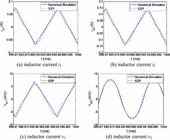
Comparison of ripples of state variables of Cuk in CCM
The analysis method for the steady-state periodic solution of the converter operating in discontinuous-conduction-mode (DCM) is similar and will not be repeated in this chapter. We can also refer to Chap. 6, which provides a detailed description of the steady-state periodic solution of a closed-loop converter operating in DCM.
4.6 Transient Analysis of the Open-Loop PWM Converter by ESPM
4.6.1 The Solution Procedure

![$${\mathbf{x}} = [x_{1} ,x_{2} , \cdots x_{l} ]^{Tr}$$](../images/419194_1_En_4_Chapter/419194_1_En_4_Chapter_TeX_IEq105.png) (the superscript “Tr” indicates matrix transposition). The l*l-ordered coefficient matrices
(the superscript “Tr” indicates matrix transposition). The l*l-ordered coefficient matrices  and
and  are all related to the differential operator
p and the circuit parameters, where the highest number of p is 1. The term
are all related to the differential operator
p and the circuit parameters, where the highest number of p is 1. The term  a input vector with l*1 order, and the l*l-ordered nonlinear vector function
  is related to the state variable vector
  .
.
 gives:

 is an approximate order;
  is a small parameter marker.
 and
and  in Eq. (4.82) for state variables x can be expressed in the Fourier series as follows
 , the terms
  and
and  are the conjugate plurals of
  and
and  respectively. It should be noted that, unlike the steady-state periodic solution, the harmonic coefficients
  and
and  are variables related to the normalized time
  . In the case of a steady-state periodic solution, the coefficients
  and
and  are unknown constants to be solved, they are independent of time. Similar to the solution of the steady-state periodic solution, in Eq. (4.85), the spectral set E0 of the principal component is determined by the physical knowledge associated with the system under study. For example, when the switching power converter system is stable, the main component of its output voltage and inductor current is DC, so
  can be selected; and for the weak nonlinear system we can choose
  , which means that only the fundamental wave are contained in the main component. The frequency set
  of the correction term
  is determined step by step during the iteration.
 into
into  and decomposing
  into the sum of the main term and the remainder, the following formula can be obtained.
 has the same spectral set as the term
  , that is, all items in
  with the same harmonic components as
  belong to
  , while other harmonic components belong to the remainder
  . Therefore,
  can be regarded as a small amount with higher order than the term
fim, and in front of which the small amount indicator
can be regarded as a small amount with higher order than the term
fim, and in front of which the small amount indicator  is introduced again. The terms
  and
and  can be expressed into Fourier series as follows:
![$${\mathbf{f}}_{0m} = \sum\limits_{{k \in E_{0} }} {\left[ {{\mathbf{h}}_{n0} (\tau )e^{jn\tau } + {\bar{\mathbf{h}}}_{n0} (\tau )e^{ - jn\tau } } \right] \, }$$](../images/419194_1_En_4_Chapter/419194_1_En_4_Chapter_TeX_Equ96.png)
![$${\mathbf{f}}_{im} = \sum\limits_{{k \in E_{i} }} {\left[ {{\mathbf{h}}_{ki} (\tau )e^{jk\tau } + {\bar{\mathbf{h}}}_{ki} (\tau )e^{ - jk\tau } } \right] \, }$$](../images/419194_1_En_4_Chapter/419194_1_En_4_Chapter_TeX_Equ97.png)
![$${\mathbf{R}}_{i + 1} = \sum\limits_{{k \in E_{i + 1} }} {\left[ {{\mathbf{h}}_{k(i + 1)}^{{\prime }} (\tau )^{jk\tau } + {\bar{\mathbf{h}}}_{k(i + 1)}^{{\prime }} (\tau )e^{ - jk\tau } } \right]}$$](../images/419194_1_En_4_Chapter/419194_1_En_4_Chapter_TeX_Equ98.png)
It still should be noted that, the amplitude coefficients of each harmonic in the above equations are time-dependent variables, which are quite different with those in the steady-state periodic solution.

 on both sides of the equation equal, you can get the following iterative equations as

 of the harmonic components with the steady-state solution, the differential operator
  in Eq. (3.43), where k = 0, 1 …, represents the order of harmonics.
 of the harmonic components are time-dependent variables, there exists the following equation about the differential operation.
![$$\begin{aligned} p[{\mathbf{a}}_{ki} (\tau )e^{jk\omega t} ] & = \frac{{d[{\mathbf{a}}_{ki} (\tau )e^{jk\omega t} ]}}{dt} = \frac{{d[{\mathbf{a}}_{ki} (\tau )]}}{dt} \cdot e^{jk\omega t} + jk\omega \cdot {\mathbf{a}}_{ki} (\tau )\,e^{jk\omega t} \\ & \,{ = }\, (p{ + }jk\omega ){\mathbf{a}}_{ki} (\tau )\,e^{jk\omega t} \\ \end{aligned}$$](../images/419194_1_En_4_Chapter/419194_1_En_4_Chapter_TeX_Equ102.png)
Therefore, when finding the coefficients  of the harmonic components with the transient solution, we use (p + jkω) instead of the differential operator p in Eq. (4.89).


 represents the initial values of the state variable vector.
4.6.2 Initial Value Determination

 = 1.
= 1.In the case of simple estimation,  can be used to obtain the transient solution
  of the first equation in Eq. (4.89), and then the forced solutions
  and
and  … of the second and the third equations in Eq. (4.89) …, etc. However, the transient solution obtained in this way usually does not satisfy the initial conditions (4.94).
- (1)
Let
 , and find
  by the first equation of Eq. (4.89);
 - (2)
Solve the second equation of Eq. (4.89) and get the special solution
 , then let
  ;
; - (3)
Similarly, after solving Eq. (4.89) to obtain the special solutions
 and
and  , …, etc., let
  . Then use the modified
  as the initial value to find
  , and according to the correction equation, the special solutions
  and
and  , …, etc. are obtained one by one, and finally the transient solution of Eq. (4.89) is obtained.
It must be noted that when using the equivalent small-parameter method, as long as the appropriate main component is selected, the initial  has little effect on the special solution
  . Thus, if
  is selected, then
  can be made to simplify the analysis process of the transient solution.
4.6.3 Transient Analysis of Open-Loop PWM Boost Converter
We still take the Boost converter shown in Fig. 4.1 as an example to illustrate the analysis of the transient solution of a switching converter using the ESPM. The circuit parameters are chosen as: L = 6 mH, C = 45 μF, R = 30 Ω, E = 37.5 V, fs = 1 kHz, and the duty ratio is set to be D = 0.25.

![$$G_{0} \left( p \right) = \left[ {\begin{array}{*{20}c} p & {\frac{1}{L}} \\ {\frac{ - 1}{C}} & {p + \frac{1}{RC}} \\ \end{array} } \right],\quad G_{1} \left( p \right) = \left[ {\begin{array}{*{20}c} 0 & {\frac{ - 1}{L}} \\ {\frac{1}{C}} & 0 \\ \end{array} } \right],\quad {\mathbf{u}} = \left[ {\begin{array}{*{20}c} {E/L} \\ 0 \\ \end{array} } \right]$$](../images/419194_1_En_4_Chapter/419194_1_En_4_Chapter_TeX_Equ107.png)

 is defined as shown in Eq. (4.12).
 , so the zero-order approximate solution can be assumed to be
![$${\mathbf{x}}_{0} = a_{00} (t) = \left[ {i_{00} ,v_{00} } \right]^{Tr}$$](../images/419194_1_En_4_Chapter/419194_1_En_4_Chapter_TeX_Equh.png)
![$$\left[ {{\mathbf{G}}_{0} (p) + {\mathbf{G}}_{1} (p)b_{0} } \right]{\mathbf{a}}_{00} (\tau ) = {\mathbf{u}}$$](../images/419194_1_En_4_Chapter/419194_1_En_4_Chapter_TeX_Equ109.png)
![$$\left( {\left[ {\begin{array}{*{20}c} p & {\frac{1}{L}} \\ { - \frac{1}{C}} & {p + \frac{1}{RC}} \\ \end{array} } \right] + \left[ {\begin{array}{*{20}c} 0 & { - \frac{{b_{0} }}{L}} \\ {\frac{{b_{0} }}{C}} & 0 \\ \end{array} } \right]} \right)\left[ {\begin{array}{*{20}c} {i_{00} } \\ {v_{00} } \\ \end{array} } \right] = \left[ {\begin{array}{*{20}c} {E/L} \\ 0 \\ \end{array} } \right]$$](../images/419194_1_En_4_Chapter/419194_1_En_4_Chapter_TeX_Equ110.png)

![$${\mathbf{A}}_{0} = \left[ {\begin{array}{*{20}c} 0 & { - \frac{1 - D}{L}} \\ {\frac{1 - D}{C}} & {\frac{ - 1}{RC}} \\ \end{array} } \right],\quad {\mathbf{u}} = \left[ {\begin{array}{*{20}c} {E/L} \\ 0 \\ \end{array} } \right]$$](../images/419194_1_En_4_Chapter/419194_1_En_4_Chapter_TeX_Equi.png)
![$$\begin{aligned} i_{00} & = 2.222 - {\text{e}}^{ - 0.059\tau } [2.222\,{ \cos }\,0.222\tau + 3.89\,{ \sin }\,0.222\tau ] \\ v_{00} & = 50 - {\text{e}}^{ - 0.059\tau } [50\,{ \cos }\,0.222\tau - 13.276\,{ \sin }\,0.222\tau ] \\ \end{aligned}$$](../images/419194_1_En_4_Chapter/419194_1_En_4_Chapter_TeX_Equ112.png)
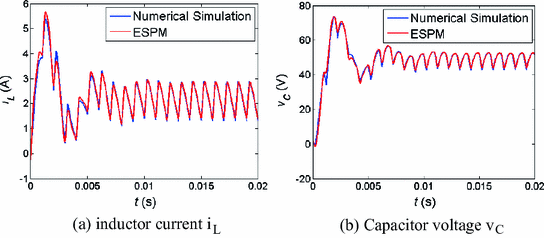
 . The results from Eq. (4.100) (red dashed line) and the simulations (green solid line) are compared in Fig. 4.11, from which it can be seen that the zero-order approximation roughly grasps the characteristics of the transient process.
Zero-order approximation of the transient solution of CCM-Boost converter

![$${\mathbf{a}}_{11} (t) = \left[ {i_{11} ,v_{11} } \right]^{Tr}$$](../images/419194_1_En_4_Chapter/419194_1_En_4_Chapter_TeX_IEq172.png) . By replacing (p + jω) with the (jω) in Eq. (4.35), the first-order correction equation corresponding to the second equation in Eq. (4.89) can be obtained as
. By replacing (p + jω) with the (jω) in Eq. (4.35), the first-order correction equation corresponding to the second equation in Eq. (4.89) can be obtained as![$$[{\mathbf{G}}_{0} (p + {\text{j}}\omega ) + {\mathbf{G}}_{1} (p + {\text{j}}\omega ){\text{b}}_{0} ]{\mathbf{a}}_{11} = - {\mathbf{G}}_{1} (p + {\text{j}}\omega ) \cdot b_{1} {\mathbf{a}}_{00}$$](../images/419194_1_En_4_Chapter/419194_1_En_4_Chapter_TeX_Equ113.png)
![$$\left( {\left[ {\begin{array}{*{20}c} {p + j\omega } & {\frac{1}{L}} \\ { - \frac{1}{C}} & {p + j\omega + \frac{1}{RC}} \\ \end{array} } \right] + \left[ {\begin{array}{*{20}c} 0 & { - \frac{D}{L}} \\ {\frac{D}{C}} & 0 \\ \end{array} } \right]} \right)\left[ {\begin{array}{*{20}c} {i_{11} } \\ {v_{11} } \\ \end{array} } \right] = \left[ {\begin{array}{*{20}c} 0 & {\frac{1}{L}} \\ {\frac{ - 1}{C}} & 0 \\ \end{array} } \right]\left[ {\begin{array}{*{20}c} {b_{1} i_{00} } \\ {b_{1} v_{00} } \\ \end{array} } \right]$$](../images/419194_1_En_4_Chapter/419194_1_En_4_Chapter_TeX_Equ114.png)

![$${\mathbf{A}}_{1} = \left[ {\begin{array}{*{20}c} { - j\omega } & { - \frac{1 - D}{L}} \\ {\frac{1 - D}{C}} & { - j\omega - \frac{1}{RC}} \\ \end{array} } \right],\quad {\mathbf{B}}_{1} = \left[ {\begin{array}{*{20}c} 0 & {\frac{{b_{1} }}{L}} \\ {\frac{{ - b_{1} }}{C}} & 0 \\ \end{array} } \right]$$](../images/419194_1_En_4_Chapter/419194_1_En_4_Chapter_TeX_Equk.png)
![$$\begin{aligned} i_{11} & = {\text{e}}^{ - 0.059\tau } [0.2209\,{\text{cos(}}0.222\tau ) + 0.2547\,{\text{sin(}}0.222\tau ) + 0.7298\,\cos (1.222\tau ) \\ & \quad - 0.1333\,\sin (1.222\tau )] - 0.5007\,\cos \tau + 0.4031\,\sin \tau \\ v_{11} & = {\text{e}}^{ - 0.059\tau } [ - 2.188\,{\text{cos(}}0.222\tau ) + 3.22\,{\text{sin(}}0.222\tau ) + 1.22\,\cos ( 1.222\tau ) \\ & \quad + 3.365\,\sin ( 1.222\tau )] + 0.968\,\cos \tau - 3.945\,\sin \tau \\ \end{aligned}$$](../images/419194_1_En_4_Chapter/419194_1_En_4_Chapter_TeX_Equ116.png)
![$${\mathbf{x}} \approx {\mathbf{x}}_{0} + {\mathbf{x}}_{1} = \left[ {\begin{array}{*{20}c} {i_{00} + i_{11} } \\ {v_{00} + v_{11} } \\ \end{array} } \right]$$](../images/419194_1_En_4_Chapter/419194_1_En_4_Chapter_TeX_Equ117.png)

First-order approximation of the transient solution of CCM-Boost converter
![$${\mathbf{x}} = [\begin{array}{*{20}c} {i_{L} } & {v_{C} } \\ \end{array} ]^{Tr} \approx {\mathbf{x}}_{0} + {\mathbf{x}}_{1} + {\mathbf{x}}_{2}$$](../images/419194_1_En_4_Chapter/419194_1_En_4_Chapter_TeX_Equ118.png)
![$$\begin{aligned} i_{L} & \approx 2.1734 + {\text{e}}^{ - 0.059\tau } [ - 2.1335\,{\text{cos(0}} . 2 2 2\tau ) + 4.1547\,{\text{sin(0}} . 2 2 2\tau ) + 0.021\tau \,{\text{cos(0}} . 2 2 2\tau ) \\ & \quad + 0.0018\tau \,\sin ( 0. 2 2 2\tau ) + 0.1810\,{ \cos }(0.778\tau ) - 0.0238\,\sin (0.778\tau ) \\ & \quad + 0.2733\,\cos (1.222\tau ) - 0.1333\,\sin (1.222\tau )] - 0.5007\,\cos \tau + 0.4031\,\sin \tau \\ & \quad - 0.2051\,\cos 2\tau - 0.002\,\sin 2\tau - 0.0476\,{ \cos }3\tau - 0.0408\,\sin 3\tau \\ \end{aligned}$$](../images/419194_1_En_4_Chapter/419194_1_En_4_Chapter_TeX_Equ119.png)
![$$\begin{aligned} v_{C} & \approx 49.368 + {\text{e}}^{ - 0.059\tau } [ - 51.636\,{\text{cos(0}} . 2 2 2\tau ) - 12.352\,{\text{sin(0}} . 2 2 2\tau ) \\ & \quad + 0.0438\tau \,{\text{cos(0}} . 2 2 2\tau ) + 0.2431\tau \,\sin ( 0. 2 2 2\tau ) + 0.0768\,{ \cos }(0.778\tau ) \\ & \quad + 0.2672\,\sin (0.778\tau ) + 1.22\,\cos (1.222\tau ) + 3.3648\,\sin (1.222\tau )] + 0.0968\,\cos \tau \\ & \quad - 3.945\,\sin \tau + 1. 2 3 9 7\,\cos 2\tau - 0.026\,\sin 2\tau + 0.1878\,{ \cos }3\tau + 0.3523\,\sin 3\tau \\ \end{aligned}$$](../images/419194_1_En_4_Chapter/419194_1_En_4_Chapter_TeX_Equ120.png)
Second-order approximation of the transient solution of CCM-Boost converter
4.6.4 Simplified Calculation

![$$\begin{aligned} i & \approx {\text{e}}^{ - 0.059\tau } [ - 2.222\,{ \cos }\,0.222\tau + 3.89\,{ \sin }\,0.222\tau ] + i_{steady} \\ v & \approx {\text{e}}^{ - 0.059\tau } [ - 50\,{ \cos }\,0.222\tau - 13.276\,{ \sin }\,0.222\tau ] + v_{steady} \\ \end{aligned}$$](../images/419194_1_En_4_Chapter/419194_1_En_4_Chapter_TeX_Equ122.png)

Approximated transient solution of CCM-Boost converter from simplified method
4.7 Summary
In this chapter, the equivalent-small-parameter method is used to analyze the PWM converters operating in CCM (continuous current mode) and DCM (discontinuous current mode) for obtaining the analytical expressions of steady-state periodic solutions and transient solutions. The equivalent-small-parameter method overcomes the shortcoming of dealing with large amount of calculation, which exists in the general average method. It is only necessary to solve the linear algebra or differential equations with lower order. It shows that even if the switching frequency is low and the ripple is large, the ESPM can still be applicable with high precision.