Over the course of a day, an individual makes many decisions that range from ones of great importance to ones of small consequence. A person is said to make a decision when buying a new car, when choosing to spend an evening with one friend rather than another, or when deciding what to eat for supper. Animals also make a variety of decisions; they may choose mates with particular characteristics, select one type of food over another, or decide to leave a territory.
From a behavioral view, the analysis of choice is concerned with the distribution of operant behavior among alternative sources of reinforcement (options). When several options are available, one alternative may be selected more frequently than others. When this occurs, it is called preference for an alternative source of reinforcement. For example, a person may choose between two food markets (a large supermarket and the corner store) on the basis of price, location, and variety. Each time the individual goes to one store rather than the other, she is said to choose. Eventually, the person may shop more frequently at the supermarket than the local grocery, and when this occurs the person is showing preference for the supermarket alternative.
Many people describe choosing to do something, or a preference for one activity over another, as a subjective experience. For example, you may simply like one person better than others, and based on this you feel good about spending a day with that person. From a behavioral perspective, your likes and feelings are real but they do not provide an objective scientific account of what you decide to do. To provide that account, it is necessary to identify the conditions that affected your attraction to (or preference for) the other person or friend.
For behavior analysts, the study of choice is based on principles of operant behavior. In previous chapters, operant behavior was analyzed in situations in which one response class was reinforced on a single schedule of reinforcement. For example, a child is reinforced with contingent attention from a teacher for correctly completing a page of arithmetic problems. The teacher provides one source of reinforcement (attention) when the child emits the target operant (math solutions). The single-operant analysis is important for the discovery of basic principles and applications. However, this same situation may be analyzed as a choice among behavioral options. The child may choose to do math problems or emit other behavior (e.g., look out of the window or talk to another child). This analysis of choice extends the operant paradigm or model to more complex environments in which several response and reinforcement alternatives are available.
In the everyday environment, there are many alternatives that schedule reinforcement for operant behavior. A child may distribute time and behavior among parents, peer group, and sport activities. Each alternative may require specific behavior and provide reinforcement at a particular rate and amount. To understand, predict, and change the child's behavior, all of these response-consequence relationships must be taken into account. Thus, the operant analysis of choice and preference begins to contact the complexity of everyday life, offering new principles for application.
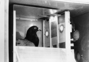
In the laboratory, choice and preference are investigated by arranging concurrent schedules of reinforcement (Catania, 1966). Figure 9.1 shows a concurrent two-key procedure for a pigeon. In the laboratory, two or more simple schedules (i.e., FR, VR, FI, or VI) are simultaneously available on different response keys (Ferster & Skinner, 1957). Each key is programmed with a separate schedule of reinforcement, and the organism is free to distribute behavior between the alternative schedules. The distribution of time and behavior among the response options is the behavioral measure of choice and preference. For example, a food-deprived bird may be exposed to a situation in which the left response key is programmed to deliver 20 presentations of the food hopper each hour, while the right key delivers 60 reinforcers an hour. To obtain reinforcement from either key, the pigeon must respond according to the schedule on that key. If the bird responds exclusively to the right key (and never to the left) and meets the schedule requirement, then 60 reinforcers will be delivered each hour. Because the bird could have responded to either side, we may say that it prefers to spend its time on the right alternative.
Concurrent schedules of reinforcement have received considerable research attention because they may be used as an analytical tool for understanding choice and preference. This selection of an experimental paradigm or model is based on the reasonable assumption that contingencies of reinforcement contribute substantially to choice behavior. Simply stated, all other factors being equal, the more reinforcement (higher rate) provided by an alternative, the more time and energy spent on that alternative. For example, in choosing between spending an evening with two friends, the one who has provided the most social reinforcement will probably be the one selected. Reinforcement may be social approval, affection, interesting conversation, or other aspects of the friend's behavior. The experience of deciding to spend the evening with one friend rather than the other may be something like, “I just feel like spending the evening with Fred.” Of course, in everyday life choosing is seldom as uncomplicated as this, and a more common decision might be to spend the evening with both friends. However, to understand how reinforcement processes are working, it is necessary to control the other factors so that the independent effects of reinforcement on choice may be observed.
FIG. 9.1 A two-key operant chamber for birds. Schedules of food reinforcement are arranged simultaneously on each key.
Figure 9.2 shows a two-key concurrent-operant setting for humans. Consider that you are asked to participate in an experiment in which you may earn up to $50 an hour. As an experimental participant, you are taken to a room that has two response keys separated by a distance of 8 ft. Halfway between the two keys is a small opening just big enough for your hand to fit. The room is empty, except for the unusual-looking apparatus. You are told to do anything you want. What do you do? You probably walk about and inspect your surroundings and, feeling somewhat foolish, eventually press one of the response keys. Immediately following this action, $1 is dispensed by a coin machine and is held on a plate inside the small opening. The dollar remains available for about 5 s, and then the plate falls away and the dollar disappears. Assuming that you have retrieved the dollar, will you press one of the keys again? In reality, this depends on several factors: perhaps you are wealthy and the dollar is irrelevant; perhaps you decide to “get the best of the experimenter” and show that you are not a rat; maybe you do not want to appear greedy; and so on. However, assume for the moment that you are a typical poor student and you press the key again. After some time pressing both keys and counting the number of key presses, you discover a rule. The left key pays a dollar for each 100 responses, while the right side pays a dollar for 250 responses. Does it make sense to spend your effort on the right key when you can make money faster on the other alternative? Of course it does not, and you decide to spend all of your work on the key that pays the most. This same result has been found with other organisms. When two ratio schedules (in this case FR 100 and FR 250) are programmed as concurrent schedules, the alternative that produces more rapid reinforcement is chosen exclusively (Herrnstein & Loveland, 1975).
Because ratio schedules result in exclusive responding to the alternative with the highest rate of payoff, these schedules are seldom used to study choice. We have discovered something about choice: Ratio schedules produce exclusive preference (see McDonald, 1988, on how to program concurrent ratio schedules to produce response distributions similar to those that occur on interval schedules). Although this result is interesting, it suggests that other schedules should be used to investigate choice and preference. Once exclusive responding occurs on ratio schedules, it is not possible to study how responses are distributed between the alternatives—the major objective for an experimental analysis of choice.
Consider, however, what you might do if interval schedules were programmed on the two response keys. Remember that on an interval schedule a single response must occur after a defined amount of time. If you spend all of your time pressing the same key, you will miss reinforcement that is programmed on the other alternative. For example, if the left key is scheduled to pay a dollar every 2 min and the right key every 6 min, then a reasonable tactic is to spend most of your time responding on the left key but every once in a while check out the other alternative. This behavior will result in obtaining most of the money set up by both schedules. In fact, when exposed to concurrent interval schedules, most animals
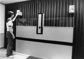
FIG. 9.2 A two-key operant chamber for humans. Pressing the keys results in money from a coin dispenser (middle), depending on the schedules of reinforcement.
distribute their time and behavior between the two alternatives in such a manner (de Villiers, 1977). Thus, the first prerequisite of the choice paradigm is that interval schedules must be used to study the distribution of behavior.
Interval schedules are said to be independent of one another when they are presented concurrently. This is because responding on one alternative does not affect the rate of reinforcement programmed for the other schedule. For example, a fixed-interval 6-min schedule (FI 6 min) is programmed to deliver reinforcement every 6 min. Of course, a response must be made after the fixed interval has elapsed. Pretend that you are faced with a situation in which the left key pays a dollar every 2 min (FI 2 min). The right key delivers a dollar when you make a response after 6 min. You have 1 h a day in the experiment. If you just respond to the FI 2-min schedule, you would earn approximately $30. On the other hand, you could increase the number of payoffs an hour by occasionally pressing the FI 6-min key. This occurs because the left key pays a total of $30 each hour and the right key pays an additional $10. After many hours of choosing between the alternatives, you may develop a stable pattern of responding. This steady-state performance is predictable. You should respond for approximately 6 min on the FI 2-min alternative and obtain three reinforcers ($3). After the third reinforcer, you may feel like switching to the FI 6-min key, on which a reinforcer is immediately available. You obtain the money on this key and immediately return to the richer schedule (left key). This steady-state pattern of responding may be repeated over and over with little variation.
Recall that there are two major types of interval schedules. On variable-interval schedules (VI), the time between each programmed reinforcer changes and the average time to reinforcement defines the specific schedule (VI 60 s). Because the organism is unable to discriminate the time to reinforcement on VI schedules, the regular switching pattern that characterizes concurrent FI FI performance does not occur. This is an advantage for the analysis of choice because the organism must respond on both alternatives as switching does not result always in reinforcement. Thus, operant behavior maintained by concurrent VI VI schedules is sensitive to the rate of reinforcement on each alternative. For this reason, VI schedules are typically used to study choice.
At this point, the choice paradigm is almost complete. Again, however, consider what you would do in the following situation. The two keys are separated and you cannot press both at the same time. The left key now pays a dollar on a VI 2-min schedule while responses to the right alternative are reinforced on VI 6 min. The left key pays $30 each hour, and the right one delivers $10 if you respond. Assuming you obtain all programmed reinforcers on both schedules, you earn $40 for each experimental session. What can you do to earn the most per hour? If you stay on the VI 2-min side, you end up missing the 10 reinforcers on the other alternative. However, if you frequently change over from key to key, most of the reinforcers on both schedules will be obtained. This is in fact what most animals do when faced with these contingencies (de Villiers, 1977).
Simple alternation between response alternatives prevents an analysis of choice because the distribution of behavior remains the same (approximately 50/50) no matter what the programmed rates of reinforcement. Frequent switching between alternatives may occur because of the correlation between rate of switching and overall rate of reinforcement (dollars per session). In other words, as the rate of switching increases, so does the hourly payoff. Another way of looking at this alternation is that organisms are accidentally reinforced for the changeover response. This alternation is called concurrent superstition (Catania, 1966) and occurs because as time is spent on one alternative, the other schedule is timing out. As the organism spends more time on the left key, the probability of a reinforcer being set up on the right key increases. This means that a changeover to the right alternative will be reinforced even though the contingencies do not require the changeover response. Thus, switching to the other response key is an operant that is inadvertently strengthened.
The control procedure used to stop rapid switching between alternatives is called a changeover delay, or COD (Shull & Pliskoff, 1967). The COD contingency stipulates that responses will not have an effect immediately following a change from one schedule to another. After switching to a new alternative, a brief time is required before a response can be reinforced (e.g., 3-s delay). For example, if an organism has just changed to an alternative that is ready to deliver reinforcement, there is a 3-s delay before a response is effective. As soon as the 3-s delay has elapsed, a response is reinforced. Of course, if the schedule has not timed out, the COD is irrelevant because reinforcement is not yet available. The COD contingency operates in both directions whenever a change is made from one alternative to another. The COD prevents frequent switching between alternatives. To obtain reinforcement, an organism must spend a minimal amount of time on an alternative before switching to another schedule. For example, with a 3-s COD, changing over every 2 s will never result in reinforcement. The COD is therefore an important and necessary feature of the operant-choice procedure.
The basic paradigm for investigating choice and preference is now complete. In summary, a researcher interested in behavioral choice should:
1. Arrange two or more concurrently available schedules of reinforcement.
2. Program interval schedules on each alternative.
3. Use variable- rather than fixed-interval schedules.
4. Require a COD in order to stop frequent alternation between or among the schedules.
Findley (1958) described an interesting variation on the basic choice procedure. The Findley procedure involves a single response key that changes color. Each color is a stimulus that signals a particular schedule of reinforcement. The color and the programmed schedule may be changed by a response to a second key. This key is called the changeover key. For example, a pigeon may respond on a VI 30-s schedule that is signaled by red illumination of the response key. When the bird pecks a second changeover key, the color on the response key changes from red to blue and a new schedule is operative. In the presence of the blue light, the pigeon may respond on a VI 90-s schedule of reinforcement. Another response on the changeover key reinstates the red light and the VI 30-second schedule. The advantage of the Findley procedure is that the response of changing from one alternative to another is explicitly defined and measured. Figure 9.3 compares the two-key and Findley procedures, showing that the Findley method allows for the measurement and control of the changeover response.
FIG. 9.3 Comparison of two-key and Findley procedures. Notice that the Findley method highlights the changeover response.
Current evidence suggests that the same principles of choice account for behavior in both the two-key and changeover procedures. For this reason, researchers have not made a theoretical distinction between them. However, such a distinction may be important for the analysis of human behavior. Sunahara and Pierce (1982) suggested that the two-key procedure provides a model for social interaction. For example, in a group discussion a person may distribute talk and attention to several group members. These members may be viewed as alternative sources of social reinforcement for the person. On the other hand, the changeover-key procedure may model role taking, in which an individual responds differentially to the role of another person. In this case, the individual may change over between the reinforcement schedules provided by the other person as a friend or as a boss. For example, while at work the changeover may be made by saying, “Could I discuss a personal problem with you?” In other words, a person who is both your friend and supervisor at work may sometimes deliver social reinforcement as a friend and at other times as your boss. Your behavior changes when the other person provides differential reinforcement in these two different roles.
In 1961, Richard Herrnstein (Figure 9.4) published an influential paper that described the distribution of behavior on concurrent schedules of positive reinforcement. He found that pigeons matched relative rates of behavior to relative rates of reinforcement. For example, when 90% of the total reinforcement was provided by schedule A (and 10% by schedule B), approximately 90% of the bird's key pecks were on the A schedule. This equality or matching between relative rate of reinforcement and relative rate of response is known as the matching law. To understand this law, we turn to Herrnstein's (1961b) experiment.

FIG. 9.4 Richard Herrnstein. Reprinted with permission.
In this study, Herrnstein investigated the behavior of pigeons on a two-key concurrent schedule. Concurrent VI VI schedules of food reinforcement were programmed with a 1.5-s COD. The birds were exposed to different pairs of concurrent variable-interval schedules for several days. Each pair of concurrent schedules was maintained until response rates stabilized. That is, behavior on each schedule did not significantly change from session to session. After several days of stable responding, a new pair of schedule values was presented. Overall rate of reinforcement was held constant at 40 reinforcers per hour for all pairs of schedules. Thus, if the schedule on the left key was programmed to deliver 20 reinforcers an hour (VI 3 min), then the right key also provided 20 reinforcers. If the left key supplied 10 reinforcers, then the right key supplied 30 reinforcers. The schedule values that Herrnstein used are presented in Figure 9.5.
The data in Figure 9.5 show the schedules operating on the two keys, A and B. As previously stated, the total number of scheduled reinforcers is held constant for each pair of VI schedules. This is indicated in the third column, in which the sum of the reinforcements per hour (Rft/h) is equal to 40 for each set of schedules. Because the overall rate of reinforcement remains constant, changes in the distribution of behavior cannot be attributed to this factor. Note that when key A is programmed to deliver 20 reinforcers an hour, so is key B. When this occurs, the responses per hour (Rsp/h) are the same on each key. However, the responses per hour (or absolute rate) are not the critical measure of preference. Recall that choice and preference are measured as the distribution of time or behavior between alternatives. To express the idea of distribution, it is important to direct attention to relative measures. Because of this, Herrnstein focused on the relative rates of response. In Figure 9.5, the relative rate of response is expressed as a proportion. That is, the rate of response on key A is the numerator and the sum of the response rates on both keys is the denominator. The proportional rate of response on key A is shown in the final column, labeled “Relative responses.”
FIG. 9.5 A table of schedule values and data. Reinforcement per hour (Rft/h), responses per hour (Rsp/h), relative reinforcement (proportions), and relative responses (proportions) are shown. Adapted from Fig. 1 (bird 231) and text of “Relative and Absolute Strength of Responses as a Function of Frequency of Reinforcement,” by R. J. Herrnstein, 1961b, Journal of the Experimental Analysis of Behavior, 4, 267–272.
To calculate the proportional rate of responses to key A for the pair of schedules VI 4.5 min VI 2.25 min, the following simple formula is used:
Ba/(Ba + Bb)
The term Ba is behavior measured as the rate of response on key A, or 1750 pecks per hour. Rate of response on key B is 3900 pecks per hour and is represented by the term Bb term. Thus, the proportional rate of response on key A is
1750/(1750 + 3900) = 0.31
In a similar fashion, the proportion of reinforcement on key A may be calculated as
Ra/(Ra + Rb)
The term Ra refers to the scheduled rate of reinforcement on key A, or 13.3 reinforcers per hour. Rate of reinforcement on key B is designated by the term Rb and is 26.7 reinforcers each hour. The proportional rate of reinforcement on key A is calculated as
13.3/(13.3 + 26.7) = 0.33
These calculations show that the relative rate of response (0.31) is very close to the relative rate of reinforcement (0.33). If you compare these values for the other pairs of schedules, you will see that the proportional rate of response approximates the proportional rate of reinforcement.
Figure 9.5 shows that Herrnstein manipulated the independent variable, relative rate of reinforcement on key A, over a range of values. Because there are several values of the independent variable and a corresponding set of values for the dependent variable, it is possible to plot the relationship. Figure 9.6 shows the relationship between proportional rate of reinforcement, Ra/ (Ra + Rb) and proportional rate of response Ba/(Ba + Bb) for pigeon 231 based on the values in Figure 9.5.
Herrnstein showed that the major dependent variable in choice experiments was relative rate of response. He also found that relative rate of reinforcement was the primary independent variable. Thus, in an operant-choice experiment, the researcher manipulates the relative rate of reinforcement on each key and observes the relative rate of response to the respective alternatives.
FIG. 9.6 Proportional matching of the response and reinforcement rates for bird 231. Figure is based on results from Herrnstein (1961b) and the data reported in Figure 9.5.
As relative rate of reinforcement increases, so does the relative rate of response. Further, for each increase in relative reinforcement there is about the same increase in relative rate of response. This equality of relative rate of reinforcement and relative rate of response is expressed as a proportion in Equation (9.1):

Notice we have simply taken the Ba/(Ba + Bb) and the Ra/(Ra + Rb) expressions, which give the proportion of responses and reinforcers on key A, and mathematically stated that they are equal. In verbal form, we are stating that relative rate of response matches (or equals) relative rate of reinforcement. This statement, whether expressed verbally or mathematically, is known as the matching law.
In Figure 9.6, matching is shown as the solid black line. Notice that this line results when the proportional rate of reinforcement exactly matches the proportional rate of response. The matching law is an ideal representation of choice behavior. The actual data from pigeon 231 approximates the matching relationship. Herrnstein (1961b) also reported the results of two other pigeons that were well described by the matching equation.
The equality of rates of response and reinforcement is called a law of behavior because it describes how a variety of organisms choose among alternatives (de Villiers, 1977). Animals such as pigeons (Davison & Ferguson, 1978), wagtails (Houston, 1986), cows (Matthews & Temple, 1979), and rats (Poling, 1978) have demonstrated matching in choice situations. Interestingly, this same law applies to humans in a number of different settings (Bradshaw & Szabadi, 1988; Pierce & Epling, 1983). Reinforcers have ranged from food (Herrnstein, 1961b) to points that are subsequently exchanged for money (Bradshaw, Ruddle, & Szabadi, 1981). Behavior has been as diverse as lever pressing by rats (Norman & McSweeney, 1978) and conversation in humans (Conger & Killeen, 1974; Pierce, Epling, & Greer, 1981). Environments in which matching has been observed have included T-mazes, operant chambers, and open spaces with free-ranging flocks of birds (Baum, 1974a), as well as discrete-trial and free operant choice by human groups (Madden, Peden, & Yamaguchi, 2002). Also, special education students have been found to spend time on math problems proportional to the relative rate of reinforcement (e.g., Mace, Neef, Shade, & Mauro, 1994). Thus, the matching law describes the distribution of individual (and group) behavior across species, types of response, different reinforcers, and a variety of settings.
An interesting test of the matching law was reported by Conger and Killeen (1974). These researchers assessed human performance in a group discussion situation. A group was composed of three experimenters and one experimental participant. The participant was not aware that the other group members were confederates in the experiment and was asked to discuss attitudes toward drug abuse. One of the confederates prompted the participant to talk. The other two confederates were assigned the role of an audience. Each listener reinforced the subject's talk with brief positive words or phrases when a hidden cue light came on. The cue lights were scheduled so that the listeners gave different rates of reinforcement to the speaker. When the results for several participants were combined, relative time spent talking to the listener matched relative rate of agreement from the listener. These results suggest that the matching law operates in everyday social interaction.
In the laboratory, the matching relationship between relative rate of reinforcement and relative rate of response does not always occur. Figure 9.7 shows idealized patterns of departure from the matching law based on the proportion equation. The matching line is the dashed line going through the middle of the graphs. This line shows that when .5 of the reinforcements are on the left key then .5 of the responses are on this key, and when .75 of the reinforcements are obtained from the left side then .75 of responses are distributed to the left alternative. The first departure from ideal matching is called undermatching (Figure 9.7A). Notice that the response proportions are less sensitive to changes in the reinforcement proportions. In the case of undermatching, when relative rate of reinforcement is .75 the relative rate of response is only .55—it takes a large change in relative rate of reinforcement to produce a small change in relative behavior. The opposite of undermatching is called overmatching (Figure 9.7B), in which the response proportions are more extreme than reinforcement proportions. Research evidence suggests that undermatching is observed more often than overmatching (deVilliers, 1977). Figure 9.7C portrays a third kind of departure from matching known as response bias. In this case, the animal consistently spends more behavior on one alternative than predicted by the matching equation. The graph of response bias illustrates a situation where the pigeon spends more time on the right key than is expected by the matching relationship. Such bias indicates a systematic condition that affects preference other than the relative rate of reinforcement. For example, a pigeon may prefer the green key on the right compared to red on the left if the bird has a history of differential reinforcement in the presence of green.
In the complex world of people and other animals, departures from matching frequently occur (Baum, 1974b). This is because in complex environments, contingencies of positive and negative reinforcement may interact, reinforcers differ in value, and histories of reinforcement are not controlled. In addition, discrimination of alternative sources of reinforcement may be weak or absent. For example, pretend you are talking to two people after class at the local bar and grill. You have a
FIG. 9.7 Idealized graphs of undermatching (A), overmatching (B), and response bias (C), as would occur with the proportional matching equation. See text for details.
crush on one of these two and the other you do not really care for. Both of these people attend to your conversation with equal rates of social approval, eye contact, and commentary. You can see that even though the rates of reinforcement are the same, you will probably spend more time talking to the person you like best (response bias). Because this is a common occurrence in the nonlaboratory world, you might ask, “What is the use of matching and how can it be a law of behavior?”
The principle of matching is called a law because it describes the regularity underlying choice. Many scientific laws work in a similar fashion. Anyone who has an elementary understanding of physics can tell you that objects of equal mass fall to the earth at the same rate. Observation, however, tells you that a pound of feathers and a pound of rocks do not fall at the same velocity. We can only see the lawful relations between mass and rate of descent when other conditions are controlled. In a vacuum, a pound of feathers and a pound of rocks fall at equal rates and the law of gravity is observed. Similarly, with appropriate laboratory control, relative rate of response matches relative rate of reinforcement (see ADVANCED SECTION for more on departures from matching).
Behavioral choice can also be measured as time spent on an alternative (Baum & Rachlin, 1969; Brownstein & Pliskoff, 1968). Time spent is a useful measure of behavior when the response is continuous, as in talking to another person. In the laboratory, rather than measure the number of responses, the time spent on an alternative may be used to describe the distribution of behavior. The matching law can also be expressed in terms of relative time spent on an alternative. Equation (9.2) is similar to Equation (9.1) but states the matching relationship in terms of time:

In this equation, the time spent on alternative A is represented by Ta and the time spent on alternative B is Tb. Again, Ra and Rb represent the respective rates of reinforcement for these alternatives. The equation states that relative time spent on an alternative equals relative rate of reinforcement from that alternative. This extension of the matching law to continuous responses, such as standing in one place or looking at objects is important. Most behavior outside of the laboratory does not occur as discrete responses. In this case, Equation (9.2) may be used to describe choice and preference.
A consideration of either Equation (9.1) or Equation (9.2) makes it evident that to change behavior the rate of reinforcement for the target response may be adjusted; alternatively, the rate of reinforcement for other concurrent operants may be altered. Both of these procedures manipulate the relative rate of reinforcement for the specified behavior. Equation (9.3) represents relative rate of response as a function of several alternative sources of reinforcement:

In the laboratory, most experiments are conducted with only two concurrent schedules of reinforcement. However, the matching law also describes situations in which an organism may choose among several sources of reinforcement (Davison & Hunter, 1976; Elsmore & McBride, 1994; Miller & Loveland, 1974; Pliskoff & Brown, 1976). In Equation (9.3), behavior allocated to alternative A (Ba) is expressed relative to the sum of all behavior directed to the known alternatives (Ba + Bb + … Bn). Reinforcement provided by alternative A (Ra) is stated relative to all known sources of reinforcement (Ra + Rb + … Rn). Again, notice that an equality of proportions (matching) is stated.
The matching law has practical implications. A few researchers have shown that the matching equations are useful in applied settings (Borrero & Vollmer, 2002; Epling & Pierce, 1983; McDowell, 1981, 1982, 1988; Myerson & Hale, 1984; Plaud, 1992). One applied setting where the matching law has practical importance is the classroom, where students' behavior often is maintained on concurrent schedules of social reinforcement.
In a classroom, appropriate behavior for students includes working on assignments, following instructions, and attending to the teacher. In contrast, yelling and screaming, talking out of turn, and throwing paper airplanes are usually viewed as undesirable. All of these activities, appropriate or inappropriate, are presumably maintained by teacher attention, peer approval, sensory stimulation, and other sources of reinforcement. However, the schedules of reinforcement maintaining behavior in complex settings like a classroom are usually not known. When the objective is to increase a specific operant and the concurrent schedules are unknown, Myerson and Hale (1984) recommend the use of VI schedules to reinforce target behavior.
Recall that on concurrent ratio schedules, exclusive preference develops for the alternative with the higher rate of reinforcement (Herrnstein & Loveland, 1975). Ratio schedules are in effect when a teacher implements a grading system based on the number of correct solutions for assignments. The teacher's intervention will increase the students' on-task behavior only if the rate of reinforcement by the teacher is higher than another ratio schedule controlling inappropriate behavior. Basically, an intervention is either completely successful or a total failure when ratio schedules are used to modify behavior. In contrast, interval schedules of reinforcement will always redirect behavior to the desired alternative, although such a schedule may not completely eliminate inappropriate responding.
When behavior is maintained by interval contingencies, interval schedules remain the most desirable method for behavior change. Myerson and Hale (1984) used the matching equations to show that behavior-change techniques based on interval schedules are more effective than ratio interventions. They stated that “if the behavior analyst offers a VI schedule of reinforcement for competing responses two times as rich as the VI schedule for inappropriate behavior, the result will be the same as would be obtained with a VR schedule three times as rich as the schedule for inappropriate behavior” (pp. 373–374). Generally, behavior change will be more predictable and successful if interval schedules are used to reinforce appropriate behavior.
One of the fundamental problems of evolutionary biology and behavioral ecology concerns the concept of “optimal foraging” of animals (Krebs & Davies, 1978). Foraging involves prey selection where prey can be either animal or vegetable. Thus, a cow taking an occasional mouthful of grass in a field and a redshank wading in the mud and probing with its beak for an occasional worm are examples of foraging behavior. Because the function of foraging is finding food, foraging can be viewed as operant behavior regulated by food reinforcement. The natural contingencies of foraging present animals with alternative sources of food called patches. Food patches provide items at various rates (patch density) and in this sense are similar to concurrent schedules of reinforcement arranged in the laboratory.
Optimal foraging is said to occur when animals obtain the highest overall rate of reinforcement from their foraging. That is, over time organisms are expected to select between patches so as to optimize (obtain the most possible value from) their food resources. In this view, animals are like organic computers comparing their behavioral distributions with overall outcomes and stabilizing on a response distribution that ensures maximization of the overall rate of reinforcement.
In contrast to the optimal foraging hypothesis, Herrnstein (1982) proposed a process of melioration (doing the best at the moment). Organisms, he argued, are sensitive to fluctuations in the momentary rates of reinforcement rather than to long-term changes in overall rates of reinforcement. That is, an organism remains on one schedule until the local rates of reinforcement decline relative to that offered by a second schedule. Herrnstein (1997, pp. 74–99) showed that the steady-state outcome of the process of melioration is the matching law where relative rate of response matches relative rate of reinforcement. Thus, in a foraging situation involving two patches, Herrnstein's melioration analysis predicts matching of the distributions of behavior and reinforcement (e.g., Herrnstein & Prelec, 1997). Optimal foraging theory, on the other hand, predicts maximization of the overall rate of reinforcement (Charnov, 1976; Nonacs, 2001).
It is not possible to examine all the evidence for melioration, matching, and maximizing in this chapter, but Herrnstein (1982) has argued that melioration and matching are the basic processes of choice. That is, when melioration and matching are tested in choice situations that distinguish matching from maximizing, matching theory has usually predicted the actual distributions of the behavior.
One example of the application of matching theory to animal foraging is reported by Baum (1974a; see also Baum, 1983, on foraging) for a flock of free-ranging wild pigeons. The subjects were 20 pigeons that lived in a wooden frame house in Cambridge, Massachusetts. An opening allowed them to freely enter and leave the attic of the house. An operant apparatus with a platform was placed in the living space opposite to the opening to the outside. The front panel of the apparatus contained three translucent response keys and, when available, an opening allowed access to a hopper of mixed grain. Pigeons were autoshaped to peck to the center key and, following this training, a perch replaced the platform so that only one pigeon at a time could operate the keys and obtain food. Pigeons were now shaped to peck the center key on a VI 30-s schedule of food reinforcement. When a stable performance occurred, the center key was no longer illuminated or operative, and the two side keys became active. Responses to the illuminated side keys were reinforced on two concurrent VI VI schedules. Relative rates of reinforcement on the two keys were varied and the relative rate of response was measured.
Although only one bird at a time could respond on the concurrent schedules of reinforcement, Baum (1974b) treated the aggregate pecks of the group as the dependent measure. When the group of 20 pigeons chose between the two side keys, each of which occasionally produced food, the ratio of pecks to these keys approximately equaled the ratio of grain presentations obtained from them. That is, the aggregate behavior of the flock of 20 pigeons was in accord with the generalized matching equation, a form of matching equation based on ratios rather than proportions (see ADVANCED SECTION). This research suggests that the matching law applies to the behavior of wild pigeons in natural environments. Generally, principles of choice based on laboratory experiments can predict the foraging behavior of animals in the wild.
Choice and concurrent schedules of reinforcement have been analyzed from a microeconomic point of view (Rachlin, Green, Kagel, & Battalio, 1976). Behavioral economics involves the use of basic economic concepts and principles (law of demand, price, and substitutability) to analyze, predict, and control behavior in choice situations. One of the more interesting areas of behavioral economics concerns laboratory experiments that allow animals to work for drugs such as alcohol, heroin, and cocaine. For example, Nader and Woolverton (1992) showed that a monkey's choice of cocaine over food was a function of drug dose, but that choosing cocaine decreased as the price (number of responses per infusion) increased. That is, the reinforcing effects of the drug increased with dose but these effects were modified by price, an economic factor. In another experiment, Carroll, Lac, and Nygaard (1989) examined the effects of a substitute commodity on the use of cocaine. Rats nearly doubled their administration of cocaine when water was the other option than when the option was a sweet solution. These effects were not found in a control group that self-administered an inert saline solution, suggesting that cocaine infusion functioned as reinforcement for self-administration and that the sweet solution substituted for cocaine. Again, the reinforcing effects of the drug were altered by an economic factor, in this case the presence of a substitute commodity (see Carroll, 1993, for similar effects with monkeys and the drug PCP).
The concept of substitute commodities (reinforcers) may be useful in understanding the treatment of heroin addicts with methadone. From an economic perspective, methadone is a partial substitute for heroin because it provides only some of the reinforcing effects of the actual drug. Also, methadone is administered in a clinical setting that is less reinforcing than the social context in which heroin is often used (Hursh, 1991). Based on this analysis, it is unlikely that availability of methadone treatment will, by itself, eliminate the use of heroin.
To reduce drug abuse, Vuchinich (1999) suggests a multifaceted approach that (1) increases the cost of using drugs by law enforcement that reduces the supply (i.e., price goes up), (2) provides easy access to other, nondrug activities (e.g., sports, musical entertainment, etc.) and arranges reinforcement from family, friends, and work for staying drug free, and (3) provides reinforcement for nondrug behavior promptly, as delayed reinforcement is ineffective. These principles can be applied to many behavior problems, including smoking, use of alcohol, and compulsive gambling (Bickel & Vuchinich, 2000). It is no longer necessary or sensible to treat people as if they had an underlying illness or disease (e.g., alcoholism). Behavioral economics and learning principles offer direct interventions to modify excessive or addictive behavior.
Activity anorexia occurs when rats are placed on food restriction and provided with the opportunity to run. The initial effect is that food intake is reduced, body weight declines, and wheel running increases. As running escalates, food intake drops off and body weight plummets downward, further augmenting wheel running and suppressing food intake. The result of this cycle is emaciation and, if allowed to continue, the eventual death of the animal (Epling & Pierce, 1992, 1996b; Epling, Pierce, & Stefan, 1983; Routtenberg & Kuznesof, 1967).
A behavioral economic model can describe the allocation of behavior between commodities such as food and wheel running. For example, the imposed food restriction that initiates activity anorexia can be conceptualized as a substantial increase in the price of food, resulting in reduced food consumption. Low food consumption, in turn, increases consumption of physical activity— suggesting that food and physical activity may be economic substitutes (see Green & Freed, 1993, for a review of behavioral economic concepts).
In two experiments, Belke, Pierce, and Duncan (2006) investigated how animals choose between sucrose (food) and wheel running reinforcement. Rats were exposed to concurrent VI 30-s VI 30-s schedules of wheel running and sucrose reinforcement. Sucrose solutions varied in concentration: 2.5, 7.5, and 12.5%. As concentration increased, more behavior was allocated to sucrose and more reinforcements were obtained from that alternative. Allocation of behavior to wheel running decreased somewhat, but the obtained wheel-running reinforcement did not change. The results suggested that food-deprived rats were sensitive to changes in food supply (sucrose concentration) while continuing to engage in physical activity (wheel running). In the second study, rats were exposed to concurrent variable ratio (VR VR) schedules of sucrose and wheel running, wheel running and wheel running, and sucrose and sucrose reinforcement. For each pair of reinforcers, the researchers assessed substitutability by changing the prices for consumption of the commodities. Results showed that sucrose substituted for sucrose, and wheel running substituted for wheel running, as would be expected. Wheel running, however, did not substitute for sucrose—the commodities were independent; but sucrose partially substituted for wheel running.
The partial substitutability of sucrose for wheel running in the Belke et al. (2006) experiments reflects two energy-balance processes: the initiation and maintenance of travel induced by loss of body weight and energy stores (wheel running does not substitute for food) and the termination of locomotion as food supply increases (food does substitute for wheel running). In terms of activity anorexia, the fact that travel does not substitute for food insures that animals with low energy stores keep going on a food-related trek—even if they eat small bits along the way. As animals contact stable food supplies, the partial substitutability of food for wheel running means that travel would subside as food intake and body stores return to equilibrium. Behavioral economics therefore provides one way to understand the activity anorexia cycle.
Students often face the choice of going out to party or staying home and “hitting the books.” Often, when given the options, students pick the immediate reward of partying with friends over the delayed benefits of studying, learning the subject matter, and high grades. When a person (or other animal) selects the smaller, immediate payoff over the larger, delayed benefits, we may say that he/ she shows impulsive behavior. On the other hand, a person who chooses the larger, delayed reward while rejecting the smaller, immediate payoff is said to show self-control behavior. In term of a student's choices to party or study, choosing to party with friends is impulsive behavior while choosing to stay home and study is self-control behavior.
One of the interesting things about self-control situations is that our preferences change over time. That is, we may value studying over partying a week before the party, but value partying when the night of the party arrives. Howard Rachlin (1970, 1974) and George Ainslie (1975) independently suggested that these preference reversals could be analyzed as changes in reinforcement effectiveness with increasing delay. The Ainslie—Rachlin principle states that reinforcement value decreases as the delay between making a choice and obtaining the reinforcer increases (see top panel of Figure 9.8).
FIG. 9.8 An application of the Ainslie—Rachlin principle. The top panel shows that the reinforcement value of studying declines the farther the student is from the benefits obtained at the end of term. In the lower panel, the value of studying is lower than going to the party at the night of the party. However, the value of going to the party declines below the value of studying a week before the party. That is, the student's preference reverses.
As shown in Figure 9.8 (lower panel), the value of studying on the Friday night of the party (choice point) is lower than having fun with friends (partying) because the payoffs for studying (learning and good grades) are delayed until the end of the term. But if we move back in time from the choice point to a week before the party, the value of studying relative to partying reverses. That is, adding delay to each reinforcement option before a choice is made reverses the value of the alternative reinforcers. More generally, at some time removed from making a choice, the value of the smaller, immediate reinforcer will be less than the value of the larger, delayed reward, indicating a preference reversal. When preference reversal occurs, people (and other animals) will make a commitment response to forego the smaller, immediate reward and lock themselves into the larger, delayed payoff (see Chapter 13, section on Training Self-Control). Figure 9.9 shows the commitment procedure for eliminating the choice between studying and partying a week before the party. The commitment response is some behavior emitted at a time prior to the choice point that eliminates or reduces the probability of impulsive behavior. A student who has invited a classmate over to study on the Friday night of the party (commitment response) insures that she will “hit the books” and give up partying when the choice arrives.
Preference reversal and commitment occur over extended periods in humans and involve many complexities (e.g., Green, Fry, & Myerson, 1994; Logue, Pena-Correal, Rodriguez, & Kabela, 1986). In animals, delays of reinforcement by a few seconds can change the value of the options, instill
FIG. 9.9 Example of self-control through commitment based on preference reversal, as required by the Ainslie—Rachlin principle (as in Figure 9.8). The student will make a commitment to study at point A (a week before the party) because the value of studying is higher than partying, but not at the choice point B (the night of the party). The commitment response removes going to the party as an option on the night of the party (C).
commitment, and insure self-control over impulsiveness. As an example of preference reversal, consider an experiment by Green, Fisher, Perlow, and Sherman (1981) where pigeons responded on two schedules of reinforcement, using a trials procedure. The birds were given numerous trials each day. On each trial a bird made its choice by pecking one of two keys. A single peck at the red key resulted in 2 s of access to grain, while a peck at the green key delivered 6 s of access to food. The intriguing aspect of the experiment involved adding a brief delay between a peck and the delivery of food. In one condition, there was a 2-s delay for the 2-s reinforcer (red key) and a 6-s delay for 6-s access to food (green key). The data indicated that birds were impulsive, choosing the 2-s reinforcer on nearly every trial and losing about two-thirds of their potential access to food.
In another procedure, 18 additional seconds were added to the delays for each key so that the delays were now 20 s for the 2-s reinforcer and 24-s for the 6-s access to food. When the birds were required to choose this far in advance, they pecked the green key that delivered 6-s of access to food on more than 80% of the trials. In other words, the pigeons showed preference reversal and self-control when both reinforcers were farther away.
Other research by Ainslie (1974) and Rachlin and Green (1972) shows that pigeons can learn to make a commitment response, thereby reducing the probability of impulsive behavior. Generally, animal research supports the Ainslie—Rachlin principle and its predictions. One implication is that changes in reinforcement value over extended periods also regulate self-control and impulsiveness in humans (see Ainslie, 2005; Rachlin, 2000; Rachlin & Laibson, 1997). In this way, behavior principles may help to explain the impulsive use of credit cards in our society and the fact that most people have trouble saving their money (self-control).
The matching law suggests that operant behavior is determined by rate of reinforcement for one alternative relative to all other known sources of reinforcement. Even in situations in which a contingency exists between a single response and a reinforcement schedule, organisms usually have several reinforced alternatives that are unknown to the researcher. Also, many of the activities that produce reinforcement are beyond experimental control. A rat that is lever pressing for food may gain additional reinforcement from exploring the operant chamber, scratching itself, or grooming. In a similar fashion, rather than work for teacher attention, a pupil may look out of the window, talk to a friend, or even daydream. Thus, even in a single-operant setting, multiple sources of reinforcement are operating. Richard Herrnstein (1970, 1974) argued this point and suggested that all operant behavior must be understood as behavior emitted in the context of other alternative sources of reinforcement.
Based on these ideas, Herrnstein proposed a matching equation that describes the absolute rate of response on a single schedule of reinforcement. This mathematical formulation is called the quantitative law of effect. The law states that the absolute rate of response on a schedule of reinforcement is a hyperbolic function of rate of reinforcement on the schedule relative to the total rate of reinforcement, both scheduled and extraneous reinforcement. That is, as the rate of reinforcement on the schedule increases, the rate of response rapidly rises, but eventually further increases in rate of reinforcement produce less and less of an increase in rate of response (a hyperbolic curve; see Figure 9.10 for examples).
The rapid rise in rate of response with higher rates of reinforcement is modified by extraneous sources of reinforcement. Extraneous sources of reinforcement include any unknown contingencies that support the behavior of the organism. For example, a rat that is pressing a lever for food on a particular schedule of reinforcement could receive extraneous reinforcement for scratching, sniffing, and numerous other behaviors. The rate of response for food will be a function of the programmed schedule as well as the extraneous schedules controlling other behavior. In humans, a student's mathematical performance will be a function of the schedule of correct solutions as well as extraneous reinforcement for other behavior from classmates or teachers, internal neurochemical processes, and changes to the physical/chemical environment (e.g., smell of food drifting from the cafeteria).
Extraneous reinforcement slows down the rise in rate of response with higher rates of reinforcement. One implication is that control of behavior by a schedule of reinforcement is reduced as the sources of extraneous reinforcement increase. A student who does math problems for a given rate of teacher attention will do less if extraneous reinforcement is available by looking out of the window of the classroom. Alternatively, the teacher will have to use higher rates of attention for problem solving when “distractions” are available than when there are few additional sources of reinforcement.
The quantitative law of effect has been investigated in laboratory experiments. In an early investigation, Catania and Reynolds (1968) conducted an exhaustive study of six pigeons that pecked a key for food on different variable-interval (VI) schedules. Rate of reinforcement ranged from 8 to 300 food presentations each hour. Herrnstein (1970) replotted the data on X and Y coordinates. Figure 9.10 shows the plots for the six birds, with reinforcements per hour on the X-axis and responses per minute on the Y-axis.
Herrnstein used a statistical procedure to fit his hyperbolic equation to the data of each pigeon. Figure 9.10 presents the curves that best fit these results. Notice that all of the birds produce rates of response that are described as a hyperbolic function of rate of reinforcement. Some of the curves fit the data almost perfectly while others are less satisfactory. Overall, Herrnstein's quantitative law of effect is well supported by these findings.
The quantitative law of effect has been extended to magnitude of food reinforcement, brain stimulation, quality of reinforcement, delay of positive reinforcement, rate of negative reinforcement, magnitude or intensity of negative reinforcement, and delay of negative reinforcement (see de Villiers, 1977, for a thorough review). In a summary of the evidence, Peter de Villiers (1977) stated:
The remarkable generality of Herrnstein's equation is apparent from this survey. The behavior of rats, pigeons, monkeys and …. people is equally well accounted for, whether the behavior is lever pressing, key pecking, running speed, or response latency in a variety of experimental settings. The reinforcers can be as different as food, sugar water, escape from shock or loud noise or cold water, electrical stimulation of a variety of brain loci, or turning a comedy record back on. Out of 53 tests of Equation [9.6] on group data the least-squares fit of the equation accounts for over 90% of the variance in 42 cases and for over 80% in another six cases. Out of 45 tests on individual data, the equation accounts

FIG. 9.10 Rate of response as a function of rate of food reinforcement for six pigeons on single VI schedules. From “On the Law of Effect,” by R. J. Herrnstein, 1970, Journal of the Experimental Analysis of Behavior, 13, 243–266. Copyright 1970 held by the Society for the Experimental Analysis of Behavior, Inc. Republished with permission.
for over 90% of the variance in 32 cases and for over 80% in another seven cases. The literature appears to contain no evidence for a substantially different equation. … This equation therefore provides a powerful but simple framework for the quantification of the relation between response strength and both positive and negative reinforcement.
(p. 262)
Dr. Jack McDowell (Figure 9.11) from Emory University was the first researcher to use Herrnstein's matching equation for a single schedule of reinforcement to describe human behavior in a natural setting. McDowell's expertise in mathematics and behavior modification spurred him to apply Herrnstein's matching equation for a single operant to a clinically relevant problem.

FIG. 9.11 Jack McDowell. Reprinted with permission.
Carr and McDowell (1980) were involved in the treatment of a 10-year-old boy who repeatedly and severely scratched himself. Before treatment the boy had a large number of open sores on his scalp, face, back, arms, and legs. In addition, the boy's body was covered with scabs, scars, and skin discoloration, where new wounds could be produced. In their 1980 paper, Carr and McDowell demonstrated that the boy's scratching was operant behavior. Careful observation showed that the scratching occurred predominantly when he and other family members were in the living room watching television. This suggested that the self-injurious behavior was under stimulus control. In other words, the family and setting made scratching more likely to occur.
Next, Carr and McDowell looked for potential reinforcing consequences maintaining the boy's self-injurious behavior. The researchers suspected that the consequences were social because scratching appeared to be under the stimulus control of family members. In any family interaction there are many social exchanges, and the task was to identify those consequences that reliably followed the boy's scratching. Observation showed that family members reliably reprimanded the boy when he engaged in self-injury. Reprimands are seemingly negative events, but the literature makes it clear that both approval and disapproval may serve as reinforcement.
Although social reinforcement by reprimands was a good guess, it was still necessary to show that these consequences in fact functioned as reinforcement. The first step was to take baseline measures of the rate of scratching and the rate of reprimands. Following this, the family members were required to ignore the boy's behavior. That is, the presumed reinforcer was withdrawn (i.e., extinction) and the researchers continued to monitor the rate of scratching. Next, the potential reinforcer was reinstated, with the family members again reprimanding the boy for his misconduct. Relative to baseline, the scratching decreased when reprimands were withdrawn and increased when they were reinstated. This test identified the reprimands as positive reinforcement for scratching. Once the reinforcement for scratching was identified, behavior modification was used to eliminate the self-injurious behavior.
In a subsequent report, McDowell (1981) analyzed the boy's baseline data in terms of the quantitative law of effect. He plotted the reprimands per hour on the X-axis and scratches per hour on the Y-axis. McDowell then fit the matching equation for a single schedule of reinforcement to the points on the graph. Figure 9.12 shows the plot and the curve of best fit. The matching equation provides an excellent description of the boy's behavior. You will notice that most of the points are on, or very close to, the hyperbolic curve. In fact, more than 99% of the variation in rate of scratching is accounted for by the rate of reprimands. McDowell has indicated the significance of this demonstration. He states:
As shown in the figure [9.12] the single-alternative hyperbola accounted for nearly all the variance in the data. This is especially noteworthy because the behavior occurred in an uncontrolled environment where other factors that might have influenced the behavior had ample opportunity to do so. It may be worth emphasizing that the rates of reprimanding … occurred naturally; that is, they were not experimentally arranged. … Thus, the data … demonstrate the relevance of matching theory to the natural ecology of human behavior.
(McDowell, 1988, pp. 103–104)
Overall, the quantitative law of effect or Herrnstein's hyperbolic equation has been an important contribution to the understanding of human behavior and to the modification of human behavior in applied settings (see Fisher & Mazur, 1997; Martens, Lochner, & Kelly, 1992).
FIG. 9.12 Rate of social reinforcement and self-injurious scratching of a young boy. The data were fitted by Herrnstein's single-operant equation. Adapted from Quantification of Steady-State Operant Behavior (pp. 311–324), by J. J. McDowell, 1981, Elsevier/North-Holland, Amsterdam.
The proportion equations (Equations 9.1–9.3) describe the distribution of behavior when alternatives differ only in rate of reinforcement. However, in complex environments other factors also contribute to choice and preference.
Suppose a pigeon has been trained to peck a yellow key for food on a single VI schedule. This experience establishes the yellow key as a discriminative stimulus that controls pecking. In a subsequent experiment, the animal is presented with concurrent VI VI schedules of reinforcement. The left key is illuminated with a blue light and the right with a yellow one. Both of the variable-interval schedules are programmed to deliver 30 reinforcers each hour. Although the programmed rates of reinforcement are the same, the bird is likely to distribute more of its behavior to the yellow key. In this case, stimulus control exerted by yellow is an additional variable that affects choice.
In this example, the yellow key is a known source of experimental bias that came from the bird's history of reinforcement. However, many unknown variables also affect choice in a concurrent-operant setting. These factors arise from the biology and environmental history of the organism. For example, sources of error may include different amounts of effort for the responses, qualitative differences in reinforcement such as food versus water, a history of punishment, a tendency to respond to the right alternative rather than the left, and sensory capacities.
To include these and other conditions within the matching law, it is useful to express the law in terms of ratios rather than proportions. A simple algebraic transformation of Equation (9.1) gives the matching law in terms of ratios:
1. Proportion equation: Ba/(Ba + Bb) = Ra/(Ra + Rb).
2. Cross-multiplying: Ba/(Ra + Rb) = Ra/(Ba + Bb).
3. Then: (Ba × Ra) + (Ba × Rb) = (Ra × Ba) + (Ra × Bb).
4. Canceling: Ba × Rb = Ra × Bb.
5. Ratio equation: Ba/Bb = Ra/Rb.
In the ratio equation, Ba and Bb represent rate of response or time spent on the A and B alternatives. The terms Ra and Rb express the rates of reinforcement. When relative rate of response matches relative rate of reinforcement, the ratio equation is simply a restatement of the proportional form of the matching law.
A generalized form of the ratio equation may, however, be used to handle the situation in which unknown factors influence the distribution of behavior. These factors produce systematic departures from ideal matching but may be represented as two constants (parameters) in the generalized matching equation, as suggested by Baum (1974b):

In this form, the matching equation is represented as a power law for matching in which the coefficient k and the exponent a are values that represent two sources of error for a given experiment. When these parameters are equal to 1, Equation (9.4) is the simple ratio form of the matching law.
Baum suggested that variation in the value of k from 1 reflects preference caused by some factor that has not been identified. For example, consider a pigeon placed in a chamber in which two response keys are available. One of the keys has a small dark speck that is not known to the experimenter. Recall that pigeons have excellent visual acuity and a tendency to peck at stimuli that approximate a piece of grain. Given a choice between the two keys, a pigeon could show a systematic response bias for the key with a spot on it. In the generalized matching equation, the presence of such bias is indicated by a value of k other than 1. Generally, bias is some unknown asymmetry between the alternatives that affects preference over and above the relative rates of reinforcement.
Both undermatching and overmatching were previously described in this chapter for proportional matching. Here we discuss these aspects of sensitivity in term of the generalized matching equation.
When the exponent a takes on a value other than 1, another source of error is present. A value of a greater than 1 indicates that changes in the response ratio (Ba/Bb) are larger than changes in the ratio of reinforcement (Ra/Rb). Baum (1974b) called this outcome overmatching because relative behavior increased faster than predicted from relative rate of reinforcement. Although overmatching has been observed, it is not the most common result in behavioral-choice experiments. The typical outcome is that the exponent a takes on a value less than 1 (Baum, 1979; Davison & McCarthy, 1988; Myers & Myers, 1977; Wearden & Burgess, 1982). This result is described as undermatching. Undermatching refers to a situation in which changes in the response ratio are less than changes in the reinforcement ratio.
One interpretation of undermatching is that changes in relative rates of reinforcement are not well discriminated by the organism (Baum, 1974b). Sensitivity to the operating schedules is adequate when the value of the a coefficient is close to 1. An organism may not detect subtle changes in the schedules, and its distribution of behavior lags behind the current distribution of reinforcement. This slower change in the distribution of behavior is reflected by a value of a less than 1. For example, if a pigeon is exposed to concurrent VI VI schedules without a COD procedure, then the likely outcome is that the bird will rapidly and repeatedly switch between alternatives. This rapid alternation usually results in the pigeon being less sensitive to changes in the reinforcement ratio, and undermatching is the outcome. However, a COD may be used to prevent the superstitious switching and increase sensitivity to the rates of reinforcement on the alternatives. The COD is therefore a procedure that reduces undermatching, and this is reflected by values of a close to 1.
Although problems of discrimination or sensitivity may account for deviations of a away from 1, some researchers believe that undermatching is so common that it should be regarded as an accurate description of choice and preference (Davison, 1981). If this position is correct, then matching is not the lawful process underlying choice. Most behavior analysts have not adopted this position and view matching as a fundamental process. Nonetheless, the origin of undermatching is currently a focus of debate and is not resolved at this time (Allen, 1981; Baum, 1979; Davison & Jenkins, 1985; Prelec, 1984; Wearden, 1983).
Dr. William Baum (1974b) (Figure 9.13) formulated the generalized matching law, as shown in Equation (9.4). In the same article, he suggested that Equation (9.4) could be represented as a straight line when expressed in logarithmic form. In this form, it is relatively easy to portray and interpret deviations from matching (i.e., bias and sensitivity) on a line graph. Baum suggested that in linear form the value of the slope of the line measured sensitivity to the reinforcement schedules, while the intercept reflected the amount of bias.

FIG. 9.13 William Baum. Reprinted with permission.
The algebraic equation for a straight line is
Y = m + n(X)
In this equation, n is the slope and m is the intercept. The value of X (horizontal axis) is varied, and this changes the value of Y (vertical axis). Assume that X takes on values of 1–10, m = 0, and n = 2. When X is 1, the simple algebraic equation is Y = 0 + 2 (1) or Y = 2. The equation can be solved for the other nine values of X and the (X, Y) pairs plotted on a graph. Figure 9.14 is a plot of the (X, Y) pairs over the range of the X values. The rate at which the line rises, or the slope of the line, is equal to the value of n and has a value of 2 in this example. The intercept m is zero in this case and is the point at which the line crosses the Y-coordinate.
FIG. 9.14 A plot of the algebraic equation for a straight line. Slope is set at 2.0, and intercept is zero.
To write the matching law as a straight line, Baum suggested that Equation (9.4) be expressed as a log-linear matching equation (Equation 9.5):

Notice that in this form, log(Ba/Bb) is the same as the Y value in the algebraic equation for a straight line. Similarly, log(Ra/Rb) is the same as the X value. The term a is the same as n and is the slope of the line. Finally, log k is the intercept, as is the term m in the algebraic equation.
Figure 9.15 shows the application of Equation (9.5) to idealized experimental data. The first and second columns give the number of reinforcers per hour delivered on the A and B alternatives. Notice that the rate of reinforcement on alternative B is held constant at 5 per hour, while the rate of reinforcement for alternative A is varied from 5 to 600 reinforcers. The relative rate of reinforcement is shown in column 3, expressed as a ratio (i.e., Ra/Rb). For example, the first ratio for the data labeled “matching” is 5/5 = 1, and the other ratios may be obtained in a similar manner. The fourth column is the logarithm of the ratio values. Logarithms are obtained from a calculator and are defined as the exponent of base 10 that yields the original number. For example, the number 2 is the logarithm of 100 since 10 raised to the second power is 100. Similarly, in Figure 9.15 the logarithm of the ratio 120 is 2.08 because 10 to the power of 2.08 power equals the original 120 value.
Notice that logarithms are simply a transformation of scale of the original numbers. Such a transformation is suggested because logarithms of ratios plot as a straight line on X, Y coordinates, while the original ratios may not be linear. Actual experiments involve both positive and negative logarithms since ratios may be less than 1. For simplicity, the constructed examples in Figure 9.15 only use values that yield positive logarithms.
FIG. 9.15 Application of log-linear matching equation (Equation 9.5) to idealized experimental data. Shown are reinforcements per hour (Rft/h) for alternatives A and B, the ratio of the reinforcement rates (Ra/Rb), and the log ratio of the reinforcement rates (X values). The log ratios of the response rates (Y values) were obtained by setting the slope and intercept to values that produce matching, undermatching, or bias.
Columns 5 and 6 provide values for the slope and intercept for the log-ratio equation. When relative rate of response is assumed to match (or equal) the relative rate of reinforcement, the slope (a) assumes a value of 1.00 and the value of the intercept (log k) is zero. With slope and intercept so defined, the values of Y or log(Ba/Bb) may be obtained from the values of X or log(Ra/Rb), by solving Equation (9.5). For example, the first Y value of 0.00 for the final column is obtained by substituting the appropriate values into the log-ratio equation, log(Ba/Bb) = 0.00 + [1.00 × (0.00)]. The second value of Y is 0.78, or log(Ba/Bb) = 0.00 + [1.00 × (0.78)], and so on.
Figure 9.16A plots the “matching” data. The values of X or log(Ra/Rb) were set for this idealized experiment, and Y or log (Ba/Bb) values were obtained by solving Equation (9.5) when a = 1 and log k = 0. Notice that the plot is a straight line that rises at 45°. The rate of rise in the line is equal to the value of the slope (i.e., a = 1). This value means that a unit change in X (i.e., from 0 to 1) results in an equivalent change in the value of Y. With the intercept (log k) set at 0, the line passes through the origin (X = 0, Y = 0). The result is a matching line in which log ratio of responses equals log ratio of reinforcement.
The data of Figure 9.15 labeled “undermatching” represent the same idealized experiment. The value of the intercept remains the same (log k = 0); however, the slope now takes on a value less than 1 (a = 0.5). Based on Equation (9.5), this change in slope results in new values of Y or log(Ba/Bb). Figure 9.16B is a graph of the line resulting from the change in slope. When compared with the matching line (a = 1), the new line rises at a slower rate (a = 0.5). This situation is known as undermatching and implies that the subject gives less relative behavior to alternative A [log(Ba/Bb)] than expected on the basis of relative rate of reinforcement [log(Ra/Rb)]. For example, if log-ratio reinforcement changes from 0 to 1, the log ratio of behavior will change only from 0 to 0.5. This suggests poor discrimination by the subject of the operating schedules of reinforcement (low sensitivity).
FIG. 9.16 (A) An X-Y plot of the data for “Matching” from Figure 9.15 The value of the slope is set at 1 (a = 1), and the intercept is set at zero (log k = 0). The matching line means that a unit increase in relative rate of reinforcement [log(Ra/Rb)] produces a unit increase in relative rate of response [log(Ba/Bb)]. (B) An X—Y plot of the data for “Undermatching” from Figure 9.15. The value of the slope is set at less than 1 (a = 0.5), and the intercept is set at zero (log k= 0). Undermatching with a slope of 0.5 means that a unit increase in relative rate of reinforcement [log(Ra/Rb)] produces a half-unit increase in relative rate of response [log(Ba/Bb)]. (C) An X—Y plot of the data for “Bias” from the data of Figure 9.15 The value of the slope is set at 1 (a = 1), and the intercept is more than zero (log k= 1.5). A bias of this amount indicates that the new plotted data on X—Y coordinates are deflected 1.5 units from the matching line.
It is also possible to have a systematic bias for one of the alternatives. For example, a right-handed person may prefer to press a key on the right side more than to the left. This tendency to respond to the right side may occur even though both keys schedule equal rates of reinforcement. Recall that response bias refers to any systematic preference for one alternative that is not explained by the relative rates of reinforcement. In terms of the idealized experiment, the data labeled “bias” in Figure 9.15 show that the slope of the line is 1 (matching), but the intercept (log k) now assumes a value of 1.5 rather than zero. A plot of the X or log(Ra/Rb) and Y or log(Ba/Bb) values in Figure 9.16C reveals a line that is systematically deflected 1.5 units from the matching line.
In actual experiments on choice and preference, the values of the slope and intercept are not known until the experiment is conducted. The experimenter sets the values of the independent variable, log(Ra/Rb), by programming different schedules of reinforcement on the alternatives. For example, one alternative may be VI 30 s and the other VI 60 s. The VI 30-s schedule is set to pay off at 120 reinforcers per hour, and the VI 60-s schedule is set to pay off at 60 reinforcers each hour. The relative rate of reinforcement is expressed as the ratio 120/60 = 2. To describe the results in terms of Equation (9.5), the reinforcement ratio, 2, is transformed to a logarithm, using a calculator with logarithmic functions. Experiments are designed to span a reasonable range of log-ratio reinforcement values. The minimum number of log-ratio reinforcement values is three, but most experiments program more than three values of the independent variable.
Each experimental subject is exposed to different pairs of concurrent schedules of reinforcement. The subject is maintained on these schedules until rates of response are stable, according to preset criteria. At this point, relative rates of response are calculated (Ba/Bb) and transformed to logarithms. For example, a subject on a concurrent VI 30-s VI 60-s schedule may generate 1000 responses per hour on the VI 30-s alternative and 500 on the VI 60-s schedule. Thus, the response ratio is 1000/500 = 2, or 2:1. The response ratio, 2, is transformed to a logarithm. For each value of log(Ra/Rb), the observed value of the dependent variable log(Ba/Bb) is plotted on X, Y coordinates.
To illustrate the application of Equation (9.5), consider an experiment by White and Davison (1973). In this experiment, several pigeons were exposed to 12 sets of concurrent schedules. Each pair of schedules programmed a different reinforcement ratio. The pigeons were maintained on the schedules until key pecking was stable from day to day. The data for pigeon 22 are plotted in Figure 9.17A on logarithmic coordinates. Plotting the reinforcement and response ratios on logarithmic coordinates is the same as plotting the log ratios on ordinary graph paper. Notice that actual results are not as orderly as the data of the idealized experiment. This is because errors in measurement, inconsistencies of procedure, and random events operate to affect response ratios in actual experiments. The results appear to move upward to the right in a linear manner, but it is not possible to draw a simple line through the plot.
To find the line that best fits the results, a statistical technique (i.e., least-squares regression) is used to estimate values for the slope and intercept of Equation (9.5). The idea is to select slope and intercept values that minimize
FIG. 9.17 (A) Reinforcement and response ratios for pigeon 22 plotted on logarithmic coordinates. (B) The line of best fit for the data of pigeon 22. Based on Table 1 and Figure 1 from White and Davison (1973).
the errors in prediction. For a given value of the reinforcement ratio (X-axis), an error is the difference between the response-ratio value on the line (called the predicted value) and the actual or observed response ratio.
The mathematics that underlie this statistical technique are complicated and beyond the scope of this book. However, most personal computers have programs that will do the calculations for you. For example, you can use a program like Microsoft Excel with a PC to obtain the best-fitting line, using linear regression analysis. The estimate of slope was a = 0.77, indicating that pigeon 22 under-matched to the reinforcement ratios. The estimate of the intercept was zero (log k = 0), indicating that there was no response bias. With these estimates of slope and intercept, Equation (9.5) may be used to draw the best-fitting line.
In Figure 9.17B, the line of best fit has been drawn. You can obtain the line of best fit by substituting values for log(Ra/Rb) and finding the predicted log(Ba/Bb) values. You only need to find two points on the X, Y coordinates to draw the line. Notice that the data and best-fit line are plotted on a graph with logarithmic coordinates. Because there was no bias (log k = 0), the line must pass through the point X = 1, Y = 1 when Ra/Rb and Ba/Bb values are plotted on logarithmic paper.
As a final point, you may be interested in how well the matching equation fits the results of pigeon 22. One measure of accuracy is called explained variance. This measure varies between 0 and 1 in value. When the explained variance is 0, it is not possible to predict the response ratios from the reinforcement ratios. When the explained variance is 1, there is perfect prediction from the reinforcement ratios to the response ratios. In this instance, the explained variance is 0.92, indicating 92% accuracy. The log-linear matching equation is a good description of the pigeon's behavior on concurrent schedules of reinforcement.
The generalized matching law can be used to study neural events and processes using pharmacological interventions. A recent study by Bratcher, Farmer-Dougan, Dougan, Heidenreich, and Garris (2005) applied the generalized matching equation (Equation 9.5) to investigate how the brain is involved in the regulation of behavior by relative rates of reinforcement. The point was to detect the effects of specific drugs on choice behavior using the estimates of the slope a value (sensitivity) of the matching equation.
Dopamine (DA), a neurotransmitter in the brain, is known to be a behavioral activator and different dopamine receptors D1 and D2 appear to be involved in the regulation of different aspects of behavior. Thus, drug activation of D2 receptors was predicted to induce focused search for food, increased behavior directed at lever pressing, and overmatching (or matching) to relative reinforcement with estimates of a taking a value greater than 1. In contrast, drug activation of D1 receptors was predicted to elicit nonspecific food-related behavior, increased behavior away from lever pressing, and subsequent undermatching to relative reinforcement with estimates of a taking a value less than 1.
In this study, rats were trained to press levers for food on concurrent VI VI schedules and drug or control treatments (saline) were administered 20 min before sessions. When behavior stabilized, response and reinforcement ratios were determined and a fit to the generalized matching law was made, providing estimates of a or sensitivity to relative reinforcement. The results showed that the sensitivity value was slightly higher than baseline with quinpirole (a D2 agonist) and was substantially lower than baseline with SKF38393 (a D1 agonist). That is, as predicted, SKF38393 produced considerable undermatching (poor control by relative rate of reinforcement).
Analysis of video recordings of the rats' behavior indicated that quinpirole (D2 agonist) increased chewing and sniffing of the lever and food cup, behaviors compatible with lever pressing. The D1 agonist SKF38393 increased grooming and sniffing at some distance away from the lever, behavior that was incompatible with lever pressing and the reinforcement contingencies. Bratcher et al. (2005) suggested, “…sensitivity to reward may have been due to changes in the value of the scheduled and/or any unscheduled reinforcers. That is, other behaviors elicited by D1 or D2 drug exposure … may have taken on greater reinforcement value than operant responding” (pp. 389–390). These alternative behaviors were either compatible or incompatible with lever pressing for food, leading to the observed differences in the estimates of the slope a value. The researchers concluded that further study is warranted of the DA receptors in the regulation of operant behavior, and the matching law provides a powerful analytical basis for research on brain and behavior relationships.
Why do people and other animals choose to do the things that they do? Are they compelled by impulses or is their behavior random? Behavior analysts have proposed a model based on the assumption that consequences influence behavior choices. Richard Herrnstein and William Baum have worked out many of the details of a law that states that relative rates of response to alternatives or options will match the relative rate of reinforcement. The matching law is the outcome of an experimental analysis of concurrent choice performance. This chapter describes the methods by which researchers have investigated this process. It has been determined that we are always confronted with at least two alternatives (take it or leave it) and that the alternative we choose is determined by the probability of reinforcement provided by that choice. This law can be stated in the form of a mathematical equation, and manipulations based on that equation have provided valuable insights into many components of choice behavior. Use of the matching law has been shown to work best in the laboratory with concurrent variable-interval schedules of reinforcement, but it also applies with free-ranging wild pigeons and in human social situations. Other applications of the matching law have proven useful in areas such as behavioral economics, substance addiction, self-control, and preference reversal. The generality of the matching equation is remarkable and it will continue to improve the quantification of the relation between rates of response and rates of reinforcement.
Ainslie—Rachlin principle
Behavioral economics
Bias
Changeover delay (COD)
Changeover response
Choice
Commitment response
Concurrent schedules of reinforcement
Extraneous sources of reinforcement
Findley procedure
Generalized matching law
Impulsive behavior
Log-linear matching equation
Matching law
Maximization
Melioration
Overmatching
Power law for matching
Preference
Preference reversal
Quantitative law of effect
Relative rate of reinforcement
Relative rate of response
Self-control behavior
Two-key procedure