THE CONFIDENCE TRICK
When the AIDS epidemic appeared in the 1980s, a number of questions needed to be answered. Once the infective agent, HIV (for human immunodeficiency virus), was identified, health officials needed to know how many infected people there were, in order to plan on the resources that would be needed to meet this epidemic. Fortunately, mathematical models of epidemiology14 developed over the previous twenty to thirty years could be applied here.
The modern scientific view of epidemic disease is that individual patients are exposed, some of them become infected, and after a period of time called the “latency,” many of those who became infected show symptoms of the disease. Once infected, a person is a potential source of exposure to others who are not yet infected. There is no way we can predict which person will be exposed, or infected, or will infect others. Instead, we deal with probability distributions and estimate the parameters of those distributions.

One of the parameters is the mean latency time—the average time from infection to symptoms. This was a particularly important parameter to public health officials for the AIDS epidemic. They had no way of knowing how many persons were infected and how many would eventually come down with the disease, but if they knew the mean latency time, they could combine that with the count of people who had the disease and estimate the number infected. Furthermore, due to an unusual circumstance in the infection pattern of AIDS, they had a group of patients about whom they knew both the time of infection and the time the disease appeared. A small number of hemophiliacs had been exposed to HIV through contaminated blood products, and they provided the data to estimate the parameter of mean latency time.
How good was this estimate? The epidemiologists could point out that they used the best estimates, in R. A. Fisher’s sense. Their estimates were consistent and had maximum efficiency. They could even correct for possible bias and claim that their estimates were unbiased. But, as pointed out in earlier chapters, there is no way of knowing if a specific estimate is correct.
If we cannot say the estimate is exactly correct, is there some way we can say how close the estimate is to the true value of the parameter? The answer to that question lies in the use of interval estimates. A point estimate is a single number. For instance, we might use the data from hemophiliac studies to estimate that the mean latency time was 5.7 years. An interval estimate would state that the mean latency time lies between 3.7 and 12.4 years. Very often, it is adequate to have an interval estimate, since the public policies that would be required are about the same for both ends of the interval estimate. Sometimes, the interval estimate is too wide, and different public policies would be required for the minimum
value than for the maximum value. The conclusion that can be drawn from too wide an interval is that the information available is not adequate to make a decision and that more information should be sought, perhaps by enlarging the scope of the investigation or engaging in another series of experiments.
For instance, if the mean latency time for AIDS is as high as 12.4 years, then approximately one-fifth of infected patients will survive for 20 years or more after being infected, before they get AIDS. If the mean latency is 3.7 years, almost every patient will get AIDS within 20 years. These two results are too disparate to lead to a single best public policy, and more information would be useful.
In the late 1980s, the National Academy of Sciences convened a committee of some of the country’s leading scientists to consider the possibility that fluorocarbons used in aerosol sprays were destroying the ozone layer in the upper atmosphere, which protects the Earth from harmful ultraviolet radiation. Instead of answering the question with a yes or no, the committee (whose chairman, John Tukey, is the subject of chapter 22 of this book) decided to model the effect of fluorocarbons in terms of a probability distribution. They then computed an interval estimate of the mean change in ozone per year. It turned out that, even using the small amount of data available, the lower end of that interval indicated a sufficient annual decrease in ozone to pose a serious threat to human life within fifty years.
Interval estimates now permeate almost all statistical analyses. When a public opinion poll claims that 44 percent of the populace think the president is doing a good job, there is usually a footnote stating this figure has “an error of plus or minus 3 percent.” What that means is that 44 percent of the people surveyed thought the president is doing a good job. Since this was a random survey, the parameter being sought is the percentage of all the people who think that way. Because of the small size of the sample, a reasonable guess is that the parameter runs from 41 percent (44 percent minus 3 percent) to 47 percent (44 percent plus 3 percent).
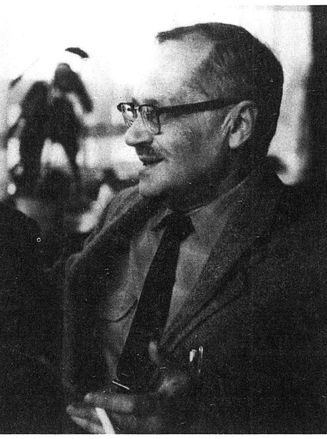
Jerzy Neyman, 1894-1981
How does one compute an interval estimate? How does one interpret an interval estimate? Can we make a probability statement about an interval estimate? How sure are we that the true value of the parameter lies within the interval?
In 1934, Jerzy Neyman presented a talk before the Royal Statistical Society, entitled “On the Two Different Aspects of the Representative Method.” His paper dealt with the analysis of sample surveys; it has the elegance of most of his work, deriving what appear to be simple mathematical expressions that are intuitively obvious (only after Neyman has derived them). The most important part of this paper is in an appendix, in which Neyman proposes a straightforward way to create an interval estimate and to determine how
accurate that estimate is. Neyman called this new procedure “confidence intervals,” and the ends of the confidence intervals he called “confidence bounds.”
Professor G. M. Bowley was in the chair for the meeting and rose to propose a vote of thanks. He first discussed the main part of the paper for several paragraphs. Then he got to the appendix:
I am not certain whether to ask for an explanation or to cast a doubt. It is suggested in the paper that the work is difficult to follow and I may be one of those who have been misled by it [later in this paragraph, he works out an example, showing that he clearly understood what Neyman was proposing]. I can only say that I have read it at the time it appeared and since, and I read Dr. Neyman’s elucidation of it yesterday with great care. I am referring to Dr. Neyman’s confidence limits. I am not at all sure that the “confidence” is not a “confidence trick.”
Bowley then works out an example of Neyman’s confidence interval and continues:
Does that really take us any further? Do we know more than was known to Todhunter [a late-nineteenth-century probabilist]? Does it take us beyond Karl Pearson and Edgeworth [a leading figure in the early development of mathematical statistics]? Does it really lead us towards what we need—the chance that in the universe which we are sampling the proportion is within these certain limits? I think it does not … . I do not know that I have expressed my thoughts quite accurately … [this] is a difficulty I have felt since the method was first propounded. The statement of the theory is not convincing, and until I am convinced I am doubtful of its validity.
Bowley’s problem with this procedure is one that has bedeviled the idea of confidence bounds since then. Clearly, the elegant four lines of calculus that Neyman used to derive his method are correct within the abstract mathematical theory of probability, and it does lead to the computation of a probability. However, it is not clear what that probability refers to. The data have been observed, the parameter is a fixed (if unknown) number, so the probability that the parameter takes on a specific value is either 100 percent if that was the value, or 0 if it was not. Yet, a 95 percent confidence interval deals with 95 percent probability. The probability of what? Neyman finessed this question by calling his creation a confidence interval and avoiding the use of the word probability. Bowley and others easily saw through this transparent ploy.
R. A. Fisher was also among the discussants, but he missed this point. His discussion was a rambling and confused collection of references to things that Neyman did not even include in his paper. This is because Fisher was in the midst of confusion over the calculation of interval estimates. In his comments, he referred to “fiducial probability,” a phrase that does not appear in Neyman’s paper. Fisher had long been struggling with this very problem—how to determine the degree of uncertainty associated with an interval estimate of a parameter. Fisher was working at the problem from a complicated angle somewhat related to his likelihood function. As he quickly proved, this way of looking at the formula did not meet the requirements of a probability distribution. Fisher called this function a “fiducial distribution,” but then he violated his own insights by applying the same mathematics one might apply to a proper probability distribution. The result, Fisher hoped, would be a set of values that was reasonable for the parameter, in the face of the observed data.
This was exactly what Neyman produced, and if the parameter was the mean of the normal distribution, both methods produced the same answers. From this, Fisher concluded that Neyman had stolen his idea of fiducial distribution and given it a different name.
Fisher never got far with his fiducial distributions, because the method broke down with other more complicated parameters, like the standard deviation. Neyman’s method works with any type of parameter. Fisher never appeared to understand the difference between the two approaches, insisting to the end of his life that Neyman’s confidence intervals were, at most, a generalization of his fiducial intervals. He was sure that Neyman’s apparent generalization would break down when faced with a sufficiently complicated problem—just as his own fiducial intervals had.
Neyman’s procedure does not break down, regardless of how complicated the problem, which is one reason it is so widely used in statistical analyses. Neyman’s real problem with confidence intervals was not the problem that Fisher anticipated. It was the problem that Bowley raised at the beginning of the discussion. What does probability mean in this context? In his answer, Neyman fell back on the frequentist definition of real-life probability. As he said here, and made clearer in a later paper on confidence intervals, the confidence interval has to be viewed not in terms of each conclusion but as a process. In the long run, the statistician who always computes 95 percent confidence intervals will find that the true value of the parameter lies within the computed interval 95 percent of the time. Note that, to Neyman, the probability associated with the confidence interval was not the probability that we are correct. It was the frequency of correct statements that a statistician who uses his method will make in the long run. It says nothing about how “accurate” the current estimate is.
As careful as Neyman was to define the concept, and as careful as were statisticians like Bowley to keep the concept of probability clear and uncontaminated, the general use of confidence intervals in science has led to much more sloppy thinking. It is not
uncommon, for instance, for someone using a 95 percent confidence interval to state that he is “95 percent sure” that the parameter lies within that interval. In chapter 13, we will meet L. J. (“Jimmie”) Savage and Bruno de Finetti and describe their work on personal probability, which justifies the use of statements like that. However, the calculation of the degree to which a person can be sure of something is different from the calculation of a confidence interval. The statistical literature has many articles where the bounds on a parameter that are derived following the methods of Savage and de Finetti are shown to be dramatically different from Neyman’s confidence bounds derived from the same data.
In spite of the questions about the meaning of probability in this context, Neyman’s confidence bounds have become the standard method of computing an interval estimate. Most scientists compute 90 percent or 95 percent confidence bounds and act as if they are sure that the interval contains the true value of the parameter.
No one talks or writes about “fiducial distributions” today. The idea died with Fisher. As he tried to make the idea work, Fisher produced a great deal of clever and important research. Some of that research has become mainstream; other parts remain in the incomplete state in which he left them.
In this research, Fisher came very close at times to stepping over the line into a branch of statistics he called “inverse probability.” Each time he pulled away. The idea of inverse probability began with the Reverend Thomas Bayes, an amateur mathematician of the eighteenth century. Bayes maintained a correspondence with many of the leading scientists of his age and often posed complicated mathematical problems to them. One day, while fiddling with the standard mathematical formulas of probability, he combined two of them with simple algebra and discovered Something that horrified him.
In the next chapter, we shall look at the Bayesian heresy and why Fisher refused to make use of inverse probability.