2
An Experiment to Challenge a Philosophy
We know that electrons have an electrical property: negative charge. Electrons also have a magnetic property called spin. In the first experimental observation of spin, a beam of silver atoms was aimed through a magnetic field that was stronger in some places than others.1 (We can create this kind of magnetic field by taking a horseshoe magnet and sharpening one of the poles.) If we send silver atoms between the poles of the magnet, we find that some atoms are deflected toward the north pole, and some are deflected toward the south pole (figure 1). No atoms pass straight through. Just like a coin toss, exactly two outcomes are possible.
This experiment is generally performed with neutral atoms—not isolated, negatively charged electrons. The deflection resulting from an electron’s charge overwhelms the deflection resulting from its spin. But the beauty of thought experiments is that we can ignore inconvenient details such as these. Let’s do a series of thought experiments in which the electron’s deflection results from its spin, and we ignore the deflection caused by its charge.

Figure 1 The arrows represent silver atoms passing through a magnetic field, with some deflecting toward the north pole (a), and some deflecting toward the south pole (b).
We imagine an experiment with special pairs of electrons. Suppose that the two electrons are emitted from a common source, and they travel in different directions. Each electron encounters a magnetic field. If the two magnets have the same alignment, the two electrons are always deflected in opposite directions: one to the north, and one to the south (figure 2). Because the behavior of one electron is linked so powerfully to the behavior of the other, we say the electrons are entangled.
In subsequent chapters, we’ll discuss experimental methods for creating pairs of entangled particles. In the laboratory, it’s easier to do experiments with entangled photons than with entangled electrons. For now, however, we’ll again set practical concerns aside.

Figure 2 A pair of entangled electrons with opposite magnetic properties: if the magnets are aligned, one electron must be deflected to the north pole, and one must be deflected to the south pole.
Imagine observing many pairs of entangled electrons passing through the magnetic fields. Half of the time, the electron on the left is deflected north and the electron on the right is deflected south. The other half of the time, the opposite occurs: the electron on the left is deflected south and the electron on the right is deflected north.
Here’s the key question: Does each electron have the magnetic property that is eventually observed (predisposition to northward or southward deflection) all along, or do the electrons “make up their minds” when they reach the magnets? In other words, does the measurement show us what the electrons were like all along, or does the measurement fundamentally change something? This may seem like a silly question, or at least one that cannot be empirically tested. What difference does it make whether the electrons were in the measured state all along, and what’s the big deal if they’re in an undecided state until the last minute? Indeed, I’ve been in an undecided state about what to order in a restaurant, and it’s only the “measurement” taken by the server that forces me to make up my mind.
This is the big deal: If the electrons make up their minds at the last minute, they must make opposite decisions. If one chooses northward deflection, the other must choose southward. How can they coordinate this, in defiance of locality, when they’re in different places? If the electrons make up their minds at the last minute and they always make opposite decisions, they’re like twins with a telepathic link, if you’ll forgive the analogy. This is “spooky action at a distance”—and Einstein argued strenuously against its existence.
To preserve locality (and avoid spooky action at a distance), we’d better hope for realism, which asserts that the electrons all along have the properties we end up measuring. In 1935, Einstein argued that quantum mechanics is an incomplete theory,2 like the probabilistic theories about quarters we considered in chapter 1. His argument is that the electrons are deflected in opposite directions because they were created with opposite magnetic properties. Quantum mechanics can’t tell us in advance which way each electron will be deflected; it can only tell us that each electron has a 50 percent chance of being deflected northward, and the other electron must be deflected southward (if the magnets are aligned).
To preserve locality (and avoid spooky action at a distance), we’d better hope for realism, which asserts that the electrons all along have the properties we end up measuring.
A complete theory should predict the magnetic property of each electron at the outset, if we believe that each electron has a definite magnetic property at the outset. We don’t know the details of this hypothetical, complete theory, and we don’t even know what factors predetermine the properties of the electrons. Since the unknown factors are hidden variables, the hypothetical, complete theory is a hidden variables theory. More specifically, we are interested in a local hidden variables theory: a theory that predicts the outcome of the measurement of a single electron, without any dependence on the other electron in the pair. A local hidden variables theory is thus an expression of the assumption of local realism.
For decades, physicists assumed that a local hidden variables theory could, in principle, complement quantum physics, filling in missing information and replacing probabilities with certainties. But the issue seemed academic or philosophical, and not subject to experiment: a local hidden variables theory determines the state of an electron before you measure it. Is it possible to measure the state an electron is in, before it’s measured? Seemingly it is not.
In 1964, John Bell made a stunning theoretical discovery, called Bell’s theorem.3 His original paper languished in obscurity for years, but enthusiasm for his discovery swelled over the course of decades. Bell showed that any local hidden variables theory imposes a constraint on measurable quantities. The constraint on measurable quantities is now called a Bell inequality. If the constraint is violated by measurement, then a local hidden variables theory cannot be valid. Moreover, because quantum physics predicts violations of the Bell inequality, quantum physics is fundamentally incompatible with any local hidden variables theory. So Einstein’s hope was in vain: a local hidden variables theory cannot complement quantum mechanics; it can only contradict it. And since measurable quantities determine whether a Bell inequality is violated or not, an experiment can be performed to determine whether the real world is consistent with quantum mechanics, or with a local hidden variables theory; we can’t have both. To reiterate these key points:
- • A Bell inequality is a constraint on a measurable quantity. An experiment can be done to test a Bell inequality. The experiment will either satisfy the Bell inequality or violate the Bell inequality.
- • If the experiment satisfies the Bell inequality, the experiment conforms to local realism but contradicts quantum physics.
- • If the experiment violates the Bell inequality, the experiment may conform to quantum physics but must contradict local realism.
Experimental results indeed violate Bell inequalities, thereby confirming quantum mechanics and overruling any possible local hidden variables theory. What does this mean? Either locality fails, or realism fails, or both fail: either one electron is influenced by the distant electron or the distant magnet, or the act of measurement creates a definite magnetic property that the electrons did not previously have, or both of these strange phenomena occur. (This is not a comprehensive list of interpretations of quantum mechanics, but it’s representative of possible consequences of rejecting local realism.)
Bell’s original theorem is too mathematical to prove in this book. Luckily, physicists have developed simplified versions of Bell’s theorem. We will see some of these in chapter 4, where we will prove that measured data contradict the philosophical assumption of local realism.
For now, we will investigate the fact that Bell established, without proving why it’s true. Bell asks us to imagine rotating the magnets encountered by the electron pairs. So, for example, we could rotate one magnet 180° relative to the other. If we do this, we find that the two electrons are always deflected toward the same pole: both to the north, or both to the south (figure 3).
Now we can imagine rotating the magnets to any angle, not just 180°. Let’s say a magnet is set to angle 0° if the south pole is directly above the north pole (like the magnets in figure 2). So the magnet is set to angle 180° if the north pole is directly above the south pole. We can do experiments in which either magnet is set to any angle.
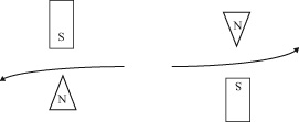
Figure 3 If one magnet is rotated 180° relative the other, the two electrons are always deflected toward the same pole: both north (as shown), or both south.
Bell asks us to think about just two numbers: +1 and −1. If the two electrons are deflected toward the same pole (both north or both south), we write down +1. If they’re deflected toward opposite poles (one north and one south), we write down −1. So, if the two magnets are aligned, the electrons are always deflected toward opposite poles (figure 2), and we always write −1. If one magnet is flipped 180° relative to the other, the two electrons are always deflected toward the same pole (figure 3), and we always write +1.
Bell asks us to think about three different magnet angles. Let’s choose 0°, 45°, and 90°. Then he asks us to do the following:
- • Set one magnet to 0° and one to 90°. Watch a bunch of electron pairs as they pass through the magnets. For each pair, write down +1 or −1 to indicate electron pairs deflected toward the same poles or opposite poles, respectively. Then, average all these numbers. Call this average number A.4 (Its value will be in the range of −1 to +1.)
- • Set one magnet to 45° and one to 90°. Again watch electron pairs as they pass through the magnets, and write down +1 or −1 for each pair. Average all these numbers. Call this average number B.
- • Set one magnet to 0° and one to 45°. Once again watch electron pairs as they pass through the magnets, and write down +1 or −1 for each pair. Average all these numbers. Call this average number C.
Now we have three numbers, A, B, and C, based on experimental measurements. Bell proved that the assumption of local realism requires
−1 − C ≤ A − B ≤ 1 + C.
That’s it! That’s the result of Bell’s theorem, the original Bell inequality. So, we now have a method to test a philosophical assumption. We simply perform measurements and calculate the three average numbers A, B, and C, as instructed above. Then we put these numbers in the Bell inequality. If the result is true, then we’ve satisfied the Bell inequality, and the data are consistent with the assumption of local realism. But if our data violate the Bell inequality, then we’ve contradicted local realism.
Let’s recall that local realism is an everyday assumption: observation merely reveals properties that an object already had, and the properties of an object are unaffected by the measurement of a distant object. This is the assumption that leads inexorably to the Bell inequality. The Bell inequality is, in fact, violated by measurement, so the assumption of local realism cannot be valid. We’ll explore the mysterious implications later in the book.
Next, we will look at the entanglement of light. Entangled light was used in the first experimental tests of Bell inequalities.