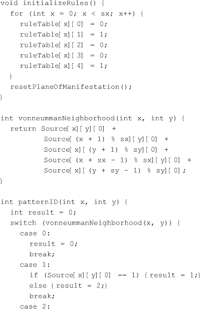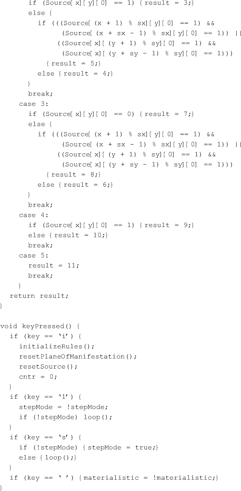

Here all the details of the computer algorithms used to generate Figures 12, 13, and 16 to 18 are shown. Initially, I thought of using symbolic mathematical notation to do this. However, ultimately I concluded that the computer code itself was a much less ambiguous, more direct and convenient alternative. Therefore, you will find below the code used to generate the figures.
The code has been written in “Processing,” an open source programming language and environment, based on Java, with special support for animations. At the time this book was written, Processing and its extensive documentation could be freely downloaded from http://www.processing.org. If you intend to run the programs below yourself, you will need to have Processing installed in your system. In what follows, I will assume that anyone interested in the level of detail in this appendix is relatively at ease with programming languages like Java.
The first program, shown below, is the one used to create a metaphor for the “Source,” as illustrated in Figures 12 and 13. It starts with some comments on how to use the program, as well as key variable declarations, which are also commented:


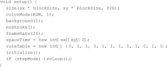
The next part of the code is the setup routine required by Processing. It defines the size of the window used to display the animation, the visual scheme used, and initializes some of the variables:
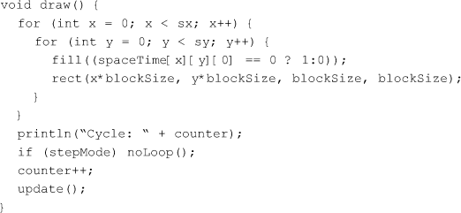
The next segment is the drawing function required by Processing, responsible for the main animation loop:
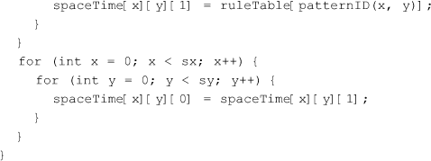
The function below is responsible for updating the states of the cellular automaton, carrying it over to the next generation:

To determine which of the twelve patterns illustrated in Figure 11 is present in a given neighborhood at a given iteration, it is convenient to, first, calculate the total number of live (black) cells in that neighborhood:

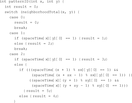
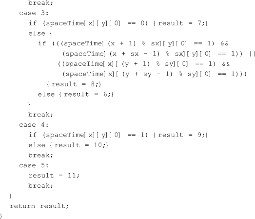
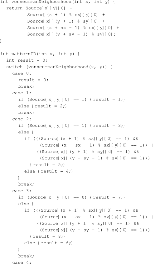
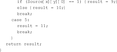
The function below can, then, actually identify which of those twelve patterns is at hand, using some computational shortcuts:
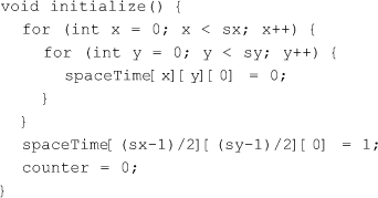
Here is some initialization code called early in the execution of the program. Notice that all cells are initialized to “dead” (white, or zero), while the center cell alone is initialized to “alive” (black, or one):
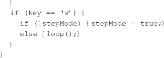
Finally, the code responsible for reading the user’s keyboard inputs to control the program:

The code for generating Figure 14 can be derived trivially from the program above. Therefore, it will not be discussed here.
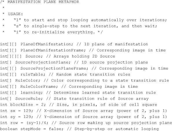
Now, below, you will find the complete code used to generate Figures 16 and 17. Keep in mind that this is an entirely separate, standalone program. Although the code for emulating the “Source” is repeated in it – since it is required for determining the “Source projection plane” – I will comment only on the new segments of the code, responsible for emulating the “plane of manifestation” and displaying the state transition rules with different shades of grey. Here is the beginning of the code where, once again, the variable declarations are commented so you can have an early idea about which variable represents what:

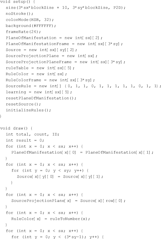
The setup and drawing routines below are analogous to what we have discussed earlier, except that several new variables now need to be initialized, and then recursively updated within the main drawing loop:
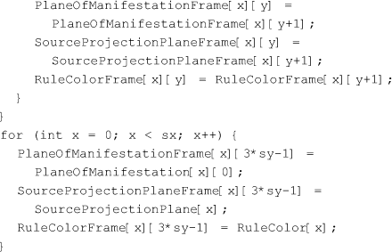
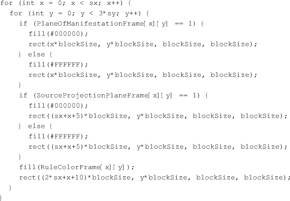
Here, the three columns of Figures 16 and 17 are actually drawn on the screen, after the corresponding variables have been updated above:
The next loop controls the transition of states in the 1D cellular automaton, corresponding to the “plane of manifestation,” onto its next generation:

In the lines below, the “vote” is performed across the three cells in a neighborhood within the plane of manifestation, to determine the next state of a cell. The cell’s own vote counts twice those of its two neighbors in the plane of manifestation. Notice that, when a tie occurs, the next state is determined directly by the Source projection plane:

Now, the cells must learn from the states that actually “manifest” after the vote. They learn not only from “direct experience,” but also from experiences “communicated” from their two neighbors in the plane of manifestation. Notice that learning from direct experience is twice as strong as learning from what is communicated from neighbors:

Now the Source is updated to its next generation:

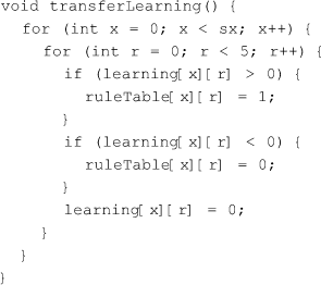
In the lines that follow, the resulting learning of the cells is transferred to their respective state transition rules, so the next generation of the automaton representing the plane of manifestation will be determined by these new, learned rules.
Below, the total amount of “live” cells in the cross-dimensional neighborhood shown in Figure 15 is counted, for the cellular automaton representing the plane of manifestation is a “totalistic cellular automaton;” that is, one that only considers the total amount of live cells in a neighborhood, not their specific configuration. This is done to simplify the metaphor and make its interpretation easier.

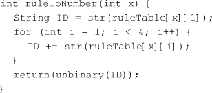
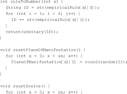
The routine below is used to convert a specific state transition rule into a single, unique number, so it can then be used to determine the shade of gray that is displayed in the rightmost column of Figures 16 and 17:
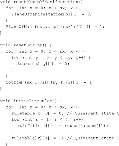
Now we have some reset and initialization functions to refresh the arrays. Notice that the plane of manifestation starts with a single “live” (black) cell in its center. Notice also that the state transition rule of each cell in the plane of manifestation is randomly, and independently, initialized:

The remaining code controls the unfolding of the Source Pattern, used to determine the contents of the “Source projection plane,” as already discussed earlier:
Finally, the minimalistic user interface code:

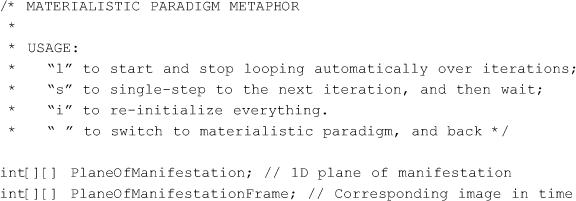
The third and last program, used to generate Figure 18, is shown below. It is very similar to the program already discussed above, so I will comment only on the segments that are different. Notice that, at some point, the user must push the space bar in order to trigger the transition to the “materialistic paradigm.”


In the function below, the state of the cell in the Source projection plane is only added, in calculating the corresponding neighborhood total, if the “materialistic paradigm” is not active. Otherwise, it is ignored, in a metaphor for the fact that the cells in the plane of manifestation no longer perceive the cross-dimensional influences from the Source.


The function below tracks the “apparent” state transition rules used in the plane of manifestation; that is, it represents an empirical model of the phenomena and circumstances observed in the plane of manifestation alone. Remember that the cellular automaton used is a totalistic one, so only the total number of “live” cells matters.

In the routine immediately below, each “apparent” state transition rule is converted into a unique number, representing a shade of gray, which is then displayed in the rightmost column of Figure 18.
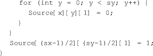
Unlike the previous program, this time the state transition rule of each cell in the plane of manifestation is initialized in the same way. This can be seen in the function immediately below. The idea is that we are no longer interested in the emergence of a single rule from a variety of randomly initialized ones, but solely in what happens at the moment of transition to a “materialistic paradigm” once the system has already converged to a uniform worldview.
