In science and engineering, we often encounter the problem of solving a system of linear equations. Matrices provide the most basic and useful mathematical tool for describing and solving such systems. As the introduction to matrix algebra, this chapter presents the basic operations and performance of matrices, followed by a description of vectorization of matrix and matricization of vector.
1.1 Basic Concepts of Vectors and Matrices
First we introduce the basic concepts and notation for vectors and matrices.
1.1.1 Vectors and Matrices


 , and
, and  . Here,
  (or
(or  ) denotes the set of real (or complex) numbers, and
  (or
(or  ) represents the set of all real (or complex) m-dimensional column vectors, while
  (or
(or  ) is the set of all m × n real (or complex) matrices.
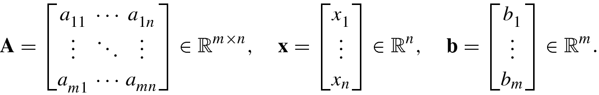
An m-dimensional row vector ![$$\mathbf {x}=[x_1^{\,} ,\ldots ,x_m ]$$](../images/492994_1_En_1_Chapter/492994_1_En_1_Chapter_TeX_IEq9.png) is represented as
is represented as  or
or  . To save writing space, an m-dimensional column vector is usually written as the transposed form of a row vector, denoted
 ![$$\mathbf {x}=[x_1^{\,} , \ldots ,x_m ]^T$$](../images/492994_1_En_1_Chapter/492994_1_En_1_Chapter_TeX_IEq12.png) , where T denotes “transpose.”
, where T denotes “transpose.”
Physical vector: Its elements are physical quantities with magnitude and direction, such as a displacement vector, a velocity vector, an acceleration vector, and so forth.
Geometric vector: A directed line segment or arrow can visualize a physical vector. Such a representation is known as a geometric vector. For example,
 represents the directed line segment with initial point A and terminal point B.
Algebraic vector: A geometric vector needs to be represented in algebraic form in order to operate. For a geometric vector
 on a plane, if its initial point is
  and its terminal point is
  , then the geometric vector
  can be represented in an algebraic form
  . Such a geometric vector described in algebraic form is known as an algebraic vector.
The vectors encountered often in practical applications are physical vectors, while geometric vectors and algebraic vectors are, respectively, the visual representation and the algebraic form of physical vectors. Algebraic vectors provide a computational tool for physical vectors.
Constant vector: All entries take real constant numbers or complex constant numbers, e.g., a = [1, 5, 2]T.
Function vector: Its entries take function values, e.g., x = [x 1, …, x n]T.
Random vector: It uses random variables or signals as entries, e.g.,
![$$\mathbf {x}(n)=[x_1^{\,} (n),\ldots ,x_m (n)]^T$$](../images/492994_1_En_1_Chapter/492994_1_En_1_Chapter_TeX_IEq19.png) where
where  are m random variables or signals.
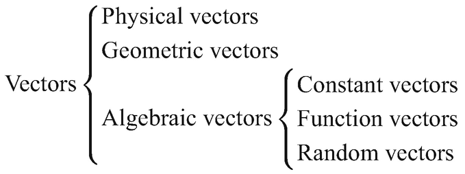
Classification of vectors
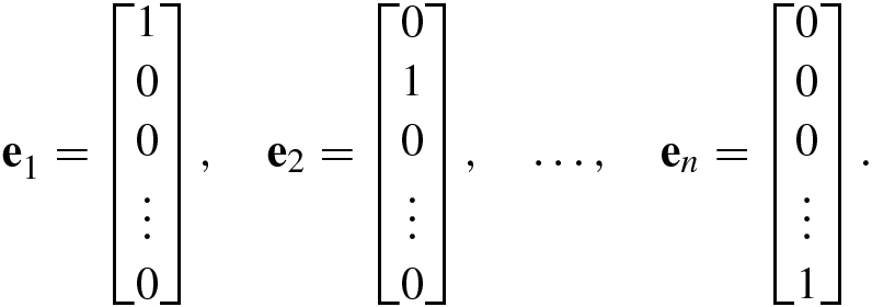
A vector all of whose components are equal to zero is called a zero vector and is denoted as 0 = [0, …, 0]T.
![$$\mathbf {x}=[x_1^{\,} ,\ldots ,x_n]^T$$](../images/492994_1_En_1_Chapter/492994_1_En_1_Chapter_TeX_IEq21.png) with only one nonzero entry x
i = 1 constitutes a basis vector, denoted e
i; e.g.,
with only one nonzero entry x
i = 1 constitutes a basis vector, denoted e
i; e.g.,
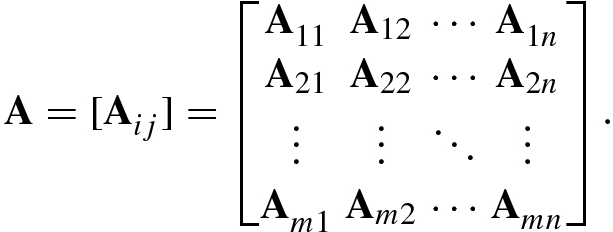
In modeling physical problems, the matrix A is usually the symbolic representation of a physical system (e.g., a linear system, a filter, or a learning machine).
An m × n matrix A is called a square matrix if m = n, a broad matrix for m < n, and a tall matrix for m > n.
The main diagonal of an n × n matrix A = [a ij] is the segment connecting the top left to the bottom right corner. The entries located on the main diagonal, a 11, a 22, …, a nn, are known as the (main) diagonal elements.


![$$\mathbf {I}= [{\mathbf {e}}_1^{\,} ,\ldots ,{\mathbf {e}}_n ]$$](../images/492994_1_En_1_Chapter/492994_1_En_1_Chapter_TeX_IEq22.png) using basis vectors.
using basis vectors.In this book, we use often the following matrix symbols.
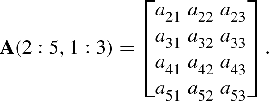
A(i, :) means the ith row of A.
A(:, j) means the jth column of A.
1.1.2 Basic Vector Calculus
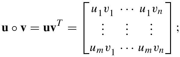
![$$\mathbf {u}=[u_1^{\,} ,\ldots ,u_n]^T$$](../images/492994_1_En_1_Chapter/492994_1_En_1_Chapter_TeX_IEq23.png) and
and ![$$\mathbf {v}=[v_1^{\,} ,\ldots ,v_n]^T$$](../images/492994_1_En_1_Chapter/492994_1_En_1_Chapter_TeX_IEq24.png) is defined as
is defined as
![$$\displaystyle \begin{aligned} \mathbf{u}+\mathbf{v}=[u_1^{\,} +v_1^{\,} ,\ldots ,u_n+v_n]^T. \end{aligned} $$](../images/492994_1_En_1_Chapter/492994_1_En_1_Chapter_TeX_Equ8.png)
Commutative law: u + v = v + u.
Associative law: (u + v) ±w = u + (v ±w) = (u ±w) + v.
![$$\displaystyle \begin{aligned} \alpha\mathbf{u}=[\alpha u_1^{\,} ,\ldots ,\alpha u_n]^T. \end{aligned} $$](../images/492994_1_En_1_Chapter/492994_1_En_1_Chapter_TeX_Equ9.png)

![$$\mathbf {u}=[u_1^{\,} ,\ldots ,u_n]^T$$](../images/492994_1_En_1_Chapter/492994_1_En_1_Chapter_TeX_IEq25.png) and
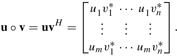
and ![$$\mathbf {v}=[v_1^{\,} ,\ldots ,v_n]^T$$](../images/492994_1_En_1_Chapter/492994_1_En_1_Chapter_TeX_IEq26.png) , their inner product (also called dot product or scalar product), denoted u ⋅v or 〈u, v〉, is defined as the real number
, their inner product (also called dot product or scalar product), denoted u ⋅v or 〈u, v〉, is defined as the real number


Note that if u and v are two row vectors, then u ⋅v = uv T for real vectors and u ⋅v = uv H for complex vectors.
1.1.3 Basic Matrix Calculus
![$$[{\mathbf {A}}^*]_{ij} =a_{ij}^*$$](../images/492994_1_En_1_Chapter/492994_1_En_1_Chapter_TeX_IEq27.png) , while the conjugate or Hermitian transpose of A, denoted
, while the conjugate or Hermitian transpose of A, denoted  , is defined as
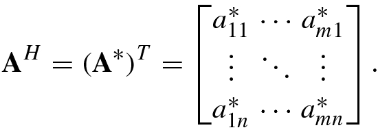
An n × n real (or complex) matrix satisfying A T = A (or A H = A) is called a symmetric matrix (or Hermitian matrix).

![$${\mathbf {A}}^H=[{\mathbf {A}}_{ji}^H]$$](../images/492994_1_En_1_Chapter/492994_1_En_1_Chapter_TeX_IEq29.png) is an n × m block matrix:
is an n × m block matrix: 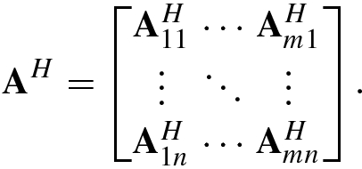
The simplest algebraic operations with matrices are the addition of two matrices and the multiplication of a matrix by a scalar.
Given two m × n matrices A = [a ij] and B = [b ij], matrix addition A + B is defined by [A + B]ij = a ij + b ij. Similarly, matrix subtraction A −B is defined as [A −B]ij = a ij − b ij.
Commutative law: A + B = B + A.
Associative law: (A + B) ±C = A + (B ±C) = (A ±C) + B.
![$$\displaystyle \begin{aligned}{}[\mathbf{AB}]_{ij} =\sum_{k=1}^n a_{ik} b_{kj},\quad i=1,\ldots ,m;~j=1,\ldots ,s. \end{aligned}$$](../images/492994_1_En_1_Chapter/492994_1_En_1_Chapter_TeX_Equd.png)
In particular, if B = αI, then [αA]ij = αa
ij. If ![$$\mathbf {B}=\mathbf {x}=[x_1^{\,} ,\ldots ,x_n ]^T$$](../images/492994_1_En_1_Chapter/492994_1_En_1_Chapter_TeX_IEq30.png) , then
, then ![$$[\mathbf {Ax}]_i =\sum _{j=1}^n a_{ij} x_j$$](../images/492994_1_En_1_Chapter/492994_1_En_1_Chapter_TeX_IEq31.png) for i = 1, …, m.
for i = 1, …, m.
- 1.
Associative law of multiplication: If
 , and
, and  , then A(BC) = (AB)C.
 - 2.
Left distributive law of multiplication: For two m × n matrices A and B, if C is an n × p matrix, then (A ±B)C = AC ±BC.
- 3.
Right distributive law of multiplication: If A is an m × n matrix, while B and C are two n × p matrices, then A(B ±C) = AB ±AC.
- 4.
If α is a scalar and A and B are two m × n matrices, then α(A + B) = αA + αB.
Note that the product of two matrices generally does not satisfy the commutative law, namely AB ≠ BA.
Another important operation on a square matrix is its inversion.
![$$\mathbf {x}=[x_1^{\,} ,\ldots ,x_n ]^T$$](../images/492994_1_En_1_Chapter/492994_1_En_1_Chapter_TeX_IEq34.png) and
and ![$$\mathbf {y}=[y_1^{\,} , \ldots ,y_n ]^T$$](../images/492994_1_En_1_Chapter/492994_1_En_1_Chapter_TeX_IEq35.png) . The matrix-vector product Ax = y can be regarded as a linear transform of the vector x, where the n × n matrix A is called the linear transform matrix. Let A
−1 denote the linear inverse transform of the vector y onto x. If A
−1 exists, then one has
. The matrix-vector product Ax = y can be regarded as a linear transform of the vector x, where the n × n matrix A is called the linear transform matrix. Let A
−1 denote the linear inverse transform of the vector y onto x. If A
−1 exists, then one has


Let A be an n × n matrix. The matrix A is said to be invertible if there is an n × n matrix A −1 such that AA −1 = A −1A = I, and A −1 is referred to as the inverse matrix of A.
- 1.The matrix conjugate, transpose, and conjugate transpose satisfy the distributive law:

- 2.The transpose, conjugate transpose, and inverse matrix of product of two matrices satisfy the following relationship:

in which both A and B are assumed to be invertible.
- 3.Each of the symbols for the conjugate, transpose, and conjugate transpose can be exchanged with the symbol for the inverse:

- 4.
For any m × n matrix A, both the n × n matrix B = A HA and the m × m matrix C = AA H are Hermitian matrices.
An n × n matrix A is nonsingular if and only if the matrix equation Ax = 0 has only the zero solution x = 0. If Ax = 0 exists for any nonzero solution x ≠ 0, then the matrix A is singular.
![$$\mathbf {A}=[{\mathbf {a}}_1^{\,} , \ldots ,{\mathbf {a}}_n ]$$](../images/492994_1_En_1_Chapter/492994_1_En_1_Chapter_TeX_IEq36.png) , the matrix equation Ax = 0 is equivalent to
, the matrix equation Ax = 0 is equivalent to 
its column vectors are linearly independent;
the matrix equation Ax = b exists a unique nonzero solution;
the matrix equation Ax = 0 has only a zero solution.
1.2 Sets and Linear Mapping
The set of all n-dimensional vectors with real (or complex) components is called a real (or complex) n-dimensional vector space, denoted  (or
(or  ). In real-world artificial intelligence problems, we are usually given N n-dimensional real data vectors
  that belong to a subset X other than the whole set
  . Such a subset is known as a vector subspace in n-dimensional vector space
  , denoted as
  . In this section, we present the sets, the vector subspaces, and the linear mapping of one vector subspace onto another.
1.2.1 Sets
As the name implies, a set is a collection of elements.
A set is usually denoted by S = {⋅}; inside the braces are the elements of the set S. If there are only a few elements in the set S, these elements are written out within the braces, e.g., S = {a, b, c}.
To describe the composition of a more complex set mathematically, the symbol “|” is used to mean “such that.” For example, S = {x|P(x) = 0} reads “the element x in set S such that P(x) = 0.” A set with only one element α is called a singleton, denoted {α}.
∀ denotes “for all ⋯”;
x ∈ A reads “x belongs to the set A”, i.e., x is an element or member of A;
x∉A means that x is not an element of the set A;
∋ denotes “such that”;
∃ denotes “there exists”;
 denotes “there does not exist”;
A ⇒ B reads “condition A results in B” or “A implies B.”

Let A and B be two sets; then the sets have the following basic relations.
The notation A ⊆ B reads “the set A is contained in the set B” or “A is a subset of B,” which implies that each element in A is an element in B, namely x ∈ A ⇒ x ∈ B.
If A ⊂ B, then A is called a proper subset of B. The notation B ⊃ A reads “B contains A” or “B is a superset of A.” The set with no elements is denoted by ∅ and is called the null set.
The notation A = B reads “the set A equals the set B,” which means that A ⊆ B and B ⊆ A, or x ∈ A ⇔x ∈ B (any element in A is an element in B, and vice versa). The negation of A = B is written as A ≠ B, implying that A does not belong to B, neither does B belong to A.


 denotes the set of nonzero vectors in complex n-dimensional vector space.


 denotes the Cartesian product of n sets
  , and its elements are the ordered n-ples
  :
:

1.2.2 Linear Mapping
Consider the transformation between vectors in two vector spaces. In mathematics, mapping is a synonym for mathematical function or for morphism.
A mapping T : V → W represents a rule for transforming the vectors in V to corresponding vectors in W. The subspace V is said to be the initial set or domain of the mapping T and W its final set or codomain.
When v is some vector in the vector space V , T(v) is referred to as the image of the vector v under the mapping T, or the value of the mapping T at the point v, whereas v is known as the original image of T(v).


 and all scalars
  .
.
If f(X, Y) is a scalar function with real matrices  and
and  as variables, then in linear mapping notation, the function can be denoted by the Cartesian product form
  .
.
 with high fidelity (Hi-Fi). By Hi-Fi, it means that there is the following linear relationship between any input signal vector u and the corresponding output signal vector Au of the amplifier:
T : V → W is a one-to-one mapping if it is either injective mapping or surjective mapping, i.e., T(x) = T(y) implies x = y or distinct elements have distinct images.
A one-to-one mapping T : V → W has an inverse mapping T −1 : W → V . The inverse mapping T −1 restores what the mapping T has done. Hence, if T(v) = w, then T −1(w) = v, resulting in T −1(T(v)) = v, ∀ v ∈ V and T(T −1(w)) = w, ∀ w ∈ W.
If  are the input vectors of a system T in engineering, then
  T(u
p) can be viewed as the output vectors of the system. The criterion for identifying whether a system is linear is: if the system input is the linear expression
T(u
p) can be viewed as the output vectors of the system. The criterion for identifying whether a system is linear is: if the system input is the linear expression  , then the system is said to be linear only if its output satisfies the linear expression
  . Otherwise, the system is nonlinear.
The following are intrinsic relationships between a linear space and a linear mapping.
if M is a linear subspace in V , then T(M) is a linear subspace in W;
if N is a linear subspace in W, then the linear inverse transform T −1(N) is a linear subspace in V .
For a given linear transformation y = Ax, if our task is to obtain the output vector y from the input vector x given a transformation matrix A, then Ax = y is said to be a forward problem. Conversely, the problem of finding the input vector x from the output vector y is known as an inverse problem. Clearly, the essence of the forward problem is a matrix-vector calculation, while the essence of the inverse problem is to solve a matrix equation.
1.3 Norms
Many problems in artificial intelligence need to solve optimization problems in which vector and/or matrix norms are the cost function terms to be optimized.
1.3.1 Vector Norms
 is called the vector norm of x ∈ V , if for all vectors x, y ∈ V and any scalar
  (here
(here  denotes
  or
or  ), the following three norm axioms hold:
Nonnegativity: p(x) ≥ 0 and p(x) = 0 ⇔x = 0.
Homogeneity: p(cx) = |c|⋅ p(x) is true for all complex constant c.
Triangle inequality: p(x + y) ≤ p(x) + p(y).
- 1.
∥0∥ = 0 and ∥x∥ > 0, ∀ x ≠ 0.
- 2.
∥cx∥ = |c| ∥x∥ holds for all vector x ∈ V and any scalar
 .
. - 3.Polarization identity: For real inner product spaces we have
 (1.3.1)and for complex inner product spaces we have
 (1.3.2)
 - 4.Parallelogram law
 (1.3.3)
 - 5.Triangle inequality
 (1.3.4)
 - 6.Cauchy–Schwartz inequality
 (1.3.5)
The equality |〈x, y〉| = ∥x∥⋅∥y∥ holds if and only if y = c x, where c is some nonzero complex constant.
- ℓ 0-normThat is,

 (1.3.6)
  -norm
i.e., ∥x∥1 is the sum of absolute (or modulus) values of nonzero entries of x.
-norm
i.e., ∥x∥1 is the sum of absolute (or modulus) values of nonzero entries of x. (1.3.7)
 -norm or the Euclidean norm
 (1.3.8)
 -norm
-norm
 (1.3.9)


The ℓ 0-norm does not satisfy the homogeneity ∥cx∥0 = |c|⋅∥x∥0, and thus is a quasi-norm, while the ℓ p-norm is also a quasi-norm if 0 < p < 1 but a norm if p ≥ 1.
Clearly, when p = 1 or p = 2, the ℓ p-norm reduces to the ℓ 1-norm or the ℓ 2-norm, respectively.


- Measuring the size or length of a vector:which is called the Euclidean length.
 (1.3.13)
 - Defining the 𝜖-neighborhood of a vector x:
 (1.3.14)
 - Measuring the distance between vectors x and y:This is known as the Euclidean distance.
 (1.3.15)
 - Defining the angle θ (0 ≤ θ ≤ 2π) between vectors x and y:
 (1.3.16)
A vector with unit Euclidean length is known as a normalized (or standardized) vector. For any nonzero vector  , x∕〈x, x〉1∕2 is the normalized version of the vector and has the same direction as x.
The norm ∥x∥ is said to be a unitary invariant norm if ∥Ux∥ = ∥x∥ holds for all vectors  and all unitary matrices
  such that U
HU = I.
such that U
HU = I.
The Euclidean norm ∥⋅∥2 is unitary invariant.
If the inner product 〈x, y〉 = x Hy = 0, then the angle between the vectors θ = π∕2, from which we have the following definition on orthogonality of two vectors.
Two constant vectors x and y are said to be orthogonal, denoted by x ⊥ y, if their inner product 〈x, y〉 = x Hy = 0.
 , and let the definition field of the function variable t be [a, b] with a < b. Then the inner product of the function vectors x(t) and y(t) is defined as


The following proposition shows that, for any two orthogonal vectors, the square of the norm of their sum is equal to the sum of the squares of the respective vector norms.
If x ⊥ y, then ∥x + y∥2 = ∥x∥2 + ∥y∥2.


This proposition is also referred to as the Pythagorean theorem.
Mathematical definitions: Two vectors x and y are orthogonal if their inner product is equal to zero, i.e., 〈x, y〉 = 0.
Geometric interpretation: If two vectors are orthogonal, then their angle is π∕2, and the projection of one vector onto the other vector is equal to zero.
Physical significance: When two vectors are orthogonal, each vector contains no components of the other, that is, there exist no interactions or interference between these vectors.
1.3.2 Matrix Norms
The inner product and norms of vectors can be easily extended to the inner product and norms of matrices.
![$$\mathbf {A}=[{\mathbf {a}}_1^{\,} ,\ldots ,{\mathbf {a}}_n ]$$](../images/492994_1_En_1_Chapter/492994_1_En_1_Chapter_TeX_IEq73.png) and
and ![$$\mathbf {B}=[{\mathbf {b}}_1^{\,} ,\ldots ,{\mathbf {b}}_n ]$$](../images/492994_1_En_1_Chapter/492994_1_En_1_Chapter_TeX_IEq74.png) , stack them, respectively, into the following mn × 1 vectors according to their columns:
, stack them, respectively, into the following mn × 1 vectors according to their columns: 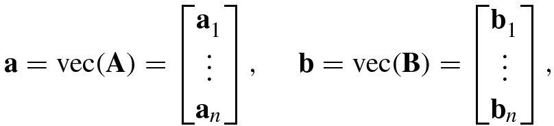
 , is defined as the inner product of two elongated vectors:


- 1.
 -norm (p = 1)
 (1.3.24)
 - 2.Frobenius norm (p = 2)
 (1.3.25)
is the most common matrix norm. Clearly, the Frobenius norm is an extension of the Euclidean norm of the vector to the elongated vector a = [a 11, …, a m1, …, a 1n, …, a mn]T.
- 3.Max norm or ℓ ∞-norm (p = ∞)
 (1.3.26)

 and
and  are the maximum eigenvalue of A
HA and the maximum singular value of A, respectively.
are the maximum eigenvalue of A
HA and the maximum singular value of A, respectively. , the Frobenius norm can be also written in the form of the trace function as follows:
 is the rank of A. Clearly, we have

- Cauchy–Schwartz inequlityThe equals sign holds if and only if A = c B, where c is a complex constant.
 (1.3.31)
 - Pythagoras’ theorem
 (1.3.32)
 - Polarization identity
 (1.3.33)where
 (1.3.34)
 represents the real part of the inner product 〈A, B〉.
1.4 Random Vectors
In science and engineering applications, the measured data are usually random variables. A vector with random variables as its entries is called a random vector.
In this section, we discuss the statistics and properties of random vectors by focusing on Gaussian random vectors.
1.4.1 Statistical Interpretation of Random Vectors
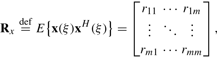
In the statistical interpretation of random vectors, the first-order and second-order statistics of random vectors are the most important.

![$$E\{\mathbf {x}(\xi )\}=[E\{x_1^{\,} (\xi )\},\ldots ,E\{x_n^{\,} (\xi )\}]^T$$](../images/492994_1_En_1_Chapter/492994_1_En_1_Chapter_TeX_IEq82.png) and the function variable ξ may be time t, circular frequency f, angular frequency ω or space parameter s, and so on.
and the function variable ξ may be time t, circular frequency f, angular frequency ω or space parameter s, and so on.
![$$\mathbf {x}(\xi )=[x_1^{\,} (\xi ),\ldots ,x_m (\xi )]^T$$](../images/492994_1_En_1_Chapter/492994_1_En_1_Chapter_TeX_IEq83.png) , its mean vector μ
x is defined as
, its mean vector μ
x is defined as 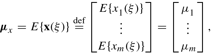


 of the random variable x
i(ξ), whereas the other entries
of the random variable x
i(ξ), whereas the other entries ![$$\displaystyle \begin{aligned} c_{ij} \stackrel{\mathrm{def}}{=}E\big\{ [x_i (\xi )-\mu_i ][x_j (\xi )-\mu_j ]^*\big\}=E\big\{ x_i (\xi )x_j^* (\xi ) \big\} -\mu_i \mu_j^* =c_{ji}^* \end{aligned} $$](../images/492994_1_En_1_Chapter/492994_1_En_1_Chapter_TeX_Equ74.png)

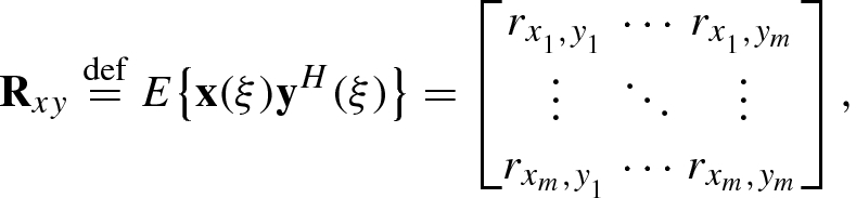
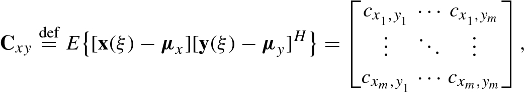
 is the cross-correlation of the random vectors x
i(ξ) and y
j(ξ) and
is the cross-correlation of the random vectors x
i(ξ) and y
j(ξ) and ![$$c_{x_i ,y_j} \stackrel {\mathrm {def}}{=}E\{ [x_i (\xi )-\mu _{x_i} ][y_j (\xi )-\mu _{y_j}]^*\}$$](../images/492994_1_En_1_Chapter/492994_1_En_1_Chapter_TeX_IEq86.png) is the cross-covariance of x
i(ξ) and y
j(ξ).
is the cross-covariance of x
i(ξ) and y
j(ξ).
![$$\displaystyle \begin{aligned} \mathbf{x}\leftarrow \mathbf{x}=[x(0)-\mu_x ,x(1)-\mu_x ,\ldots ,x(N-1)-\mu_x ]^T, \end{aligned}$$](../images/492994_1_En_1_Chapter/492994_1_En_1_Chapter_TeX_Equq.png)
 .
.After zero-mean normalization, the correlation matrices and covariance matrices are equal, i.e., R x = C x and R xy = C xy.
- 1.
The autocorrelation matrix is Hermitian, i.e.,
 .
. - 2.
The autocorrelation matrix of the linear combination vector y = Ax + b satisfies R y = AR xA H.
- 3.
The cross-correlation matrix is not Hermitian but satisfies
 .
. - 4.
 .
. - 5.
If x and y have the same dimension, then R x+y = R x + R xy + R yx + R y.
- 6.
R Ax,By = AR xyB H.

 is the cross-covariance of the random variables x(ξ) and y(ξ), while
  and
and  are, respectively, the variances of x(ξ) and y(ξ). Applying the Cauchy–Schwartz inequality to Eq. (1.4.15), we have
The closer ρ xy is to zero, the weaker the similarity of the random variables x(ξ) and y(ξ) is.
The closer ρ xy is to 1, the more similar x(ξ) and y(ξ) are.
The case ρ xy = 0 means that there are no correlated components between the random variables x(ξ) and y(ξ). Thus, if ρ xy = 0, the random variables x(ξ) and y(ξ) are said to be uncorrelated. Since this uncorrelation is defined in a statistical sense, it is usually said to be a statistical uncorrelation.
It is easy to verify that if x(ξ) = c y(ξ), where c is a complex number, then |ρ xy| = 1. Up to a fixed amplitude scaling factor |c| and a phase ϕ(c), the random variables x(ξ) and y(ξ) are the same, so that x(ξ) = c ⋅ y(ξ) = |c|ejϕ(c)y(ξ). Hence, if |ρ xy| = 1, then random variables x(ξ) and y(ξ) are said to be completely correlated or coherent.
Two random vectors  and
and 
![$$\ldots ,y_n^{\,} (\xi )]^T$$](../images/492994_1_En_1_Chapter/492994_1_En_1_Chapter_TeX_IEq96.png) are said to be statistically uncorrelated if their cross-covariance matrix C
xy = O
m×n or, equivalently,
are said to be statistically uncorrelated if their cross-covariance matrix C
xy = O
m×n or, equivalently,  .
.


Note that for the zero-mean normalized m × 1 random vector x(ξ) and n × 1 normalized random vector y(ξ), their statistical uncorrelation and orthogonality are equivalent, as their cross-covariance and cross-correlation matrices are equal, i.e., C xy = R xy.
1.4.2 Gaussian Random Vectors
If each entry x
i(ξ), i = 1, …, m, is Gaussian random variable, then the random vector ![$$\mathbf {x}=[x_1^{\,} (\xi ),\ldots ,x_m (\xi )]^T$$](../images/492994_1_En_1_Chapter/492994_1_En_1_Chapter_TeX_IEq98.png) is called a Gaussian random vector.
is called a Gaussian random vector.
Let  denote a real Gaussian or normal random vector with the mean vector
 ![$$\bar {\mathbf {x}}=[\bar x_1^{\,} ,\ldots ,\bar x_m ]^T$$](../images/492994_1_En_1_Chapter/492994_1_En_1_Chapter_TeX_IEq100.png) and covariance matrix
and covariance matrix  . If each entry of the Gaussian random vector is independent identically distributed (iid), then its covariance matrix
  , where
  is the variance of the Gaussian random variable x
i.
is the variance of the Gaussian random variable x
i.
 is the joint probability density function of its m random variables, i.e.,

 is also given by Eq. (1.4.19), but the exponential term becomes [25, 29]
 ![$$\displaystyle \begin{aligned} (\mathbf{x}-\bar{\mathbf{x}})^T{\boldsymbol \Gamma}_x^{-1}(\mathbf{x}-\bar{\mathbf{x}})=\sum_{i=1}^m\sum_{j=1}^m [{\boldsymbol \Gamma}_x^{-1}]_{i,j} (x_i -\mu_i ) (x_j -\mu_j ), \end{aligned} $$](../images/492994_1_En_1_Chapter/492994_1_En_1_Chapter_TeX_Equ84.png)
![$$[{\boldsymbol \Gamma }_x^{-1}]_{ij}$$](../images/492994_1_En_1_Chapter/492994_1_En_1_Chapter_TeX_IEq106.png) represents the (i, j)th entry of the inverse matrix
represents the (i, j)th entry of the inverse matrix  and μ
i = E{x
i} is the mean of the random variable x
i.
and μ
i = E{x
i} is the mean of the random variable x
i.
![$${\boldsymbol \omega }=[\omega _1^{\,} ,\ldots ,\omega _m]^T$$](../images/492994_1_En_1_Chapter/492994_1_En_1_Chapter_TeX_IEq108.png) .
. , then
 ![$$\mathbf {x}=[x_1^{\,} ,\ldots ,x_m ]^T$$](../images/492994_1_En_1_Chapter/492994_1_En_1_Chapter_TeX_IEq110.png) is called a complex Gaussian random vector, denoted x ∼ CN(μ
x, Γ
x), where
is called a complex Gaussian random vector, denoted x ∼ CN(μ
x, Γ
x), where ![$${\boldsymbol \mu }_x =[\mu _1^{\,} ,\ldots ,\mu _m ]^T$$](../images/492994_1_En_1_Chapter/492994_1_En_1_Chapter_TeX_IEq111.png) and Γ are, respectively, the mean vector and the covariance matrix of the random vector x. If x
i = u
i + jv
i and the random vectors
and Γ are, respectively, the mean vector and the covariance matrix of the random vector x. If x
i = u
i + jv
i and the random vectors ![$$[u_1^{\,} ,v_1^{\,} ]^T,\ldots ,[u_m ,v_m ]^T$$](../images/492994_1_En_1_Chapter/492994_1_En_1_Chapter_TeX_IEq112.png) are statistically independent of each other, then the probability density function of a complex Gaussian random vector x is given by Poularikas [29, p. 35-5]
are statistically independent of each other, then the probability density function of a complex Gaussian random vector x is given by Poularikas [29, p. 35-5]

 . The characteristic function of the complex Gaussian random vector x is determined by
The probability density function of x is completely described by its mean vector and covariance matrix.
If two Gaussian random vectors x and y are statistically uncorrelated, then they are also statistically independent.
- Given a Gaussian random vector x with mean vector μ x and covariance matrix Γ x, the random vector y obtained by the linear transformation y(ξ) = Ax(ξ) is also a Gaussian random vector, and its probability density function is given byfor real Gaussian random vectors and
 (1.4.24)for complex Gaussian random vectors.
 (1.4.25)

 x
m(t)]T. If x
i(t), i = 1, …, m, have zero mean and the same variance σ
2, then the real part x
R,i(t) and the imaginary part x
I,i(t) are two real white Gaussian noises that are statistically independent and have the same variance. This implies that
x
m(t)]T. If x
i(t), i = 1, …, m, have zero mean and the same variance σ
2, then the real part x
R,i(t) and the imaginary part x
I,i(t) are two real white Gaussian noises that are statistically independent and have the same variance. This implies that 

 are statistically uncorrelated, we have

1.5 Basic Performance of Matrices
For a multivariate representation with mn components, we need some scalars to describe the basic performance of an m × n matrix.
1.5.1 Quadratic Forms
The quadratic form of an n × n matrix A is defined as x HAx, where x may be any n × 1 nonzero vector. In order to ensure the uniqueness of the definition of quadratic form (x HAx)H = x HAx, the matrix A is required to be Hermitian or complex conjugate symmetric, i.e., A H = A. This assumption ensures also that any quadratic form function is real-valued. One of the basic advantages of a real-valued function is its suitability for comparison with a zero value.
Quadratic forms and positive definiteness of a Hermitian matrix A
Quadratic forms | Symbols | Positive definiteness |
|---|---|---|
x HAx > 0 | A ≻ 0 | A is a positive definite matrix |
x HAx ≥ 0 | A ≽ 0 | A is a positive semi-definite matrix |
x HAx < 0 | A ≺ 0 | A is a negative definite matrix |
x HAx ≤ 0 | A ≼ 0 | A is a negative semi-definite matrix |
A Hermitian matrix A is said to be indefinite matrix if x HAx > 0 for some nonzero vectors x and x HAx < 0 for other nonzero vectors x.
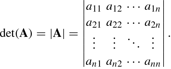
1.5.2 Determinants
 or |A|, is defined as
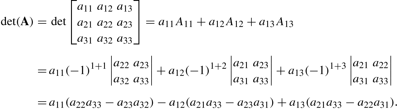
 of the remaining matrix A
ij is known as the cofactor of the entry a
ij. In particular, when j = i, A
ii is known as the principal minor of A. The cofactor A
ij is related to the determinant of the submatrix A
ij as follows:
of the remaining matrix A
ij is known as the cofactor of the entry a
ij. In particular, when j = i, A
ii is known as the principal minor of A. The cofactor A
ij is related to the determinant of the submatrix A
ij as follows:


A matrix with nonzero determinant is known as a nonsingular matrix.
- 1.
If two rows (or columns) of a matrix A are exchanged, then the value of
 remains unchanged, but the sign is changed.
 - 2.
If some row (or column) of a matrix A is a linear combination of other rows (or columns), then
 . In particular, if some row (or column) is proportional or equal to another row (or column), or there is a zero row (or column), then
  .
. - 3.
The determinant of an identity matrix is equal to 1, i.e.,
 .
. - 4.
Any square matrix A and its transposed matrix A T have the same determinant, i.e.,
 ; however,
  .
. - 5.The determinant of a Hermitian matrix is real-valued, since
 (1.5.5)
 - 6.The determinant of the product of two square matrices is equal to the product of their determinants, i.e.,
 (1.5.6)
 - 7.
For any constant c and any n × n matrix A,
 .
. - 8.
If A is nonsingular, then
 .
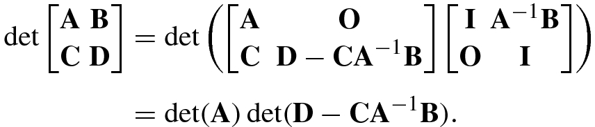
. - 9.For matrices A m×m, B m×n, C n×m, D n×n, the determinant of the block matrix for nonsingular A is given by
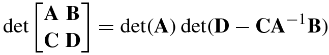 (1.5.7)and for nonsingular D we have
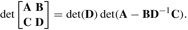 (1.5.8)
 - 10.The determinant of a triangular (upper or lower triangular) matrix A is equal to the product of its main diagonal entries:

The determinant of a diagonal matrix A = Diag(a 11, …, a nn) is also equal to the product of its diagonal entries.
The determinant of a positive definite matrix A is larger than 0, i.e.,
 .
.The determinant of a positive semi-definite matrix A is larger than or equal to 0, i.e.,
 .
.
1.5.3 Matrix Eigenvalues


If (1.5.11) holds for λ = 0, then
 . This implies that as long as a matrix A has a zero eigenvalue, this matrix must be singular.
All the eigenvalues of a zero matrix are zero, and for any singular matrix there exists at least one zero eigenvalue. Clearly, if all n diagonal entries of an n × n singular matrix A contain a subtraction of the same scalar x ≠ 0 that is not an eigenvalue of A then the matrix A − xI must be nonsingular, since |A − xI|≠ 0.
- 1.For A m×m and B m×m, eig(AB) = eig(BA) because

where u′ = Bu. However, if the eigenvector of AB corresponding to λ is u, then the eigenvector of BA corresponding to the same λ is u′ = Bu.
- 2.
If rank(A) = r, then the matrix A has at most r different eigenvalues.
- 3.
The eigenvalues of the inverse matrix satisfy eig(A −1) = 1∕eig(A).
- 4.Let I be the identity matrix; then
 (1.5.12)
 (1.5.13)
Positive definite matrix: Its all eigenvalues are positive real numbers.
Positive semi-definite matrix: Its all eigenvalues are nonnegative.
Negative definite matrix: Its all eigenvalues are negative.
Negative semi-definite matrix: Its all eigenvalues are nonpositive.
Indefinite matrix: It has both positive and negative eigenvalues.

Method for improving the numerical stability: Consider the matrix equation Ax = b, where A is usually positive definite or nonsingular. However, owing to noise or errors, A may sometimes be close to singular. We can alleviate this difficulty as follows. If λ is a small positive number, then − λ cannot be an eigenvalue of A. This implies that the characteristic equation |A − xI| = |A − (−λ)I| = |A + λI| = 0 cannot hold for any λ > 0, and thus the matrix A + λI must be nonsingular. Therefore, if we solve (A + λI)x = b instead of the original matrix equation Ax = b, and λ takes a very small positive value, then we can overcome the singularity of A to improve greatly the numerical stability of solving Ax = b. This method for solving (A + λI)x = b, with λ > 0, instead of Ax = b is the well-known Tikhonov regularization method for solving nearly singular matrix equations.
Method for improving the accuracy: For a matrix equation Ax = b, with the data matrix A nonsingular but containing additive interference or observation noise, if we choose a very small positive scalar λ to solve (A − λI)x = b instead of Ax = b, then the influence of the noise of the data matrix A on the solution vector x will be greatly decreased. This is the basis of the well-known total least squares (TLS) method.
1.5.4 Matrix Trace

Clearly, for a random signal x = [x
1, …, x
n]T, the trace of its autocorrelation matrix R
x,  , denotes the energy of the random signal.
The following are some properties of the matrix trace.
- 1.
If both A and B are n × n matrices, then tr(A ±B) = tr(A) ±tr(B).
- 2.
If A and B are n × n matrices and
 and c
2 are constants, then
and c
2 are constants, then  . In particular, tr(cA) = c ⋅tr(A).
 - 3.
tr(A T) = tr(A), tr(A ∗) = (tr(A))∗ and tr(A H) = (tr(A))∗.
- 4.
If
 , then tr(AB) = tr(BA).
 - 5.
If A is an m × n matrix, then tr(A HA) = 0 implies that A is an m × n zero matrix.
- 6.
x HAx = tr(Axx H) and y Hx = tr(xy H).
- 7.
The trace of an n × n matrix is equal to the sum of its eigenvalues, namely
 .
. - 8.The trace of a block matrix satisfies
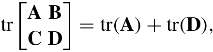
where
 and
and  .
. - 9.For any positive integer k, we have
 (1.5.16)


1.5.5 Matrix Rank
Among a set of p-dimensional (row or column) vectors, there are at most p linearly independent (row or column) vectors.
For an m × n matrix A, the number of linearly independent rows and the number of linearly independent columns are the same.
From this theorem we have the following definition of the rank of a matrix.
The rank of an m × n matrix A is defined as the number of its linearly independent rows or columns.
It needs to be pointed out that the matrix rank gives only the number of linearly independent rows or columns, but it gives no information on the locations of these independent rows or columns.
If
 , then A is known as a rank-deficient matrix.
If rank(A m×n) = m (< n), then the matrix A is a full row rank matrix.
If rank(A m×n) = n (< m), then the matrix A is called a full column rank matrix.
If rank(A n×n) = n, then A is said to be a full-rank matrix (or nonsingular matrix).
The matrix equation A m×nx n×1 = b m×1 is said to be a consistent equation, if it has at least one exact solution. A matrix equation with no exact solution is said to be an inconsistent equation.
A matrix A with  has
has  linearly independent column vectors. All linear combinations of the
  linearly independent column vectors constitute a vector space, called the column space or the range or the manifold of A.
The column space Col(A) = Col(a
1, …, a
n) or the range Range(A) = Range(a
1, …, a
n) is  -dimensional. Hence the rank of a matrix can be defined by using the dimension of its column space or range, as described below.

rank(A) = k;
there are k and not more than k columns (or rows) of A that combine a linearly independent set;
there is a k × k submatrix of A with nonzero determinant, but all the (k + 1) × (k + 1) submatrices of A have zero determinant;
the dimension of the column space Col(A) or the range Range(A) equals k;
k = n −dim[Null(A)], where Null(A) denotes the null space of the matrix A.

If premultiplying an m × n matrix A by an m × m nonsingular matrix P, or postmultiplying it by an n × n nonsingular matrix Q, then the rank of A is not changed, namely rank(PAQ) = rank(A).
The rank is a positive integer.
The rank is equal to or less than the number of columns or rows of the matrix.
Premultiplying any matrix A by a full column rank matrix or postmultiplying it by a full row rank matrix, then the rank of the matrix A remains unchanged.
- 1.
If
 , then rank(A
H) = rank(A
T) = rank(A
∗) = rank(A).
, then rank(A
H) = rank(A
T) = rank(A
∗) = rank(A). - 2.
If
 and c ≠ 0, then rank(cA) = rank(A).
 - 3.If
 , and
, and  are nonsingular, then
That is, after premultiplying and/or postmultiplying by a nonsingular matrix, the rank of B remains unchanged.
- 4.
For
 , rank(A) = rank(B) if and only if there exist nonsingular matrices
  and
and  such that B = XAY.
 - 5.
rank(AA H) = rank(A HA) = rank(A).
- 6.
If
 , then
  is nonsingular.
The commonly used rank inequalities is  for any m × n matrix A.
1.6 Inverse Matrices and Moore–Penrose Inverse Matrices
Matrix inversion is an important aspect of matrix calculus. In particular, the matrix inversion lemma is often used in science and engineering. In this section we discuss the inverse of a full-rank square matrix, the pseudo-inverse of a non-square matrix with full row (or full column) rank, and the inversion of a rank-deficient matrix.
1.6.1 Inverse Matrices
A nonsingular matrix A is said to be invertible, if its inverse A −1 exists so that A −1A = AA −1 = I.
A is nonsingular.
A −1 exists.
rank(A) = n.
All rows of A are linearly independent.
All columns of A are linearly independent.
 .
.The dimension of the range of A is n.
The dimension of the null space of A is equal to zero.
Ax = b is a consistent equation for every
 .
.Ax = b has a unique solution for every b.
Ax = 0 has only the trivial solution x = 0.
- 1.
A −1A = AA −1 = I.
- 2.
A −1 is unique.
- 3.
The determinant of the inverse matrix is equal to the reciprocal of the determinant of the original matrix, i.e., |A −1| = 1∕|A|.
- 4.
The inverse matrix A −1 is nonsingular.
- 5.
The inverse matrix of an inverse matrix is the original matrix, i.e., (A −1)−1 = A.
- 6.
The inverse matrix of a Hermitian matrix A = A H satisfies (A H)−1 = (A −1)H = A −1. That is to say, the inverse matrix of any Hermitian matrix is a Hermitian matrix as well.
- 7.
(A ∗)−1 = (A −1)∗.
- 8.
If A and B are invertible, then (AB)−1 = B −1A −1.
- 9.If
 is a diagonal matrix, then its inverse matrix
- 10.
Let A be nonsingular. If A is an orthogonal matrix, then A −1 = A T, and if A is a unitary matrix, then A −1 = A H.

Lemma 1.2 is called the matrix inversion lemma, and was presented by Sherman and Morrison [37] in 1950.


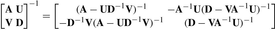
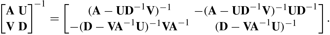
The following are inversion formulas for block matrices.

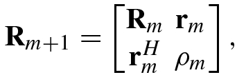
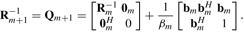
 using
using  , let
, let 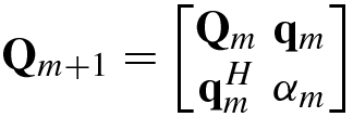
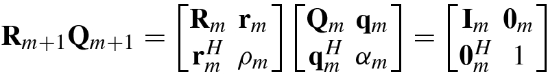


![$$\displaystyle \begin{aligned} {\mathbf{b}}_m &\stackrel{\mathrm{def}}{=}[ b_0^{(m)},b_1^{(m)} ,\ldots ,b_{m-1}^{(m)}]^T=-{\mathbf{R}}_m^{-1} {\mathbf{r}}_m, \end{aligned} $$](../images/492994_1_En_1_Chapter/492994_1_En_1_Chapter_TeX_Equ138.png)


1.6.2 Left and Right Pseudo-Inverse Matrices
From a broader perspective, any n × m matrix G may be called the inverse of a given m × n matrix A, if the product of G and A is equal to the identity matrix I.
The matrix L satisfying LA = I but not AL = I is called the left inverse of the matrix A. Similarly, the matrix R satisfying AR = I but not RA = I is said to be the right inverse of A.
A matrix  has a left inverse only when m ≥ n and a right inverse only when m ≤ n, respectively. It should be noted that the left or right inverse of a given matrix A is usually not unique. Let us consider the conditions for a unique solution of the left and right inverse matrices.


The left pseudo-inverse matrix is closely related to the least squares solution of over-determined equations, while the right pseudo-inverse matrix is closely related to the least squares minimum norm solution of under-determined equations.
![$${\mathbf {F}}_m =[{\mathbf {F}}_{m-1}^{\,},{\mathbf {f}}_m^{\,}]$$](../images/492994_1_En_1_Chapter/492994_1_En_1_Chapter_TeX_IEq157.png) of an n × m matrix
of an n × m matrix  . Then, the left pseudo-inverse
  can be recursively computed by Zhang [39]
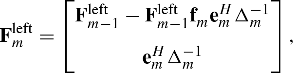
 and
and  ; the initial recursion value is
  . Similarly, the right pseudo-inverse matrix
  has the following recursive formula [39]:
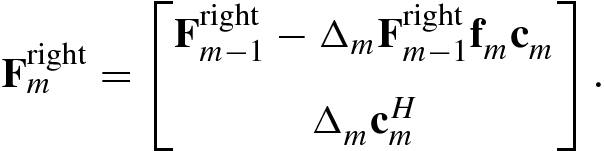
 and
and  . The initial recursion value is
  .
.1.6.3 Moore–Penrose Inverse Matrices
Given an m × n rank-deficient matrix A, regardless of the size of m and n but with  . The inverse of an m × n rank-deficient matrix is said to be its generalized inverse matrix, denoted as A
†, that is an n × m matrix.
. The inverse of an m × n rank-deficient matrix is said to be its generalized inverse matrix, denoted as A
†, that is an n × m matrix.
- 1.If A † is the generalized inverse of A, then Ax = y ⇒x = A †y. Substituting x = A †y into Ax = y, we have AA †y = y, and thus AA †Ax = Ax. Since this equation should hold for any given nonzero vector x, A † must satisfy the condition:
 (1.6.31)
 - 2.Given any y ≠ 0, the solution equation of the original matrix equation, x = A †y, can be written as x = A †Ax, yielding A †y = A †AA †y. Since A †y = A †AA †y should hold for any given nonzero vector y, the second condition
 (1.6.32)
must be satisfied as well.
- 3.If an m × n matrix A is of full column rank or full row rank, we certainly hope that the generalized inverse matrix A † will include the left and right pseudo-inverse matrices as two special cases. Because the left and right pseudo-inverse matrix L = (A HA)−1A H and R = A H(AA H)−1 of the m × n full column rank matrix A satisfy, respectively, AL = A(A HA)−1A H = (AL)H and RA = A H(AA H)−1A = (RA)H, in order to guarantee that A † exists uniquely for any m × n matrix A, the following two conditions must be added:
 (1.6.33)
- (a)
AA †A = A;
- (b)
A †AA † = A †;
- (c)
AA † is an m × m Hermitian matrix, i.e., AA † = (AA †)H;
- (d)
A †A is an n × n Hermitian matrix, i.e., A †A = (A †A)H.
From the projection viewpoint, Moore [23] showed in 1935 that the generalized inverse matrix A † of an m × n matrix A must meet two conditions, but these conditions are not convenient for practical use. After two decades, Penrose [26] in 1955 presented the four conditions (a)–(d) stated above. In 1956, Rado [32] showed that the four conditions of Penrose are equivalent to the two conditions of Moore. Therefore the conditions (a)–(d) are called the Moore–Penrose conditions, and the generalized inverse matrix satisfying the Moore–Penrose conditions is referred to as the Moore–Penrose inverse of A.
It is easy to know that the inverse A −1, the left pseudo-inverse matrix (A HA)−1A H, and the right pseudo-inverse matrix A H(AA H)−1 are special examples of the Moore–Penrose inverse A †.


 , there are the following three methods for computing the Moore–Penrose inverse matrix A
†.
, there are the following three methods for computing the Moore–Penrose inverse matrix A
†. - 1.Equation-solving method [26]
Solve the matrix equations AA HX H = A and A HAY = A H to yield the solutions X H and Y, respectively.
Compute the generalized inverse matrix A † = XAY.
- 2.
Full-rank decomposition method: If A = FG, where F m×r is of full column rank and G r×n is of full row rank, then A = FG is called the full-rank decomposition of the matrix A. By Searle [36], a matrix
 with rank(A) = r has the full-rank decomposition A = FG. Therefore, if A = FG is a full-rank decomposition of the m × n matrix A, then A
† = G
†F
† = G
H(GG
H)−1(F
HF)−1F
H.
with rank(A) = r has the full-rank decomposition A = FG. Therefore, if A = FG is a full-rank decomposition of the m × n matrix A, then A
† = G
†F
† = G
H(GG
H)−1(F
HF)−1F
H. - 3.
Recursive methods: Block the matrix A m×n into A k = [A k−1, a k], where A k−1 consists of the first k − 1 columns of A and a k is the kth column of A. Then, the Moore–Penrose inverse
 of the block matrix A
k can be recursively calculated from
of the block matrix A
k can be recursively calculated from  . When k = n, we get the Moore–Penrose inverse matrix A
†. Such a recursive algorithm was presented by Greville in 1960 [11].
. When k = n, we get the Moore–Penrose inverse matrix A
†. Such a recursive algorithm was presented by Greville in 1960 [11].
- 1.
For an m × n matrix A, its Moore–Penrose inverse A † is uniquely determined.
- 2.
The Moore–Penrose inverse of the complex conjugate transpose matrix A H is given by (A H)† = (A †)H = A †H = A H†.
- 3.
The generalized inverse of a Moore–Penrose inverse matrix is equal to the original matrix, namely (A †)† = A.
- 4.
If c ≠ 0, then (cA)† = c −1A †.
- 5.
If D = Diag(d 11, …, d nn), then
 , where
  (if d
ii ≠ 0) or
(if d
ii ≠ 0) or  (if d
ii = 0).
(if d
ii = 0). - 6.
The Moore–Penrose inverse of an m × n zero matrix O m×n is an n × m zero matrix, i.e.,
 .
. - 7.
If A H = A and A 2 = A, then A † = A.
- 8.If A = BC, B is of full column rank, and C is of full row rank, then

- 9.
(AA H)† = (A †)HA † and (AA H)†(AA H) = AA †.
- 10.
If the matrices A i are mutually orthogonal, i.e.,
 , then
  .
. - 11.
Regarding the ranks of generalized inverse matrices, one has rank(A †) = rank(A) = rank(A H) = rank(A †A) = rank(AA †) = rank(AA †A) = rank(A †AA †).
- 12.
The Moore–Penrose inverse of any matrix A m×n can be determined by A † = (A HA)†A H or A † = A H(AA H)†.
1.7 Direct Sum and Hadamard Product
This section discusses two special operations of matrices: the direct sum of two or more matrices and the Hadamard product of two matrices.
1.7.1 Direct Sum of Matrices
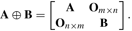
- 1.
If c is a constant, then c (A ⊕B) = cA ⊕ cB.
- 2.
The direct sum does not satisfy exchangeability: A ⊕B ≠ B ⊕A unless A = B.
- 3.If A, B are two m × m matrices and C and D are two n × n matrices, then

- 4.If A, B, C are m × m, n × n, p × p matrices, respectively, then

- 5.
If A m×m and B n×n are, respectively, orthogonal matrices, then A ⊕B is an (m + n) × (m + n) orthogonal matrix.
- 6.The complex conjugate, transpose, complex conjugate transpose, and inverse matrices of the direct sum of two matrices are given by

- 7.The trace, rank, and determinant of the direct sum of N matrices are as follows:

1.7.2 Hadamard Product
![$$\displaystyle \begin{aligned}{}[\mathbf{A}\odot \mathbf{B}]_{ij}=a_{ij} b_{ij}. \end{aligned} $$](../images/492994_1_En_1_Chapter/492994_1_En_1_Chapter_TeX_Equ151.png)
 .
.![$$\displaystyle \begin{aligned}{}[\mathbf{A}\oslash\mathbf{B}]_{ij}=a_{ij}/b_{ij}. \end{aligned} $$](../images/492994_1_En_1_Chapter/492994_1_En_1_Chapter_TeX_Equ152.png)
The following theorem describes the positive definiteness of the Hadamard product and is usually known as the Hadamard product theorem [15].
If two m × m matrices A and B are positive definite (positive semi-definite), then their Hadamard product A ⊙B is positive definite (positive semi-definite) as well.

holds for all m × m positive semi-definite matrices B = [b ij].
The following theorems describe the relationship between the Hadamard product and the matrix trace.
 , where
  ; then

 , while m = M1 is an n × 1 vector. Then one has


- 1.If A, B are m × n matrices, then

- 2.
The Hadamard product of a matrix A m×n and a zero matrix O m×n is given by A ⊙O m×n = O m×n ⊙A = O m×n.
- 3.
If c is a constant, then c (A ⊙B) = (cA) ⊙B = A ⊙ (c B).
- 4.
The Hadamard product of two positive definite (positive semi-definite) matrices A, B is positive definite (positive semi-definite) as well.
- 5.The Hadamard product of the matrix A m×m = [a ij] and the identity matrix I m is an m × m diagonal matrix, i.e.,

- 6.If A, B, D are three m × m matrices and D is a diagonal matrix, then

- 7.If A, C are two m × m matrices and B, D are two n × n Matrices, then

- 8.If A, B, C, D are all m × n matrices, then

- 9.
If A, B, C are m × n matrices, then
 .
.
The Hadamard (i.e., elementwise) products of two matrices are widely used in machine learning, neural networks, and evolutionary computations.
1.8 Kronecker Products
The Hadamard product described in the previous section is a special product of two matrices. In this section, we discuss another special product of two matrices: the Kronecker products. The Kronecker product is also known as the direct product or tensor product [20].
1.8.1 Definitions of Kronecker Products
Kronecker products are divided into right and left Kronecker products.
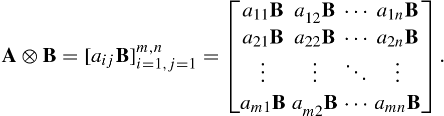
![$$\mathbf {A}=[{\mathbf {a}}_1^{\,} , \ldots ,{\mathbf {a}}_n ]$$](../images/492994_1_En_1_Chapter/492994_1_En_1_Chapter_TeX_IEq183.png) and another p × q matrix B, their right Kronecker product A ⊗B is an mp × nq matrix defined by
and another p × q matrix B, their right Kronecker product A ⊗B is an mp × nq matrix defined by
![$$\mathbf {B}=[{\mathbf {b}}_1^{\,} ,\ldots ,{\mathbf {b}}_q ]$$](../images/492994_1_En_1_Chapter/492994_1_En_1_Chapter_TeX_IEq184.png) , their left Kronecker product A ⊗B is an mp × nq matrix defined by
, their left Kronecker product A ⊗B is an mp × nq matrix defined by
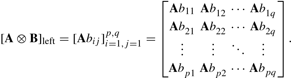
Clearly, the left or right Kronecker product is a mapping  . It is easily seen that the left and right Kronecker products have the following relationship: [A ⊗B]left = B ⊗A. Since the right Kronecker product form is the one generally adopted, this book uses the right Kronecker product hereafter unless otherwise stated.
 and
and  :
: 
1.8.2 Performance of Kronecker Products
- 1.
The Kronecker product of any matrix and a zero matrix is equal to the zero matrix, i.e., A ⊗O = O ⊗A = O.
- 2.
If α and β are constants, then αA ⊗ βB = αβ(A ⊗B).
- 3.
The Kronecker product of an m × m identity matrix and an n × n identity matrix is equal to an mn × mn identity matrix, i.e., I m ⊗I n = I mn.
- 4.For matrices A m×n, B n×k, C l×p, D p×q, we have
 (1.8.4)
 - 5.For matrices A m×n, B p×q, C p×q, we have
 (1.8.5)
 (1.8.6)
 - 6.The inverse and generalized inverse matrix of Kronecker products satisfy
 (1.8.7)
 - 7.The transpose and the complex conjugate transpose of Kronecker products are given by
 (1.8.8)
 - 8.The rank of the Kronecker product is
 (1.8.9)
 - 9.The determinant of the Kronecker product
 (1.8.10)
 - 10.The trace of the Kronecker product is given by
 (1.8.11)
 - 11.For matrices A m×n, B m×n, C p×q, D p×q, we have
 (1.8.12)
 - 12.For matrices A m×n, B p×q, C k×l, it is true that
 (1.8.13)
 - 13.
For matrices A m×n, B p×q, we have
 .
. - 14.


1.9 Vectorization and Matricization
Consider the operators that transform a matrix into a vector or vice versa.
1.9.1 Vectorization and Commutation Matrix
The function or operator that transforms a matrix into a vector is known as the vectorization of the matrix.
 , denoted vec(A), is a linear transformation that arranges the entries of A = [a
ij] as an mn × 1 vector via column stacking:
, denoted vec(A), is a linear transformation that arranges the entries of A = [a
ij] as an mn × 1 vector via column stacking:
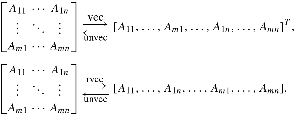
![$$\displaystyle \begin{aligned} \mathrm{vec}(\mathbf{A})=[a_{11},\ldots ,a_{m1},\ldots ,a_{1n},\ldots ,a_{mn}]^T. \end{aligned} $$](../images/492994_1_En_1_Chapter/492994_1_En_1_Chapter_TeX_Equ178.png)
![$$\displaystyle \begin{aligned} \mathrm{rvec}(\mathbf{A})=[a_{11},\ldots ,a_{1n},\ldots ,a_{m1},\ldots , a_{mn}]. \end{aligned} $$](../images/492994_1_En_1_Chapter/492994_1_En_1_Chapter_TeX_Equ179.png)
For instance, given a matrix  , then vec(A) = [a
11, a
21, a
12, a
22]T and rvec(A) = [a
11, a
12, a
21, a
22].
, then vec(A) = [a
11, a
21, a
12, a
22]T and rvec(A) = [a
11, a
12, a
21, a
22].
The column vectorization is usually called the vectorization simply.


From (1.9.4) and (1.9.5) it can be seen that K
nmK
mnvec(A) = K
nmvec(A
T) = vec(A). Since this formula holds for any m × n matrix A, we have K
nmK
mn = I
mn or  .
.
- 1.
K mnvec(A) = vec(A T) and K nmvec(A T) = vec(A), where A is an m × n matrix.
- 2.
 , or
, or  .
. - 3.
 .
. - 4.K mn can be represented as a Kronecker product of the basic vectors:

- 5.
K 1n = K n1 = I n.
- 6.
K nmK mnvec(A) = K nmvec(A T) = vec(A).
- 7.
Eigenvalues of the commutation matrix K nn are 1 and − 1 and their multiplicities are, respectively,
 and
and  .
. - 8.
The rank of the commutation matrix is given by rank(K mn) = 1 + d(m − 1, n − 1), where d(m, n) is the greatest common divisor of m and n, d(n, 0) = d(0, n) = n.
- 9.
K mn(A ⊗B)K pq = B ⊗A, and thus can be equivalently written as K mn(A ⊗B) = (B ⊗A)K qp, where A is an n × p matrix and B is an m × q matrix. In particular, K mn(A n×n ⊗B m×m) = (B ⊗A)K mn.
- 10.
 .
.

![$$\displaystyle \begin{aligned} {\mathbf{K}}_i =[\mathbf{0},{\mathbf{K}}_{i-1}(1:mn-1)],\quad \ i=2,\ldots ,m, \end{aligned} $$](../images/492994_1_En_1_Chapter/492994_1_En_1_Chapter_TeX_Equ185.png)
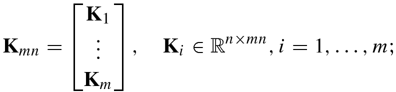
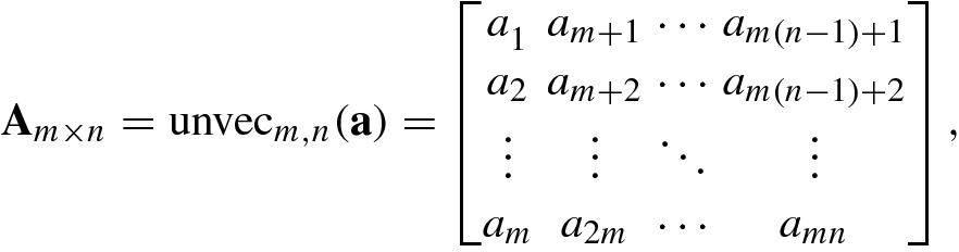
1.9.2 Matricization of Vectors
![$$\mathbf {a}=[a_1^{\,} ,\ldots ,a_{mn}]^T$$](../images/492994_1_En_1_Chapter/492994_1_En_1_Chapter_TeX_IEq200.png) into an m × n matrix A is known as the matricization of column vector or unfolding of column vector, denoted unvecm,n(a), and is defined as
into an m × n matrix A is known as the matricization of column vector or unfolding of column vector, denoted unvecm,n(a), and is defined as

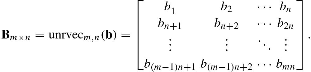
![$$\mathbf {b}=[b_1^{\,} ,\ldots ,b_{mn}]$$](../images/492994_1_En_1_Chapter/492994_1_En_1_Chapter_TeX_IEq201.png) into an m × n matrix B is called the matricization of row vector or unfolding of row vector, denoted unrvecm,n(b), and is defined as
into an m × n matrix B is called the matricization of row vector or unfolding of row vector, denoted unrvecm,n(b), and is defined as


- 1.
The vectorization of a transposed matrix is given by vec(A T) = K mnvec(A) for
 .
. - 2.
The vectorization of a matrix sum is given by vec(A + B) = vec(A) + vec(B).
- 3.The vectorization of a Kronecker product is given by Magnus and Neudecker [22, p. 184]:
 (1.9.15)
 - 4.The trace of a matrix product is given by
 (1.9.16)
 (1.9.17)
 (1.9.18)while the trace of the product of four matrices is determined by Magnus and Neudecker [22, p. 31]:
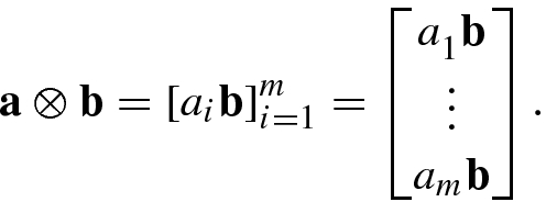
- 5.The Kronecker product of two vectors a and b can be represented as the vectorization of their outer product ba T as follows:
 (1.9.19)
 - 6.The vectorization of the Hadamard product is given by
 (1.9.20)
where Diag(vec(A)) is a diagonal matrix whose entries are the vectorization function vec(A).
- 7.The relation of the vectorization of the matrix product A m×pB p×qC q×n to the Kronecker product is given by Schott [35, p. 263]:
 (1.9.21)
 (1.9.22)
 (1.9.23)
 ,
,  , and
, and  . By using the vectorization function property vec(AXB) = (B
T ⊗A) vec(X), the vectorization vec(AXB) = vec(C) of the original matrix equation can be, in Kronecker product form, rewritten as [33]:
. By using the vectorization function property vec(AXB) = (B
T ⊗A) vec(X), the vectorization vec(AXB) = vec(C) of the original matrix equation can be, in Kronecker product form, rewritten as [33]: 
This chapter focuses on basic operations and performance of matrices, which constitute the foundation of matrix algebra.
Trace, rank, positive definiteness, Moore–Penrose inverse matrices, Kronecker product, Hadamard product (elementwise product), and vectorization of matrices are frequently used in artificial intelligence.