The matrix differential is a generalization of the multivariate function differential. The matrix differential (including the matrix partial derivative and gradient) is an important operation tool in matrix algebra and optimization in machine learning, neural networks, support vector machine and evolutional computation. This chapter is concerned with the theory and methods of matrix differential.
2.1 Jacobian Matrix and Gradient Matrix
Symbols of real functions
Function type | Variable | Variable |
|---|---|---|
Scalar function |
|
|
Vector function |
|
|
Matrix function |
|
|


2.1.1 Jacobian Matrix
- 1.Row partial derivative operator with respect to an m × 1 vector is defined as
![$$\displaystyle \begin{aligned} {\boldsymbol \nabla}_{{\mathbf{x}}^T}^{\,} \stackrel{\mathrm{def}}{=} \frac{\partial}{\partial\,{\mathbf{x}}^T}=\left [\frac{\partial}{\partial x_1^{\,}},\ldots ,\frac{\partial}{\partial x_m^{\,}}\right ],{} \end{aligned} $$](../images/492994_1_En_2_Chapter/492994_1_En_2_Chapter_TeX_Equ1.png) (2.1.1)and row partial derivative vector of real scalar function f(x) with respect to its m × 1 vector variable x is given by
(2.1.1)and row partial derivative vector of real scalar function f(x) with respect to its m × 1 vector variable x is given by![$$\displaystyle \begin{aligned} {\boldsymbol \nabla}_{{\mathbf{x}}^T}^{\,} f(\mathbf{x})=\frac{\partial f(\mathbf{x})}{\partial\,{\mathbf{x}}^T}=\left [\frac{\partial f(\mathbf{x})} {\partial x_1^{\,}},\ldots , \frac{\partial f(\mathbf{x})}{\partial x_m^{\,}}\right ].{} \end{aligned} $$](../images/492994_1_En_2_Chapter/492994_1_En_2_Chapter_TeX_Equ2.png) (2.1.2)
(2.1.2) - 2.Row partial derivative operator with respect to an m × n matrix X is defined as
![$$\displaystyle \begin{aligned} {\boldsymbol \nabla}_{(\mathrm{vec}\,\mathbf{X})^T}\stackrel{\mathrm{def}}{=}\frac{\partial}{\partial (\mathrm{vec}\,\mathbf{X})^T}=\left [\frac{\partial} {\partial x_{11}^{\,}},\ldots ,\frac{\partial}{\partial x_{m1}^{\,}},\ldots ,\frac{\partial}{\partial x_{1n}^{\,}},\ldots ,\frac{\partial}{\partial x_{mn}^{\,}} \right ], \end{aligned} $$](../images/492994_1_En_2_Chapter/492994_1_En_2_Chapter_TeX_Equ3.png) (2.1.3)and row partial derivative vector of real scalar function f(X) with respect to its matrix variable
(2.1.3)and row partial derivative vector of real scalar function f(X) with respect to its matrix variable is given by
 ![$$\displaystyle \begin{aligned} {\boldsymbol \nabla}_{(\mathrm{vec}\,\mathbf{X})^T}^{\,} f(\mathbf{X})\!=\!\frac{\partial f(\mathbf{X})}{\partial (\mathrm{vec}\,\mathbf{X})^T}\!=\!\left [\frac{\partial f(\mathbf{X} )} {\partial x_{11}^{\,}},\ldots ,\frac{\partial f( \mathbf{X})}{\partial x_{m1}^{\,}},\ldots ,\frac {\partial f(\mathbf{X})}{\partial x_{1n}^{\,}},\ldots , \frac{\partial f(\mathbf{X})}{\partial x_{mn}^{\,}} \right ]{}. \end{aligned} $$](../images/492994_1_En_2_Chapter/492994_1_En_2_Chapter_TeX_Equ4.png) (2.1.4)
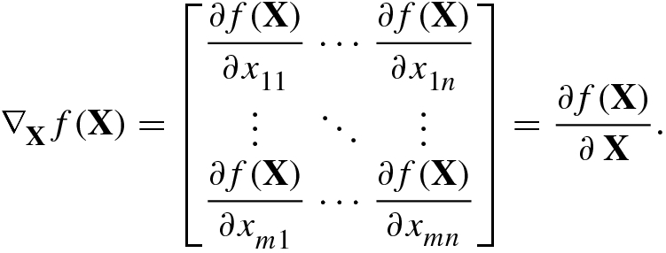
(2.1.4) - 3.Jacobian operator with respect to an m × n matrix X is defined as
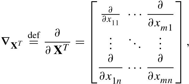 (2.1.5)and Jacobian matrix of the real scalar function f(X) with respect to its matrix variable
 is given by
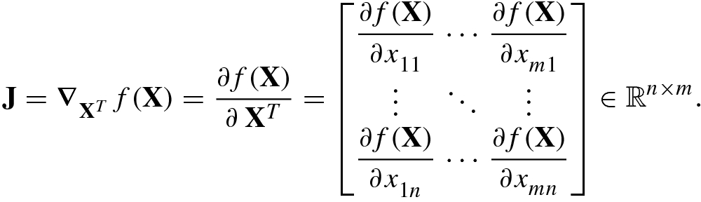 (2.1.6)

As a matter of fact, the Jacobian matrix is more useful than the row partial derivative vector.
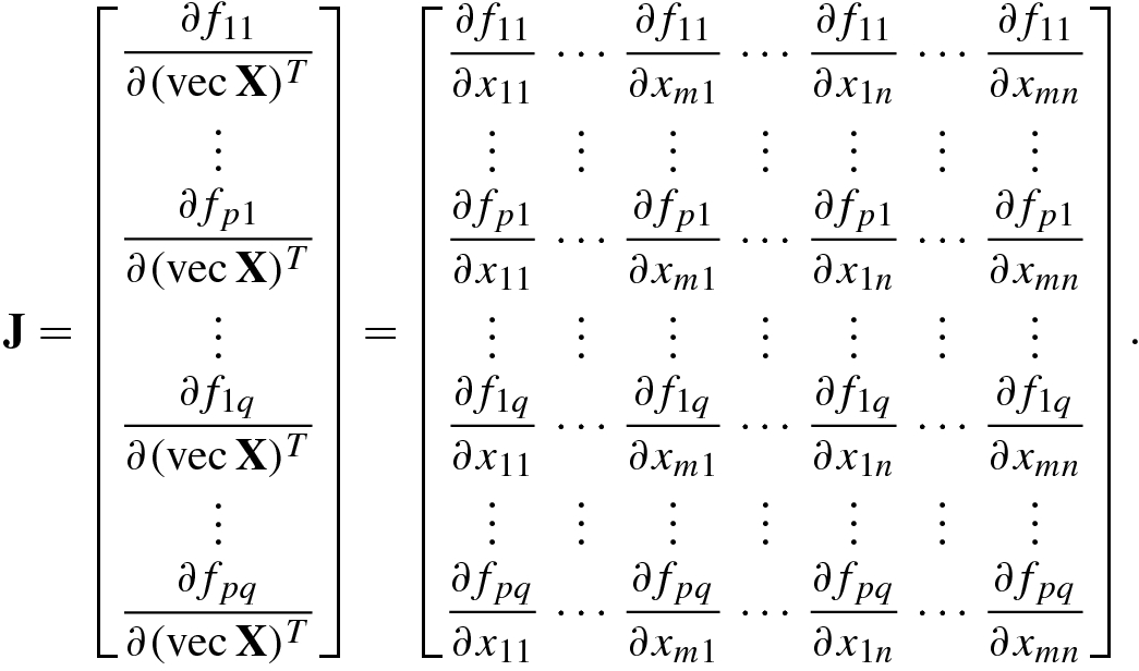
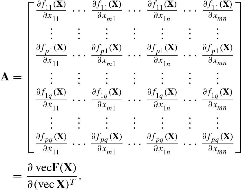
The following theorem provides a specific expression for the Jacobian matrix of a p × q real-valued matrix function F(X) with m × n matrix variable X.
![$$\displaystyle \begin{aligned} \mathrm{vec}\, \mathbf{F}(\mathbf{X})\stackrel{\mathrm{def}}{=}[f_{11}(\mathbf{X}),\ldots ,f_{p1}(\mathbf{X}), \ldots , f_{1q}(\mathbf{X}),\ldots ,f_{pq}(\mathbf{X})]^T\ \in\mathbb{R}^{pq}. \end{aligned} $$](../images/492994_1_En_2_Chapter/492994_1_En_2_Chapter_TeX_Equ8.png)

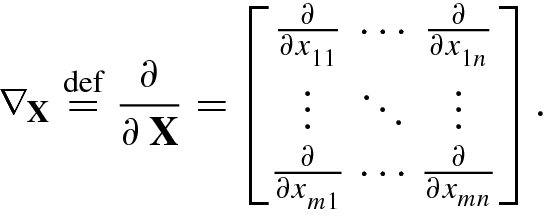
2.1.2 Gradient Matrix
The partial derivative operator in column form is referred to as the gradient vector operator.
![$$\displaystyle \begin{aligned} \nabla_{\mathbf{x}}^{\,} \stackrel{\mathrm{def}}{=} \frac{\partial}{\partial\,\mathbf{x}}=\left [\frac{\partial}{\partial x_1^{\,}}, \ldots , \frac{\partial}{\partial x_m^{\,}}\right ]^T \end{aligned} $$](../images/492994_1_En_2_Chapter/492994_1_En_2_Chapter_TeX_Equ11.png)
![$$\displaystyle \begin{aligned} \nabla_{\mathrm{vec}\,\mathbf{X}}^{\,} \stackrel{\mathrm{def}}{=}\frac{\partial}{\partial\,\mathrm{vec}\,\mathbf{X}}=\left [\frac{\partial}{\partial x_{11}^{\,}},\ldots ,\frac{\partial}{\partial x_{1n}^{\,}},\ldots ,\frac {\partial}{\partial x_{m1}^{\,}},\ldots ,\frac{\partial} {\partial x_{mn}^{\,}} \right ]^T. \end{aligned} $$](../images/492994_1_En_2_Chapter/492994_1_En_2_Chapter_TeX_Equ12.png)
 , is defined as
![$$\displaystyle \begin{aligned} \nabla_{\mathbf{x}}^{\,} f(\mathbf{x})&\stackrel{\mathrm{def}}{=}\left [\frac {\partial f( \mathbf{x})}{\partial x_1^{\,}}, \ldots ,\frac{\partial f( \mathbf{x})}{\partial x_m^{\,}}\right ]^T= \frac {\partial f( \mathbf{x})}{\partial\mathbf{x}}, \end{aligned} $$](../images/492994_1_En_2_Chapter/492994_1_En_2_Chapter_TeX_Equ14.png)
![$$\displaystyle \begin{aligned} \nabla_{\mathrm{vec}\,\mathbf{X}}^{\,} f(\mathbf{X})&\stackrel{\mathrm{def}}{=}\left [\frac{\partial f(\mathbf{X})}{\partial x_{11}^{\,}}, \ldots ,\frac{\partial f(\mathbf{X})}{\partial x_{m1}^{\,}},\ldots ,\frac{\partial f(\mathbf{X})}{\partial x_{1n}^{\,}},\ldots , \frac{\partial f(\mathbf{X})}{\partial x_{mn}^{\,}} \right ]^T. \end{aligned} $$](../images/492994_1_En_2_Chapter/492994_1_En_2_Chapter_TeX_Equ15.png)
 with matrix variable
  , its gradient matrix is defined as


An obvious fact is that, given a real scalar function f(x), its gradient vector is directly equal to the transpose of the partial derivative vector. In this sense, the partial derivative in row vector form is a covariant form of the gradient vector, so the row partial derivative vector is also known as the cogradient vector. Similarly, the Jacobian matrix is sometimes called the cogradient matrix. The cogradient is a covariant operator [3] that itself is not the gradient, but is related to the gradient.
For this reason, the partial derivative operator ∂∕∂x T and the Jacobian operator ∂∕∂ X T are known as the (row) partial derivative operator, the covariant form of the gradient operator or the cogradient operator.
 is known as the gradient flow direction of the function f(x) at the point x, and is expressed as

In the gradient flow direction, the function f(x) decreases at the maximum descent rate. On the contrary, in the opposite direction (i.e., the positive gradient direction), the function increases at the maximum ascent rate.
Each component of the gradient vector gives the rate of change of the scalar function f(x) in the component direction.
2.1.3 Calculation of Partial Derivative and Gradient
- 1.
If f(X) = c, where c is a real constant and X is an m × n real matrix, then the gradient
 .
. - 2.Linear rule: If f(X) and g(X) are two real-valued functions of the matrix variable X, and
 and
and  are two real constants, then
![$$\displaystyle \begin{aligned} \begin{aligned} \frac{\partial [c_1^{\,} f(\mathbf{X})+c_2^{\,} g( \mathbf{X})]}{\partial\mathbf{X}}= c_1^{\,} \frac{\partial f(\mathbf{X})} {\partial\,\mathbf{X}}+c_2^{\,}\frac{\partial g(\mathbf{X})}{\partial\mathbf{X}} \end{aligned} . \end{aligned} $$](../images/492994_1_En_2_Chapter/492994_1_En_2_Chapter_TeX_Equ21.png) (2.1.21)
(2.1.21) - 3.Product rule: If f(X), g(X), and h(X) are real-valued functions of the matrix variable X, then
 (2.1.22)and
 (2.1.23)
 - 4.Quotient rule: If g(X) ≠ 0, then
 (2.1.24)
 - 5.Chain rule: If X is an m × n matrix and y = f(X) and g(y) are, respectively, the real-valued functions of the matrix variable X and of the scalar variable y, then
 (2.1.25)
![$$\mathbf {F}=[f_{kl}]\in \mathbb {R}^{p\times q}$$](../images/492994_1_En_2_Chapter/492994_1_En_2_Chapter_TeX_IEq21.png) and
and ![$$\mathbf {X}=[x_{ij}]\in \mathbb {R}^{m\times n}$$](../images/492994_1_En_2_Chapter/492994_1_En_2_Chapter_TeX_IEq22.png) , then the chain rule is given by Petersen and Petersen [7]
, then the chain rule is given by Petersen and Petersen [7] ![$$\displaystyle \begin{aligned} \left [\frac{\partial g(\mathbf{F})}{\partial\,\mathbf{X}}\right ]_{ij}=\frac{\partial g(\mathbf{F})}{\partial x_{ij}}= \sum_{k=1}^p\sum_{l=1}^q \frac {\partial g(\mathbf{F})}{\partial f_{kl}}\frac{\partial f_{kl}}{\partial x_{ij}}. \end{aligned} $$](../images/492994_1_En_2_Chapter/492994_1_En_2_Chapter_TeX_Equ26.png)
When computing the partial derivative of the functions f(x) and f(X), it is necessary to make the following basic assumption.
Given a real-valued function f, we assume that the vector variable ![$$\mathbf {x}=[x_i^{\,} ]_{i=1}^m\in \mathbb {R}^m$$](../images/492994_1_En_2_Chapter/492994_1_En_2_Chapter_TeX_IEq23.png) and the matrix variable
and the matrix variable ![$$\mathbf {X}=[x_{ij}^{\,} ]_{i=1, j=1}^{m,n}\in \mathbb {R}^{m \times n}$$](../images/492994_1_En_2_Chapter/492994_1_En_2_Chapter_TeX_IEq24.png) do not themselves have any special structure; namely, the entries of x (and X) are independent.
do not themselves have any special structure; namely, the entries of x (and X) are independent.


These expressions on independence are the basic formulas for partial derivative computation.

![$$\displaystyle \begin{aligned} \left[\frac{\partial f(\mathbf{X})}{\partial\,{\mathbf{X}}^T}\right]_{ij}&=\frac{\partial f(\mathbf{X})}{\partial x_{ji}}= \sum_{k=1}^m\sum_{l=1}^m \sum_{p=1}^n \frac{\partial a_k^{\,} x_{kp}x_{lp}b_l^{\,}}{\partial x_{ji}}\\ &=\sum_{k=1}^m \sum_{l=1}^m \sum_{p=1}^n\left [ a_k^{\,} x_{lp}b_l^{\,}\frac{\partial x_{kp}}{\partial x_{ji}}+a_k^{\,} x_{kp} b_l^{\,} \frac{\partial x_{lp}}{\partial x_{ji}}\right ]\\ &=\sum_{i=1}^m\sum_{l=1}^m \sum_{j=1}^n a_j^{\,} x_{li}b_l^{\,} + \sum_{k=1}^m \sum_{i=1}^m \sum_{j=1}^n a_k^{\,} x_{ki} b_j^{\,} \\ &=\sum_{i=1}^m\sum_{j=1}^n \left [{\mathbf{X}}^T\mathbf{b} \right]_i a_j^{\,} +\left [{\mathbf{X}}^T\mathbf{a}\right ]_i b_j^{\,} , \end{aligned} $$](../images/492994_1_En_2_Chapter/492994_1_En_2_Chapter_TeX_Equb.png)

 . We have
 ![$$\displaystyle \begin{aligned} &\frac{\partial f_{kl}^{\,}}{\partial x_{ij}^{\,}}=\frac{\partial [\mathbf{AXB}]_{kl}}{\partial x_{ij}^{\,}}=\frac{\partial \left (\sum_{u=1}^m \sum_{v=1}^n a_{ku}^{\,} x_{uv}^{\,} b_{vl}^{\,}\right )}{\partial x_{ij}}=b_{jl}^{\,} a_{ki}^{\,}\\ \Rightarrow&~\nabla_{\mathbf{X}}^{\,} (\mathbf{AXB})= \mathbf{B}\otimes {\mathbf{A}}^T~~ \Rightarrow~~ \mathbf{J}=(\nabla_{\mathbf{X}}^{\,} (\mathbf{AXB}))^T={\mathbf{B}}^T\otimes \mathbf{A}. \end{aligned} $$](../images/492994_1_En_2_Chapter/492994_1_En_2_Chapter_TeX_Equd.png)
 .
.2.2 Real Matrix Differential
Although direct computation of partial derivatives  or
or  can be used to find the Jacobian matrices or the gradient matrices of many matrix functions, for more complex functions (such as the inverse matrix, the Moore–Penrose inverse matrix and the exponential functions of a matrix), direct computation of their partial derivatives is more complicated and difficult. Hence, naturally we want to have an easily remembered and effective mathematical tool for computing the Jacobian matrices and the gradient matrices of real scalar functions and real matrix functions. Such a mathematical tool is the matrix differential.
2.2.1 Calculation of Real Matrix Differential
The differential of an m × n matrix ![$$\mathbf {X}=[x_{ij}^{\,} ]$$](../images/492994_1_En_2_Chapter/492994_1_En_2_Chapter_TeX_IEq29.png) is known as the matrix differential, denoted dX, which is still m × n matrix and is defined as
is known as the matrix differential, denoted dX, which is still m × n matrix and is defined as ![$$\mathrm {d} \mathbf {X}=[\mathrm {d}x_{ij}^{\,} ]_{i=1,j=1}^{m,n}$$](../images/492994_1_En_2_Chapter/492994_1_En_2_Chapter_TeX_IEq30.png) .
.

![$$\displaystyle \begin{aligned}{}[\mathrm{d}(\mathbf{UV})]_{ij}^{\,} &=\mathrm{d}\left ( [\mathbf{UV}]_{ij}^{\,}\right )=\mathrm{d} \bigg( \sum_k u_{ik}^{\,} v_{kj}^{\,}\bigg) =\sum_k \mathrm{d}(u_{ik}^{\,} v_{kj}^{\,} )\\ &=\sum_k \left ( (\mathrm{d}u_{ik}^{\,} )v_{kj}^{\,} +u_{ik}^{\,} \mathrm{d}v_{kj}^{\,} \right )=\sum_k (\mathrm{d}u_{ik}^{\,} )v_{kj}^{\,} + \sum_k u_{ik}^{\,} \mathrm{d} v_{kj}^{\,}\\ &=[(\mathrm{d}\mathbf{U})\mathbf{V} ]_{ij}^{\,} + [\mathbf{U}(\mathrm{d}\mathbf{V})]_{ij}^{\,} . \end{aligned} $$](../images/492994_1_En_2_Chapter/492994_1_En_2_Chapter_TeX_Equf.png)
- 1.
The differential of a constant matrix is a zero matrix, namely dA = O.
- 2.
The matrix differential of the product αX is given by d(αX) = α dX.
- 3.
The matrix differential of a transposed matrix is equal to the transpose of the original matrix differential, namely d(X T) = (dX)T.
- 4.
The matrix differential of the sum (or difference) of two matrices is given by d(U ±V) = dU ±dV. More generally, we have d(aU ± bV) = a ⋅dU ± b ⋅dV.
- 5.The matrix differentials of the functions UV and UVW, where U = F(X), V = G(X), W = H(X), are, respectively, given by
 (2.2.1)
 (2.2.2)
If A and B are constant matrices, then d(AXB) = A(dX)B.
- 6.The differential of the matrix trace d(tr X) is equal to the trace of the matrix differential dX, namely
 (2.2.3)
In particular, the differential of the trace of the matrix function F(X) is given by d(tr F(X)) = tr(dF(X)).
- 7.The differential of the determinant of X is given by
 (2.2.4)
In particular, the differential of the determinant of the matrix function F(X) is computed by d|F(X)| = |F(X)|tr(F −1(X)dF(X)).
- 8.The matrix differential of the Kronecker product is given by
 (2.2.5)
 - 9.The matrix differential of the Hadamard product is computed by
 (2.2.6)
 - 10.The matrix differential of the inverse matrix is given by
 (2.2.7)
 - 11.The differential of the vectorization function vec X is equal to the vectorization of the matrix differential, i.e.,
 (2.2.8)
 - 12.The differential of the matrix logarithm is given by
 (2.2.9)
In particular,
 .
. - 13.The matrix differentials of X †, X †X, and XX † are given by
 (2.2.10)
 (2.2.11)
 (2.2.12)
2.2.2 Jacobian Matrix Identification
 is said to be differentiable at the point
  , if a change in
  can be expressed as
 are independent of
  , respectively, and
 denotes the second-order and the higher-order terms in
  . In this case, the partial derivative
  must exist, and
 ,
, 
 and is denoted by

The sufficient condition for a multivariate function  to be differentiable at the point
  is that the partial derivatives
  exist and are continuous.
- For a scalar function f(x) with variable
![$$\mathbf {x}=[x_1^{\,} ,\ldots ,x_m^{\,} ]^T\in \mathbb {R}^m$$](../images/492994_1_En_2_Chapter/492994_1_En_2_Chapter_TeX_IEq46.png) , if regarding the elements
, if regarding the elements  as m variables, and using Eq. (2.2.13), then we can directly obtain the differential of the scalar function f(x) as follows: or
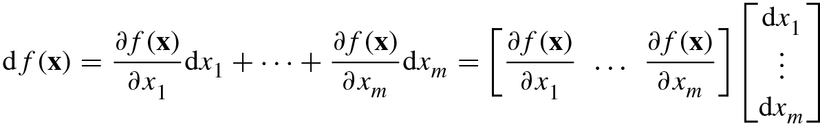 where
where (2.2.14)
![$$\frac {\partial f(\mathbf {x})}{\partial \,{\mathbf {x}}^T}=\Big [\frac {\partial f(\mathbf {x})}{\partial x_1}, \ldots , \frac {\partial f(\mathbf {x})}{\partial x_m}\Big ]$$](../images/492994_1_En_2_Chapter/492994_1_En_2_Chapter_TeX_IEq48.png) and dx = [dx
1, …, dx
m]T. If denoting the row vector
and dx = [dx
1, …, dx
m]T. If denoting the row vector  , then the first-order differential in (2.2.14) can be represented as a trace: because Adx is a scalar, and for any scalar α we have α = tr(α). This shows that there is an equivalence relationship between the Jacobian matrix of the scalar function f(x) and its matrix differential as follows:
 In other words, if the differential of the function f(x) is denoted as df(x) = tr(A dx), then the matrix A is just the Jacobian matrix of the function f(x).
 (2.2.15)
 - For a scalar function f(X) with variable
![$$\mathbf {X}=[{\mathbf {x}}_1^{\,} ,\ldots ,{\mathbf {x}}_n^{\,} ]\in \mathbb {R}^{m\times n}$$](../images/492994_1_En_2_Chapter/492994_1_En_2_Chapter_TeX_IEq50.png) , if denoting
, if denoting ![$${\mathbf {x}}_j^{\,} =[ x_{1j}^{\,} ,\ldots ,x_{mj}^{\,} ]^T, j=1,\ldots ,n$$](../images/492994_1_En_2_Chapter/492994_1_En_2_Chapter_TeX_IEq51.png) , then Eq. (2.2.13) becomes By the relationship between the row partial derivative vector and the Jacobian matrix in Eq. (2.1.7),
, then Eq. (2.2.13) becomes By the relationship between the row partial derivative vector and the Jacobian matrix in Eq. (2.1.7),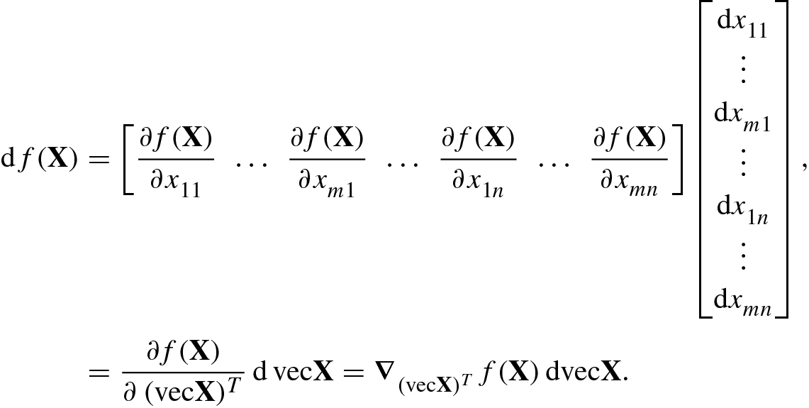 (2.2.16)
 , Eq. (2.2.16) can be written as where
 (2.2.17)is the Jacobian matrix of the scalar function f(X). Using the relationship between the vectorization operator vec and the trace function tr(B TC) = (vec B)Tvec C, and letting B = A T and C = dX, then Eq. (2.2.17) can be expressed in the trace form as
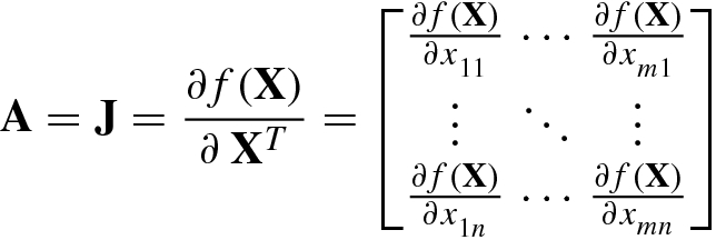 (2.2.18)This can be regarded as the canonical form of the differential of a scalar function f(X).
 (2.2.19)
The above discussion shows that once the matrix differential of a scalar function df(X) is expressed in its canonical form, we can identify the Jacobian matrix and/or the gradient matrix of the scalar function f(X), as stated below.


 of the scalar function f(X):
 - 1.
Find the differential df(X) of the real function f(X), and denote it in the canonical form as df(X) = tr(A dX).
- 2.
The Jacobian matrix is directly given by A.
Any scalar function f(X) can always be written in the form of a trace function, because f(X) = tr(f(X)).
No matter where dX appears initially in the trace function, we can place it in the rightmost position via the trace property tr(C(dX)B) = tr(BC dX), giving the canonical form df(X) = tr(A dX).
It has been shown [6] that the Jacobian matrix A is uniquely determined: if there are A 1 and A 2 such that df(X) = A idX, i = 1, 2, then A 1 = A 2.

Example 2.3


Similarly, we can compute the differential matrices and Jacobian matrices of other typical trace functions.
Differential matrices and Jacobian matrices of trace functions
f(X) | Differential df(X) | Jacobian matrix J = ∂f(X)∕∂X |
|---|---|---|
tr(X) | tr(IdX) | I |
tr(X −1) | −tr(X −2dX) | −X −2 |
tr(AX) | tr(AdX) | A |
tr(X 2) | 2tr(XdX) | 2X |
tr(X TX) | 2tr(X TdX) | X T |
tr(X TAX) |
| X T(A + A T) |
tr(XAX T) |
| (A + A T)X T |
tr(XAX) |
| AX + XA |
tr(AX −1) |
| −X −1AX −1 |
tr(AX −1B) |
| −X −1BAX −1 |
|
| − (X + A)−2 |
tr(XAXB) |
| AXB + BXA |
tr(XAX TB) |
| AX TB + A TX TB T |
tr(AXX TB) |
| X T(BA + A TB T) |
tr(AX TXB) |
| (BA + A TB T)X T |


Consider the Jacobian matrix identification of typical determinant functions.
Example 2.4


 . If rank(X) = n, i.e., X
TX is invertible, then
. If rank(X) = n, i.e., X
TX is invertible, then 
Similarly, we can compute the differential matrices and Jacobian matrices of other typical determinant functions.
Differentials and Jacobian matrices of determinant functions
f(X) | Differential df(X) | Jacobian matrix J = ∂f(X)∕∂X |
|---|---|---|
|X| | |X| tr(X −1dX) | |X|X −1 |
| tr(X −1dX) | X −1 |
|X −1| | −|X −1| tr(X −1dX) | −|X −1|X −1 |
|X 2| |
| 2|X|2X −1 |
|X k| | k|X|k tr(X −1dX) | k|X|kX −1 |
|XX T| |
| 2|XX T|X T(XX T)−1 |
|X TX| |
| 2|X TX|(X TX)−1X T |
|
| 2(X TX)−1X T |
|AXB| |
| |AXB|B(AXB)−1A |
|XAX T| |
|
|
|X TAX| |
|
|


2.2.3 Jacobian Matrix of Real Matrix Functions
 be the entry of the kth row and lth column of the real matrix function F(X); then
 ![$$\mathrm {d}f_{kl}(\mathbf {X})=[\mathrm {d} \mathbf {F}(\mathbf {X})]_{kl}^{\,}$$](../images/492994_1_En_2_Chapter/492994_1_En_2_Chapter_TeX_IEq78.png) represents the differential of the scalar function
represents the differential of the scalar function  with respect to the variable matrix X. From Eq. (2.2.16) we have
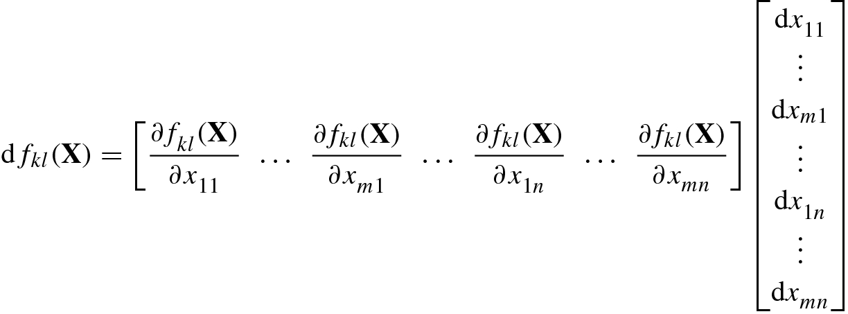

![$$\displaystyle \begin{aligned} \mathrm{d} \mathrm{vec} \mathbf{F}(\mathbf{X})&= [\mathrm{d}f_{11}(\mathbf{X}),\ldots ,\mathrm{d}f_{p1}(\mathbf{X}),\ldots ,\mathrm{d}f_{1q} (\mathbf{X}),\ldots ,\mathrm{d}f_{pq}(\mathbf{X})]^T, \end{aligned} $$](../images/492994_1_En_2_Chapter/492994_1_En_2_Chapter_TeX_Equ55.png)
![$$\displaystyle \begin{aligned} \mathrm{d}\,\mathrm{vec} \mathbf{X}&=[\mathrm{d}x_{11}^{\,} ,\ldots ,\mathrm{d}x_{m1}^{\,} ,\ldots ,\mathrm{d}x_{1n}^{\,} ,\ldots ,\mathrm{d}x_{mn}^{\,} ]^T, \end{aligned} $$](../images/492994_1_En_2_Chapter/492994_1_En_2_Chapter_TeX_Equ56.png)
 of the matrix function F(X).
Let  be a matrix function including X and X
T as variables, where
be a matrix function including X and X
T as variables, where  .
.
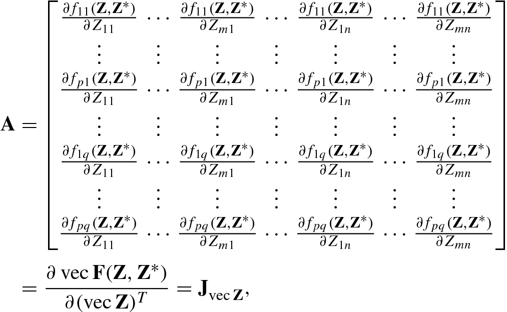
 , then its pq × mn Jacobian matrix can be identified as follows:

Matrix differentials and Jacobian matrices of real functions
Functions | Matrix differential | Jacobian matrix |
|---|---|---|
| df(x) = Adx |
|
| df(x) = Adx |
|
| df(X) = tr(AdX) |
|
| df(x) = Adx |
|
| df(X) = Ad(vecX) |
|
| d vecF(x) = Adx |
|
| dF(X) = A(dX)B + C(dX T)D |
|


Differentials and Jacobian matrices of matrix functions
F(X) | dF(X) | Jacobian matrix |
|---|---|---|
X TX | X TdX + (dX T)X | (I n ⊗X T) + (X T ⊗I n)K mn |
XX T | X(dX T) + (dX)X T | (I m ⊗X)K mn + (X ⊗I m) |
AX TB | A(dX T)B | (B T ⊗A)K mn |
X TBX | X TB dX + (dX T)BX | I ⊗ (X TB) + ((BX)T ⊗I)K mn |
AX TBXC | A(dX T)BXC + AX TB(dX)C | ((BXC)T ⊗A)K mn + C T ⊗ (AX TB) |
AXBX TC | A(dX)BX TC + AXB(dX T)C | (BX TC)T ⊗A + (C T ⊗ (AXB))K mn |
X −1 | −X −1(dX)X −1 | − (X −T ⊗X −1) |
X k |
|
|
| X −1dX | I ⊗X −1 |
|
|
|


 and
and  . Consider the matrix differential dF(X, Y) = (dX) ⊗Y + X ⊗ (dY). By the vectorization formula vec(X ⊗Y) = (I
m ⊗K
qp ⊗I
n)(vec X ⊗vec Y), we have
. Consider the matrix differential dF(X, Y) = (dX) ⊗Y + X ⊗ (dY). By the vectorization formula vec(X ⊗Y) = (I
m ⊗K
qp ⊗I
n)(vec X ⊗vec Y), we have 


The analysis and examples in this section show that the first-order real matrix differential is indeed an effective mathematical tool for identifying the Jacobian matrix and the gradient matrix of a real function. And this tool is simple and easy to master.
2.3 Complex Gradient Matrices
Complex gradient: the gradient of the objective function with respect to the complex vector or matrix variable itself;
Conjugate gradient: the gradient of the objective function with respect to the complex conjugate vector or matrix variable.
2.3.1 Holomorphic Function and Complex Partial Derivative
Before discussing the complex gradient and conjugate gradient, it is necessary to recall the relevant facts about complex functions.
Let  be the definition domain of the function
  . The function f(z) with complex variable z is said to be a complex analytic function in the domain D if f(z) is complex differentiable, namely
  exists for all z ∈ D.
In the standard framework of complex functions, a complex function f(z) (where z = x + jy) is written in the real polar coordinates  as f(r) = f(x, y).
The terminology “complex analytic function” is commonly replaced by the completely synonymous terminology “holomorphic function.” It is noted that a (real) analytic complex function is (real) in the real-variable x-domain and y-domain, but is not necessarily holomorphic in the complex variable domain z = x + jy, i.e., it may be complex nonanalytic.

- 1.
The complex function f(z) is a holomorphic (i.e., complex analytic) function.
- 2.
The derivative f ′(z) of the complex function exists and is continuous.
- 3.The complex function f(z) satisfies the Cauchy–Riemann condition
 (2.3.1)
 - 4.
All derivatives of the complex function f(z) exist, and f(z) has a convergent power series.


A complex function f(z) = u(x, y) + jv(x, y) is not a holomorphic function if any of two real functions u(x, y) and v(x, y) does not meet the Cauchy–Riemann condition or the Laplace equations.
 , the sine function
  , and the cosine function
  are holomorphic functions, i.e., analytic functions in the complex plane, many commonly used functions are not holomorphic. A natural question to ask is whether there is a general representation form f(z, ⋅) instead of f(z) such that f(z, ⋅) is always holomorphic. The key to solving this problem is to adopt f(z, z
∗) instead of f(z), as shown in Table 2.6.
are holomorphic functions, i.e., analytic functions in the complex plane, many commonly used functions are not holomorphic. A natural question to ask is whether there is a general representation form f(z, ⋅) instead of f(z) such that f(z, ⋅) is always holomorphic. The key to solving this problem is to adopt f(z, z
∗) instead of f(z), as shown in Table 2.6. Forms of complex-valued functions
Function | Variables | Variables | Variables |
|---|---|---|---|
|
|
|
|
|
|
|
|
|
|
|
|


Equation (2.3.6) reveals a basic result in the theory of complex variables: the complex variable z and the complex conjugate variable z ∗ are independent variables.
 , the complex variable z and the complex conjugate variable z
∗ can be regarded as two independent variables:
, the complex variable z and the complex conjugate variable z
∗ can be regarded as two independent variables:

Nonholomorphic and holomorphic functions
Functions | Nonholomorphic | Holomorphic |
|---|---|---|
Coordinates |
|
|
Representation | f(r) = f(x, y) | f(c) = f(z, z ∗) |


The function f(z) = |z|2 itself is not a holomorphic function with respect to z, but f(z, z ∗) = |z|2 = zz ∗ is holomorphic, because its first-order partial derivatives ∂|z|2∕∂z = z ∗ and ∂|z|2∕∂z ∗ = z exist and are continuous.
- 1.The conjugate partial derivative of the complex conjugate function
 :
:  (2.3.8)
 - 2.The partial derivative of the conjugate of the complex function
 :
:  (2.3.9)
 - 3.Complex differential rule
 (2.3.10)
 - 4.Complex chain rule
 (2.3.11)
 (2.3.12)
2.3.2 Complex Matrix Differential
Consider the complex matrix function F(Z) and the holomorphic complex matrix function F(Z, Z ∗).
The matrix function F(Z) is a holomorphic function of the complex matrix variable Z.
The complex matrix differential
 .
.For all Z,
 (zero matrix) holds.
For all Z,
 holds.

![$$\mathrm {d}\,\mathbf {Z}=[\mathrm {d}Z_{ij}]_{i=1,j=1}^{m,n}$$](../images/492994_1_En_2_Chapter/492994_1_En_2_Chapter_TeX_IEq136.png) has the following properties [1]:
has the following properties [1]: - 1.
Transpose: dZ T = d(Z T) = (dZ)T.
- 2.
Hermitian transpose: dZ H = d(Z H) = (dZ)H.
- 3.
Conjugate: dZ ∗ = d(Z ∗) = (dZ)∗.
- 4.
Linearity (additive rule): d(Y + Z) = dY + dZ.
- 5.Chain rule: If F is a function of Y, while Y is a function of Z, then

where
 and
and  are the normal complex partial derivative and the generalized complex partial derivative, respectively.
 - 6.Multiplication rule:

- 7.
Kronecker product: d(Y ⊗Z) = dY ⊗Z + Y ⊗dZ.
- 8.
Hadamard product: d(Y ⊙Z) = dY ⊙Z + Y ⊙dZ.
Let us consider the relationship between the complex matrix differential and the complex partial derivative.

 :
: 
![$$\mathrm {d}\mathbf {z}=[\mathrm {d}z_1^{\,} ,\ldots ,\mathrm {d}z_m^{\,}]^T$$](../images/492994_1_En_2_Chapter/492994_1_En_2_Chapter_TeX_IEq140.png) ,
, ![$$\mathrm {d}{\mathbf {z}}^*=[\mathrm {d}z_1^*,\ldots ,\mathrm {d}z_m^* ]^T$$](../images/492994_1_En_2_Chapter/492994_1_En_2_Chapter_TeX_IEq141.png) . This complex differential rule is the basis of the complex matrix differential.
. This complex differential rule is the basis of the complex matrix differential.

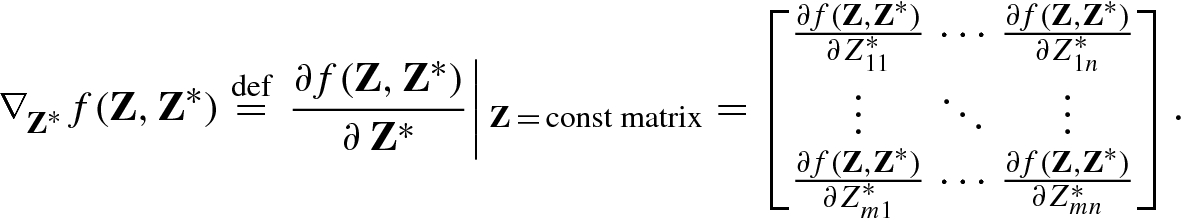
![$$\displaystyle \begin{aligned} \mathrm{D}_{\mathbf{z}}^{\,} f(\mathbf{z},{\mathbf{z}}^*)&=\left .\frac{\partial f(\mathbf{z},{\mathbf{z}}^*)}{\partial\,{\mathbf{z}}^T}\right |{}_{{\mathbf{z}}^* =\mathrm{const}}=\left [\frac {\partial f(\mathbf{z},{\mathbf{z}}^*)}{\partial z_1^{\,}}, \ldots ,\frac{\partial f(\mathbf{z},{\mathbf{z}}^*)} {\partial z_m^{\,}}\right ], \end{aligned} $$](../images/492994_1_En_2_Chapter/492994_1_En_2_Chapter_TeX_Equ80.png)
![$$\displaystyle \begin{aligned} \mathrm{D}_{{\mathbf{z}}^*}^{\,} f(\mathbf{z},{\mathbf{z}}^*)&=\left .\frac{\partial f(\mathbf{z},{\mathbf{z}}^*)}{\partial\,{\mathbf{z}}^H}\right |{}_{\mathbf{z} =\mathrm{const}}=\left [\frac {\partial f(\mathbf{z},{\mathbf{z}}^*)}{\partial z_1^*}, \ldots ,\frac {\partial f(\mathbf{z},{\mathbf{z}}^*)} {\partial z_m^*}\right ] \end{aligned} $$](../images/492994_1_En_2_Chapter/492994_1_En_2_Chapter_TeX_Equ81.png)
![$$\displaystyle \begin{aligned} \mathrm{D}_{\mathbf{z}}^{\,} =\frac{\partial}{\partial\,{\mathbf{z}}^T}\stackrel{\mathrm{def}}{=} \left [\frac {\partial} {\partial z_1^{\,}},\ldots ,\frac {\partial} {\partial z_m^{\,}}\right ],\quad \mathrm{D}_{{\mathbf{z}}^*}^{\,} =\frac{\partial}{\partial\,{\mathbf{z}}^H}\stackrel{\mathrm{def}}{=} \left [\frac {\partial} {\partial z_1^*},\ldots ,\frac {\partial} {\partial z_m^*} \right ] \end{aligned} $$](../images/492994_1_En_2_Chapter/492994_1_En_2_Chapter_TeX_Equ82.png)
 , respectively.
![$$\mathbf {z}=\mathbf {x}+\mathrm {j}\mathbf {y}=[z_1^{\,} ,\ldots ,z_m^{\,} ]^T\hskip -0.3mm\in \mathbb {C}^m$$](../images/492994_1_En_2_Chapter/492994_1_En_2_Chapter_TeX_IEq143.png) with
with ![$$\mathbf {x}=[x_1^{\,} ,\ldots , x_m^{\,} ]^T\hskip -0.3mm\in \mathbb {R}^m,\mathbf {y}=[y_1^{\,} ,\ldots ,y_m^{\,} ]^T\hskip -0.3mm \in \mathbb {R}^m$$](../images/492994_1_En_2_Chapter/492994_1_En_2_Chapter_TeX_IEq144.png) , due to the independence between the real part
, due to the independence between the real part  and the imaginary part
  , if applying the complex partial derivative operators
![$${\mathbf {z}}^T=[z_1^{\,} ,\ldots ,z_m^{\,} ]$$](../images/492994_1_En_2_Chapter/492994_1_En_2_Chapter_TeX_IEq147.png) , then we obtain the following complex cogradient operator:
, then we obtain the following complex cogradient operator: 

![$$\displaystyle \begin{aligned} \nabla_{\mathbf{z}}^{\,} =\frac{\partial} {\partial\,\mathbf{z}}\stackrel{\mathrm{def}}{=} \left [\frac {\partial}{\partial z_1^{\,}},\ldots ,\frac {\partial}{\partial z_m^{\,}}\right ]^T,\quad \nabla_{{\mathbf{z}}^*}^{\,} =\frac{\partial} {\partial\,{\mathbf{z}}^*}\stackrel{\mathrm{def}}{=} \left [\frac {\partial} {\partial z_1^*},\ldots ,\frac {\partial} {\partial z_m^*} \right ]^T. \end{aligned} $$](../images/492994_1_En_2_Chapter/492994_1_En_2_Chapter_TeX_Equ86.png)


![$$\mathbf {z}=[z_1^{\,} ,\ldots , z_m^{\,} ]^T$$](../images/492994_1_En_2_Chapter/492994_1_En_2_Chapter_TeX_IEq148.png) , the complex gradient operator and the complex conjugate gradient operator are obtained as follows:
, the complex gradient operator and the complex conjugate gradient operator are obtained as follows: 


When using the complex cogradient operator ∂∕∂z T or the complex gradient operator ∂∕∂z, the complex conjugate vector variable z ∗ can be handled as a constant vector.
When using the complex conjugate cogradient operator ∂∕∂z H or the complex conjugate gradient operator ∂∕∂z ∗, the vector variable z can be handled as a constant vector.
 . Performing the vectorization of Z and Z
∗, respectively, from Eq. (2.3.16) we get the first-order complex differential rule for the real scalar function f(Z, Z
∗):
. Performing the vectorization of Z and Z
∗, respectively, from Eq. (2.3.16) we get the first-order complex differential rule for the real scalar function f(Z, Z
∗): 
![$$\displaystyle \begin{aligned} \frac{\partial f(\mathbf{Z}, {\mathbf{Z}}^*)}{\partial (\mathrm{vec}\,\mathbf{Z})^T}=\left [\frac{\partial f(\mathbf{Z},{\mathbf{Z}}^*)}{\partial Z_{11}},\ldots ,\frac{\partial f(\mathbf{Z},{\mathbf{Z}}^*)}{\partial Z_{m1}},\ldots ,\frac {\partial f(\mathbf{Z},{\mathbf{Z}}^*)}{\partial Z_{1n}},\ldots ,\frac{\partial f(\mathbf{Z},{\mathbf{Z}}^*)} {\partial Z_{mn}}\right ],\\ \frac{\partial f(\mathbf{Z}, {\mathbf{Z}}^*)}{\partial (\mathrm{vec}\,{\mathbf{Z}}^*)^T}=\left [\frac{\partial f(\mathbf{Z},{\mathbf{Z}}^*)}{\partial Z_{11}^*},\ldots ,\frac{\partial f(\mathbf{Z},{\mathbf{Z}}^*)}{\partial Z_{m1}^*},\ldots ,\frac {\partial f(\mathbf{Z},{\mathbf{Z}}^*)} {\partial Z_{1n}^*},\ldots ,\frac{\partial f(\mathbf{Z},{\mathbf{Z}}^*)}{\partial Z_{mn}^*}\right ]. \end{aligned} $$](../images/492994_1_En_2_Chapter/492994_1_En_2_Chapter_TeX_Equv.png)


 has the following properties [1]:
 - 1.
The conjugate gradient vector of the function f(Z, Z ∗) at an extreme point is equal to the zero vector, i.e.,
 .
. - 2.
The conjugate gradient vector
 and the negative conjugate gradient vector
  point in the direction of the steepest ascent and steepest descent of the function f(Z, Z
∗), respectively.
point in the direction of the steepest ascent and steepest descent of the function f(Z, Z
∗), respectively. - 3.
The step length of the steepest increase slope is
 .
. - 4.
The conjugate gradient vector
 and the negative conjugate gradient vector
  can be used separately as update in gradient ascent algorithms and gradient descent algorithms.

The conjugate gradient (or cogradient) vector is equal to the complex conjugate of the gradient (or cogradient) vector; and the conjugate Jacobian (or gradient) matrix is equal to the complex conjugate of the Jacobian (or gradient) matrix.
- The gradient (or conjugate gradient) vector is equal to the transpose of the cogradient (or conjugate cogradient) vector, namely
 (2.3.36)
 - The cogradient (or conjugate cogradient) vector is equal to the transpose of the vectorization of Jacobian (or conjugate Jacobian) matrix:
 (2.3.37)
 - The gradient (or conjugate gradient) matrix is equal to the transpose of the Jacobian (or conjugate Jacobian) matrix:
 (2.3.38)
- 1.
If f(Z, Z ∗) = c (a constant), then its gradient matrix and conjugate gradient matrix are equal to the zero matrix, namely ∂c∕∂ Z = O and ∂c∕∂ Z ∗ = O.
- 2.Linear rule: If f(Z, Z ∗) and g(Z, Z ∗) are scalar functions, and
 and
and  are complex numbers, then
- 3.Multiplication rule:

- 4.Quotient rule: If g(Z, Z ∗) ≠ 0, then
![$$\displaystyle \begin{aligned} \frac{\partial f/g}{\partial\,{\mathbf{Z}}^*} = \frac 1{g^2 (\mathbf{Z},{\mathbf{Z}}^*)}\left [ g(\mathbf{Z},{\mathbf{Z}}^*) \frac{\partial f(\mathbf{Z},{\mathbf{Z}}^*)}{\partial\,{\mathbf{Z}}^*}-f(\mathbf{Z},{\mathbf{Z}}^*)\frac{\partial g( \mathbf{Z},{\mathbf{Z}}^*)}{\partial\,{\mathbf{Z}}^*}\right ]. \end{aligned}$$](../images/492994_1_En_2_Chapter/492994_1_En_2_Chapter_TeX_Equy.png)


2.3.3 Complex Gradient Matrix Identification


 , its complex Jacobian and gradient matrices can be, respectively, identified by


That is to say, the complex gradient matrix and the complex conjugate gradient matrix are identified as the transposes of the matricesAandB, respectively.
Complex gradient matrices of trace functions
f(Z, Z ∗) | df | ∂f∕∂Z | ∂f∕∂ Z ∗ |
|---|---|---|---|
tr(AZ) | tr(AdZ) | A T | O |
tr(AZ H) | tr(A TdZ ∗) | O | A |
tr(ZAZ TB) | tr((AZ TB + A TZ TB T)dZ) | B TZA T + BZA | O |
tr(ZAZB) | tr((AZB + BZA)dZ) | (AZB + BZA)T | O |
tr(ZAZ ∗B) | tr(AZ ∗BddZ + BZAddZ ∗) | B TZ HA T | A TZ TB T |
tr(ZAZ HB) | tr(AZ HBdZ + A TZ TB TdZ ∗) | B TZ ∗A T | BZA |
tr(AZ −1) | −tr(Z −1AZ −1dZ) | −Z −TA TZ −T | O |
tr(Z k) | k tr(Z k−1dZ) | k (Z T)k−1 | O |
Complex gradient matrices of determinant functions
f(Z, Z ∗) | df | ∂f∕∂Z | ∂f∕∂ Z ∗ |
|---|---|---|---|
|Z| | |Z|tr(Z −1dZ) | |Z|Z −T | O |
|ZZ T| | 2|ZZ T|tr(Z T(ZZ T)−1dZ) | 2|ZZ T|(ZZ T)−1Z | O |
|Z TZ| | 2|Z TZ|tr((Z TZ)−1Z TdZ) | 2|Z TZ|Z(Z TZ)−1 | O |
|ZZ ∗| | |ZZ ∗|tr(Z ∗(ZZ ∗)−1dZ + (ZZ ∗)−1ZdZ ∗) | |ZZ ∗|(Z HZ T)−1Z H | |ZZ ∗|Z T(Z HZ T)−1 |
|Z ∗Z| | |Z ∗Z|tr((Z ∗Z)−1Z ∗dZ + Z(Z ∗Z)−1dZ ∗) | |Z ∗Z|Z H(Z TZ H)−1 | |Z ∗Z|(Z TZ H)−1Z T |
|ZZ H| | |ZZ H|tr(Z H(ZZ H)−1dZ + Z T(Z ∗Z T)−1dZ ∗) | |ZZ H|(Z ∗Z T)−1Z ∗ | |ZZ H|(ZZ H)−1Z |
|Z HZ| | |Z HZ|tr((Z HZ)−1Z HdZ + (Z TZ ∗)−1Z TdZ ∗) | |Z HZ|Z ∗(Z TZ ∗)−1 | |Z HZ|Z(Z HZ)−1 |
|Z k| | k|Z|ktr(Z −1dZ) | k|Z|kZ −T | O |
![$$\mathbf {f}(\mathbf {z},{\mathbf {z}}^*)=[f_1^{\,} (\mathbf {z},{\mathbf {z}}^*),\ldots ,f_n^{\,} (\mathbf {z},{\mathbf {z}}^*)]^T$$](../images/492994_1_En_2_Chapter/492994_1_En_2_Chapter_TeX_IEq162.png) is an n × 1 complex vector function with m × 1 complex vector variable, then
is an n × 1 complex vector function with m × 1 complex vector variable, then 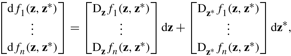

![$$\mathrm {d}\mathbf {f}(\mathbf {z},{\mathbf {z}}^*)=[\mathrm {d}f_1^{\,} (\mathbf {z},{\mathbf {z}}^*), \ldots ,\mathrm {d}f_n^{\,} (\mathbf {z},{\mathbf {z}}^*)]^T$$](../images/492994_1_En_2_Chapter/492994_1_En_2_Chapter_TeX_IEq163.png) , while
, while 

![$$\mathbf {F} ( \mathbf {Z},{\mathbf {Z}}^*) = [{\mathbf {f}}_1^{\,} (\mathbf {Z},{\mathbf {Z}}^*),\ldots ,{\mathbf {f}}_q^{\,} (\mathbf {Z},{\mathbf {Z}}^*)]$$](../images/492994_1_En_2_Chapter/492994_1_En_2_Chapter_TeX_IEq164.png) , then
, then ![$$\mathrm {d}\mathbf {F}(\mathbf {Z},{\mathbf {Z}}^*) = [\mathrm {d}{\mathbf {f}}_1^{\,} (\mathbf {Z},{\mathbf {Z}}^*),\ldots ,\mathrm {d} {\mathbf {f}}_q^{\,} (\mathbf {Z},{\mathbf {Z}}^*)]$$](../images/492994_1_En_2_Chapter/492994_1_En_2_Chapter_TeX_IEq165.png) , and (2.3.47) holds for the vector functions
, and (2.3.47) holds for the vector functions  . This implies that
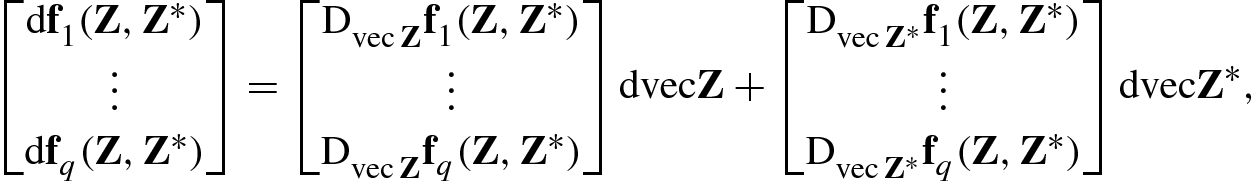
 and
and  .
.
![$$\displaystyle \begin{aligned} \mathrm{d} \mathrm{vec} \mathbf{Z}&=[\mathrm{d}Z_{11},\ldots ,\mathrm{d} Z_{m1},\ldots ,\mathrm{d}Z_{1n},\ldots ,\mathrm{d}Z_{mn}]^T,\\ \mathrm{d} \mathrm{vec} {\mathbf{Z}}^*&=[\mathrm{d}Z_{11}^*,\ldots ,\mathrm{d}Z_{m1}^*, \ldots ,\mathrm{d}Z_{1n}^*,\ldots ,\mathrm{d}Z_{mn}^*]^T,\\ \mathrm{d} \mathrm{vec} \mathbf{F}(\mathbf{Z},{\mathbf{Z}}^*))&=[\mathrm{d}f_{11}(\mathbf{Z},{\mathbf{Z}}^*),\ldots , \mathrm{d}f_{p1}(\mathbf{Z}, {\mathbf{Z}}^*), \ldots ,\mathrm{d}f_{1q}(\mathbf{Z}, {\mathbf{Z}}^*),\\ & \qquad \ldots ,\mathrm{d}f_{pq}(\mathbf{Z},{\mathbf{Z}}^*)]^T, \end{aligned} $$](../images/492994_1_En_2_Chapter/492994_1_En_2_Chapter_TeX_Equaa.png)


 with
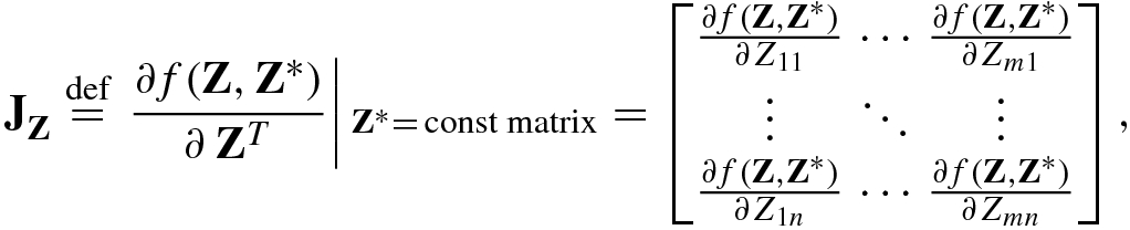
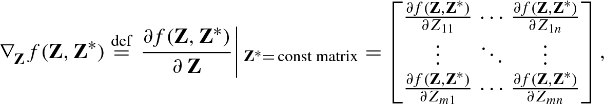
with
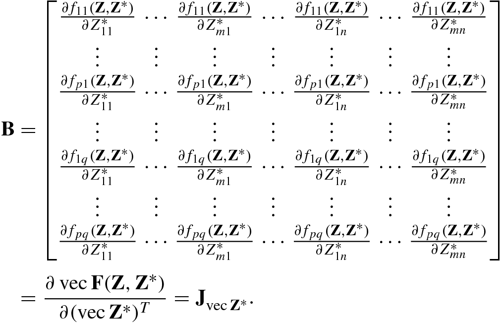
 , we have its complex Jacobian matrix and the complex gradient matrix:


 . By Proposition 2.3, the following identification formula is obtained:
The above equation shows that, as in the vector case, the key to identifying the gradient matrix and conjugate gradient matrix of a matrix function F(Z, Z ∗) is to write its matrix differential into the canonical form dF(Z, Z ∗) = A(dZ)TB + C(dZ ∗)TD.
 .
. Complex matrix differential and complex Jacobian matrix
Function | Matrix differential | Jacobian matrix |
|---|---|---|
f(z, z ∗) | df(z, z ∗) = adz + bdz ∗ |
|
f(z, z ∗) | df(z, z ∗) = a Tdz + b Tdz ∗ |
|
f(Z, Z ∗) | df(Z, Z ∗) = tr(AdZ + BdZ ∗) |
|
F(Z, Z ∗) | d vecF = Ad vecZ + Bd vecZ ∗ |
|
dF = A(dZ)B + C(dZ ∗)D |
| |
dF = A(dZ)TB + C(dZ ∗)TD |
|


This chapter presents the matrix differential for real and complex matrix functions. The matrix differential is a powerful tool for finding the gradient vectors/matrices that are key for update in optimization, as will see in the next chapter.