One of the most common problems in science and engineering is to solve the matrix equation Ax = b for finding x when the data matrix A and the data vector b are given.
- 1.
Well-determined equation: If m = n and rank(A) = n, i.e., the matrix A is nonsingular, then the matrix equation Ax = b is said to be well-determined.
- 2.
Under-determined equation: The matrix equation Ax = b is under-determined if the number of linearly independent equations is less than the number of independent unknowns.
- 3.
Over-determined equation: The matrix equation Ax = b is known as over-determined if the number of linearly independent equations is larger than the number of independent unknowns.
This chapter is devoted to describe singular value decomposition (SVD) together with Gauss elimination and conjugate gradient methods for solving well-determined matrix equations followed by Tikhonov regularization and total least squares for solving over-determined matrix equations, and the Lasso and LARS methods for solving under-determined matrix equations.
4.1 Gauss Elimination
First consider solution of well-determined equations. In well-determined equation, the number of independent equations and the number of independent unknowns are the same so that the solution of this system of equations is uniquely determined. The exact solution of a well-determined matrix equation Ax = b is given by x = A −1b. A well-determined equation is a consistent equation.
In this section, we deal with Gauss elimination method and conjugate gradient methods for solving an over-determined matrix equation Ax = b and finding the inverse of a singular matrix. This method performs only elementary row operations to the augmented matrix B = [A, b].
4.1.1 Elementary Row Operations
When solving an m × n system of linear equations, it is useful to reduce equations. The principle of reduction processes is to keep the solutions of the linear systems unchanged.
Two linear systems of equations in n unknowns are said to be equivalent systems if they have the same sets of solutions.
To transform a given m × n matrix equation A m×nx n = b m into an equivalent system, a simple and efficient way is to apply a sequence of elementary operations on the given matrix equation.
Type I: Interchange any two equations, say the pth and qth equations; this is denoted by R p ↔ R q.
Type II: Multiply the pth equation by a nonzero number α; this is denoted by αR p → R p.
Type III: Add β times the pth equation to the qth equation; this is denoted by βR p + R q → R q.
Clearly, any above type of elementary row operation does not change the solution of a system of linear equations, so after elementary row operations, the reduced system of linear equations and the original system of linear equations are equivalent.
The leftmost nonzero entry of a nonzero row is called the leading entry of the row. If the leading entry is equal to 1 then it is said to be the leading-1 entry.
As a matter of fact, any elementary operation on an m × n system of equations Ax = b is equivalent to the same type of elementary operation on the augmented matrix B = [A, b], where the column vector b is written alongside A. Therefore, performing elementary row operations on a system of linear equations Ax = b can be in practice implemented by using the same elementary row operations on the augmented matrix B = [A, b].
The discussions above show that if, after a sequence of elementary row operations, the augmented matrix B m×(n+1) becomes another simpler matrix C m×(n+1) then two matrices are row equivalent for the same solution of linear system.
For the convenience of solving a system of linear equations, the final row equivalent matrix should be of echelon form.
all rows with all entries zero are located at the bottom of the matrix;
the leading entry of each nonzero row appears always to the right of the leading entry of the nonzero row above;
all entries below the leading entry of the same column are equal to zero.
An echelon matrix B is said to be a reduced row-echelon form (RREF) matrix if the leading entry of each nonzero row is a leading-1 entry, and each leading-1 entry is the only nonzero entry in the column in which it is located.
Any m × n matrix A is row equivalent to one and only one matrix in reduced row-echelon form.
See [27, Appendix A].
A pivot position of an m × n matrix A is the position of some leading entry of its echelon form. Each column containing a pivot position is called a pivot column of the matrix A.
4.1.2 Gauss Elimination for Solving Matrix Equations
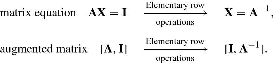
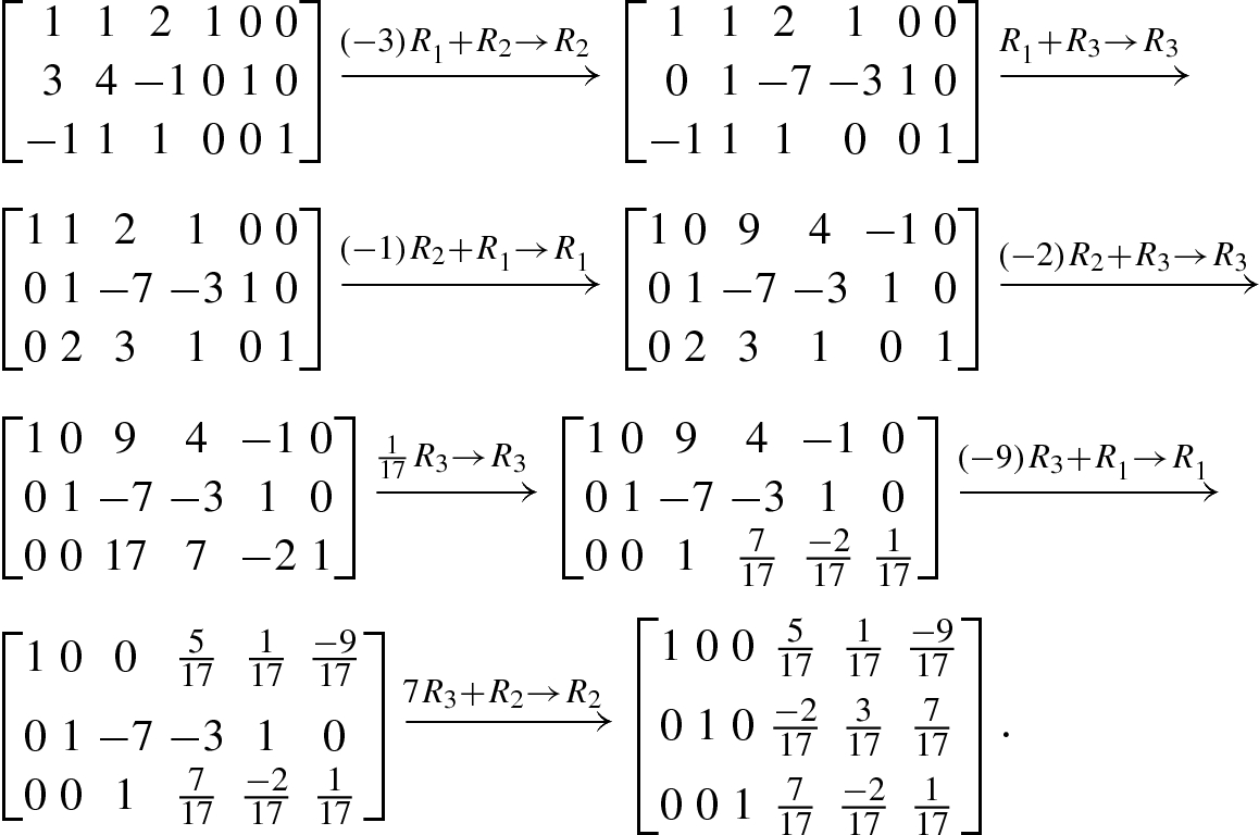
Elementary row operations can be used to solve matrix equations and perform matrix inversion.
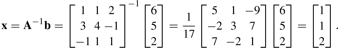
Consider how to solve an n × n matrix equation Ax = b, where the inverse matrix A −1 of the matrix A exists. We hope that the solution vector x = A −1b can be obtained by using elementary row operations.


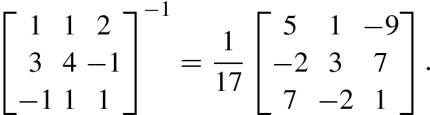
4.1.3 Gauss Elimination for Matrix Inversion


4.2 Conjugate Gradient Methods
 is a nonsingular matrix. This matrix equation can be equivalently written as


An iteration in the form of Eq. (4.2.3) is termed as a stationary iterative method and is not as effective as a nonstationary iterative method.
 is related to the former iteration solutions
  . The most typical nonstationary iteration method is the Krylov subspace method, described by


 is the initial iteration value and
  denotes the initial residual vector.
Krylov subspace methods have various forms, of which the three most common are the conjugate gradient method, the biconjugate gradient method, and the preconditioned conjugate gradient method.
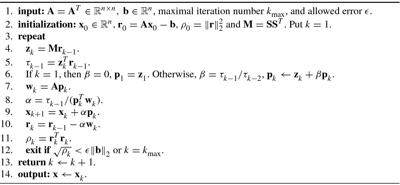
4.2.1 Conjugate Gradient Algorithm
The conjugate gradient method uses  as the initial residual vector. The applicable object of the conjugate gradient method is limited to the symmetric positive definite equation, Ax = b, where A is an n × n symmetric positive definite matrix.
 is said to be A-orthogonal or A-conjugate if
This property is known as A-orthogonality or A-conjugacy. Obviously, if A = I, then the A-conjugacy reduces to general orthogonality.
All algorithms adopting the conjugate vector as the update direction are known as conjugate direction algorithms. If the conjugate vectors  are not predetermined, but are updated by the gradient descent method in the updating process, then we say that the minimization algorithm for the objective function f(x) is a conjugate gradient algorithm.
Algorithm 4.1 gives a conjugate gradient algorithm.
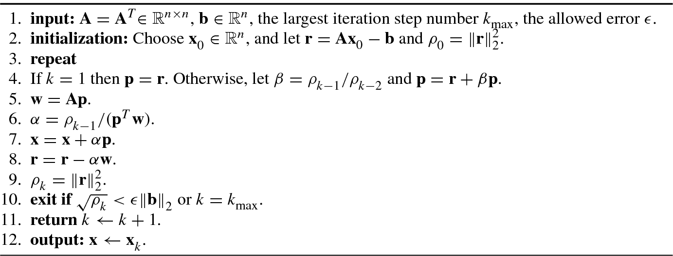


The fixed-iteration method requires the updating of the iteration matrix M, but no matrix needs to be updated in Algorithm 4.1. Hence, the Krylov subspace method is also called the matrix-free method [24].
4.2.2 Biconjugate Gradient Algorithm
 , that are A-conjugate in this method:
 are the residual vectors associated with search directions p
i and
are the residual vectors associated with search directions p
i and  , respectively. Algorithm 4.2 shows a biconjugate gradient algorithm.
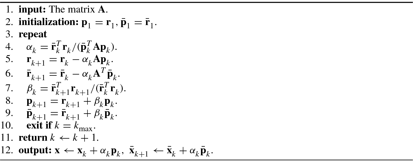
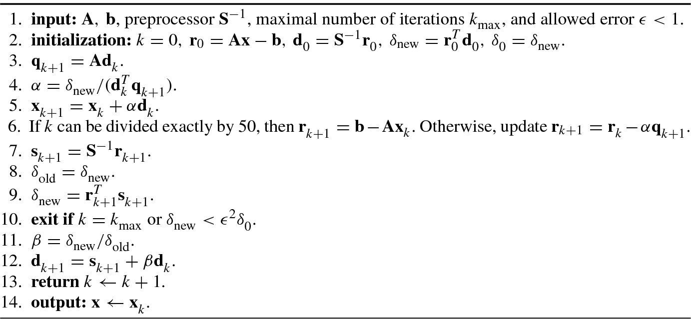
4.2.3 Preconditioned Conjugate Gradient Algorithm
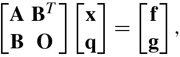
The basic idea of the preconditioned conjugate gradient iteration is as follows: through a clever choice of the scalar product form, the preconditioned saddle matrix becomes a symmetric positive definite matrix.
To simplify the discussion, we assume that the matrix equation with large condition number Ax = b needs to be converted into a new symmetric positive definite equation. To this end, let M be a symmetric positive definite matrix that can approximate the matrix A and for which it is easier to find the inverse matrix. Hence, the original matrix equation Ax = b is converted into M −1Ax = M −1b such that the new and original matrix equations have the same solution. However, in the new matrix equation M −1Ax = M −1b there is a hidden danger: M −1A is generally not either symmetric or positive definite even if both M and A are symmetric positive definite. Therefore, it is unreliable to use the matrix M −1 directly as the preprocessor of the matrix equation Ax = b.
 , then the preconditioned matrix equation is given by
Compared with the matrix M −1A, which is not symmetric positive definite, S −1AS −T must be symmetric positive definite if A is symmetric positive definite. The symmetry of S −1AS −T is easily seen, its positive definiteness can be verified as follows: by checking the quadratic function it easily follows that y T(S −1AS −T)y = z TAz, where z = S −Ty. Because A is symmetric positive definite, we have z TAz > 0, ∀ z ≠ 0, and thus y T(S −1AS −T)y > 0, ∀ y ≠ 0. That is to say, S −1AS −T must be positive definite.
At this point, the conjugate gradient method can be applied to solve the matrix equation (4.2.9) in order to get  , and then we can recover x via
  .
.
Algorithm 4.3 shows a preconditioned conjugate gradient (PCG) algorithm with a preprocessor, developed in [37].
 , as follows [24]:
A wonderful introduction to the conjugate gradient method is presented in [37].
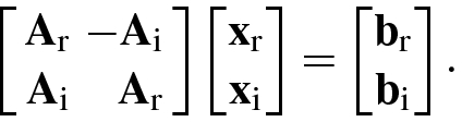
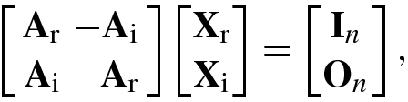
 , we can write it as the following real matrix equation:
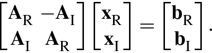
Clearly, if A = A
R + jA
I is a Hermitian positive definite matrix, then Eq. (4.2.10) is a symmetric positive definite matrix equation. Hence,  can be solved by adopting the conjugate gradient algorithm or the preconditioned conjugate gradient algorithm.
The main advantage of gradient methods is that the computation of each iteration is very simple; however, their convergence is generally slow.
4.3 Condition Number of Matrices
In many applications in science and engineering, it is often necessary to consider an important problem: there exist some uncertainties or errors in the actual observation data, and, furthermore, numerical calculation of the data is always accompanied by error. What is the impact of these errors? Is a particular algorithm numerically stable for data processing?
the numerical stability of various kinds of algorithms;
the condition number or perturbation analysis of the problem of interest.
Given some application problem f where d ∗∈ D is the data without noise or disturbance in a data group D. Let f(d ∗) ∈ F denote the solution of f, where F is a solution set. For observed data d ∈ D, we want to evaluate f(d). Owing to background noise and/or observation error, f(d) is usually different from f(d ∗). If f(d) is “close” to f(d ∗), then the problem f is said to be a “well-conditioned problem.” On the contrary, if f(d) is obviously different from f(d ∗) even when d is very close to d ∗, then we say that the problem f is an “ill-conditioned problem.” If there is no further information about the problem f, the term “approximation” cannot describe the situation accurately.
In perturbation theory, a method or algorithm for solving a problem f is said to be numerically stable if its sensitivity to a perturbation is not larger than the sensitivity inherent in the original problem. More precisely, f is stable if the approximate solution f(d) is close to the solution f(d ∗) without perturbation for all d ∈ D close to d ∗.
To mathematically describe numerical stability of a method or algorithm, we first consider the well-determined linear equation Ax = b, where the n × n coefficient matrix A has known entries and the n × 1 data vector b is also known, while the n × 1 vector x is an unknown parameter vector to be solved. Naturally, we are interested in the numerical stability of this solution: if the coefficient matrix A and/or the data vector b are perturbed, how will the solution vector x be changed? Does it maintain a certain stability? By studying the influence of perturbations of the coefficient matrix A and/or the data vector b, we can obtain a numerical value, called the condition number, describing an important characteristic of the coefficient matrix A.


![$$\displaystyle \begin{aligned} \delta\mathbf{x} &=\big ((\mathbf{A}+\delta \mathbf{A})^{-1}-{\mathbf{A}}^{-1}\big )\mathbf{b} \\ &= \big [{\mathbf{A}}^{-1}\big ( \mathbf{A}-(\mathbf{A}+\delta\mathbf{A})\big )(\mathbf{A}+\delta\mathbf{A})^{-1}\big ]\mathbf{b}\\ &=-{\mathbf{A}}^{-1} \delta\mathbf{A}(\mathbf{A}+\delta \mathbf{A})^{-1}\mathbf{b} \\ &=-{\mathbf{A}}^{-1} \delta\mathbf{A}(\mathbf{x}+\delta\mathbf{x}). \end{aligned} $$](../images/492994_1_En_4_Chapter/492994_1_En_4_Chapter_TeX_Equ21.png)


cond(A) = cond(A −1).
cond(cA) = cond(A).
cond(A) ≥ 1.
cond(AB) ≤cond(A)cond(B).

An orthogonal matrix A is perfectly conditioned in the sense that cond(A) = 1.
- ℓ 1 condition number, denoted as cond1(A), is defined as
 (4.3.9)
 - ℓ 2 condition number, denoted as cond2(A), is defined aswhere
 (4.3.10)
 and
and  are the maximum and minimum eigenvalues of A
HA, respectively; and
are the maximum and minimum eigenvalues of A
HA, respectively; and  and
and  are the maximum and minimum singular values of A, respectively.
 - ℓ ∞condition number, denoted as cond∞(A), is defined as
 (4.3.11)
 - Frobenius norm condition number, denoted as condF(A), is defined as
 (4.3.12)

 .
.It should be noticed that when using the LS method to solve the matrix equation Ax = b, a matrix A with a larger condition number may result into a worse solution due to cond2(A HA) = (cond2(A))2.

On the more effective methods than QR factorization for solving over-determined matrix equations, we will discuss them after introducing the singular value decomposition.
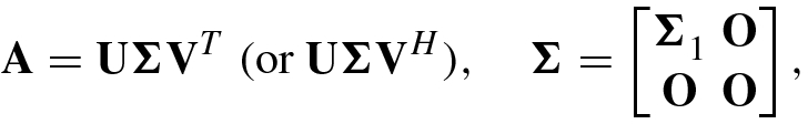
4.4 Singular Value Decomposition (SVD)
Beltrami (1835–1899) and Jordan (1838–1921) are recognized as the founders of singular value decomposition (SVD): Beltrami in 1873 published the first paper on SVD [2]. One year later, Jordan published his own independent derivation of SVD [23].
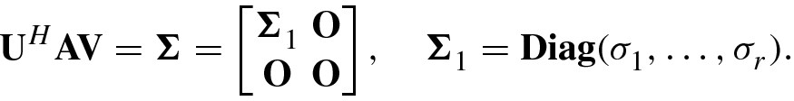
4.4.1 Singular Value Decomposition
 (or
(or
 ), then there exist orthogonal (or unitary) matrices
 (or
(or
 ) and
) and
 (or
(or
 ) such that
![$$\mathbf {U}=[{\mathbf {u}}_1,\ldots ,{\mathbf {u}}_m]\in \mathbb {C}^{m\times m}, \mathbf {V}=[{\mathbf {v}}_1,\ldots ,\mathbf { v}_n]\in \mathbb {C}^{n\times n}$$](../images/492994_1_En_4_Chapter/492994_1_En_4_Chapter_TeX_IEq29.png) and
and
 with diagonal entries

in which  and r = rank of A.
This theorem was first shown by Eckart and Young [11] in 1939, but the proof by Klema and Laub [26] is simpler.
The nonzero values  together with the zero values
  are called the singular values of the matrix A, and u
1, …, u
m and v
1, …, v
n are known as the left- and right singular vectors, respectively, while
are called the singular values of the matrix A, and u
1, …, u
m and v
1, …, v
n are known as the left- and right singular vectors, respectively, while  and
and  are called the left- and right singular vector matrices, respectively.
- 1.The SVD of a matrix A can be rewritten as the vector form
 (4.4.3)
This expression is sometimes said to be the dyadic decomposition of A [16].
- 2.Suppose that the n × n matrix V is unitary. Postmultiply (4.4.1) by V to get AV = U Σ, whose column vectors are given by
 (4.4.4)
 - 3.Suppose that the m × m matrix U is unitary. Premultiply (4.4.1) by U H to yield U HA = ΣV, whose column vectors are given by
 (4.4.5)
 - 4.
where
![$${\mathbf {U}}_r^{\,} =[{\mathbf {u}}_1^{\,} ,\ldots ,{\mathbf {u}}_r^{\,} ],{\mathbf {V}}_r^{\,} =[{\mathbf {v}}_1^{\,} ,\ldots ,{\mathbf {v}}_r^{\,} ]$$](../images/492994_1_En_4_Chapter/492994_1_En_4_Chapter_TeX_IEq39.png) , and
, and  . Equation (4.4.6) is called the truncated singular value decomposition or the thin singular value decomposition of the matrix A. In contrast, Eq. (4.4.1) is known as the full singular value decomposition.
- 5.which can be written in matrix form as
 (4.4.8)
Equations (4.4.1) and (4.4.8) are two definitive forms of SVD.
- 6.
From (4.4.1) it follows that AA H = U Σ 2U H. This shows that the singular value
 of an m × n matrix A is the positive square root of the corresponding nonnegative eigenvalue of the matrix product AA
H.
of an m × n matrix A is the positive square root of the corresponding nonnegative eigenvalue of the matrix product AA
H. - 7.If the matrix
 has rank r, then
 the leftmost r columns of the m × m unitary matrix U constitute an orthonormal basis of the column space of the matrix A, i.e.,
 ;
;the leftmost r columns of the n × n unitary matrix V constitute an orthonormal basis of the row space of A or the column space of A H, i.e.,
 ;
;the rightmost n − r columns of V constitute an orthonormal basis of the null space of the matrix A, i.e.,
 ;
;the rightmost m − r columns of U constitute an orthonormal basis of the null space of the matrix A H, i.e.,
 .
.


4.4.2 Properties of Singular Values
 are given by


 such that

The Eckart–Young theorem shows that the singular value  is equal to the minimum spectral norm of the error matrix E
k such that the rank of A + E
k is k − 1.
is equal to the minimum spectral norm of the error matrix E
k such that the rank of A + E
k is k − 1.
An important application of the Eckart–Young theorem is to the best rank-k approximation of the matrix A, where k < r = rank(A).


 , where
  . If the p × q matrix B is a submatrix of A with singular values
  , then

This is the interlacing theorem for singular values.
- 1.Relationship between Singular Values and Norms:

- 2.Relationship between Singular Values and Determinant:
 (4.4.16)
If all the
 are nonzero, then
  , which shows that A is nonsingular. If there is at least one singular value
  , then
  , namely A is singular. This is the reason why the
  are known as the singular values.
 - 3.Relationship between Singular Values and Condition Number:
 (4.4.17)
4.4.3 Singular Value Thresholding
 :
: 
 ,
,  .
.


If the soft threshold value τ = 0, then the SVT is reduced to the truncated SVD (4.4.18).
All of singular values are soft thresholded by the soft threshold value τ > 0, which just changes the magnitudes of singular values, does not change the left and right singular vector matrices U and V.
 , the SVT operator obeys

![$$\displaystyle \begin{aligned}{}[\mathrm{soft}(\mathbf{W},\mu )]_{ij}=\left\{\begin{aligned} &w_{ij}^{\,} -\mu ,&&~~w_{ij}^{\,} >\mu ;\\ &w_{ij}^{\,} +\mu ,&&~~w_{ij}^{\,} <-\mu ;\\ &0,&&~~\mathrm{otherwise}.\end{aligned}\right. \end{aligned} $$](../images/492994_1_En_4_Chapter/492994_1_En_4_Chapter_TeX_Equ52.png)
Here  is the (i, j)th entry of
  .
.
4.5 Least Squares Method
In over-determined equation, the number of independent equations is larger than the number of independent unknowns, the number of independent equations appears surplus for determining the unique solution. An over-determined matrix equation Ax = b has no exact solution and thus is an inconsistent equation that may in some cases have an approximate solution. There are four commonly used methods for solutions of matrix equations: Least squares method, Tikhonov regularization method, Gauss–Seidel method, and total least squares method. From this section we will introduce these four methods in turn.
4.5.1 Least Squares Solution
Consider an over-determined matrix equation Ax = b, where b is an m × 1 data vector, A is an m × n data matrix, and m > n.
Suppose the data vector and the additive observation error or noise exist, i.e., b = b 0 + e, where b 0 and e are the errorless data vector and the additive error vector, respectively.

 is minimized, namely


- Identifiable: When Ax = b is the over-determined equation, it has the unique solutionor
 (4.5.4)where B † denotes the Moore–Penrose inverse matrix of B. In parameter estimation theory, the unknown parameter vector x is said to be uniquely identifiable, if it is uniquely determined.
 (4.5.5)
 Unidentifiable: For an under-determined equation Ax = b, if rank(A) = m < n, then different solutions of x give the same value of Ax. Clearly, although the data vector b can provide some information about Ax, we cannot distinguish different parameter vectors x corresponding to the same Ax. Such an unknown vector x is said to be unidentifiable.
In parameter estimation, an estimate  of the parameter vector θ is known as an unbiased estimator, if its mathematical expectation is equal to the true unknown parameter vector, i.e.,
  . Further, an unbiased estimator is called the optimal unbiased estimator if it has the minimum variance. Similarly, for an over-determined matrix equation Aθ = b + e with noisy data vector b, if the mathematical expectation of the LS solution
  is equal to the true parameter vector θ, i.e.,
  , then
  is called the optimal unbiased estimator.

![$$\mathbf {e}=[e_1^{\,} ,\cdots ,e_m^{\,} ]^T$$](../images/492994_1_En_4_Chapter/492994_1_En_4_Chapter_TeX_IEq72.png) , and its mean vector and covariance matrix are, respectively,
, and its mean vector and covariance matrix are, respectively, 
 , if and only if rank(A) = n. In this case, the optimal unbiased solution is given by the LS solution

where  is any other solution of the matrix equation Ax = b + e.
See e.g., [46].
In the Gauss–Markov theorem cov(e) = σ 2I implies that all components of the additive noise vector e are mutually uncorrelated, and have the same variance σ 2. Only in this case, the LS solution is unbiased and optimal.
4.5.2 Rank-Deficient Least Squares Solutions
In many science and engineering applications, it is usually necessary to use a low-rank matrix to approximate a noisy or disturbed matrix. The following theorem gives an evaluation of the quality of approximation.
 be the SVD of
  , where p = rank(A). If k < p and
  is the rank-k approximation of A, then the approximation quality can be measured by the Frobenius norm

 . The LS solution
 .
.
![$$\displaystyle \begin{aligned} r_{\mathrm{LS}}^{\,}=\| \mathbf{Ax}_{\mathrm{LS}}^{\,}-\mathbf{b} \|{}_2^{\,} =\big\| [{\mathbf{u}}_{r+1}^{\,}, \ldots , {\mathbf{u}}_m^{\,} ]^H \mathbf{b} \big\|{}_2^{\,}.{} \end{aligned} $$](../images/492994_1_En_4_Chapter/492994_1_En_4_Chapter_TeX_Equ64.png)
Although, in theory, when i > r the true singular values  , the computed singular values
  , are not usually equal to zero and sometimes even have quite a large perturbation. In these cases, an estimate of the matrix rank r is required. In signal processing and system theory, the rank estimate
  is usually called the effective rank.
- 1.Normalized Singular Value Method. Compute the normalized singular values
 , and select the largest integer i satisfying the criterion
  as an estimate of the effective rank
  . Obviously, this criterion is equivalent to choosing the maximum integer i satisfying
 (4.5.13)
as
 ; here 𝜖 is a very small positive number, e.g., 𝜖 = 0.1 or 𝜖 = 0.05.
 - 2.Norm Ratio Method. Let an m × n matrix
 be the rank-k approximation to the original m × n matrix A. Define the Frobenius norm ratio as
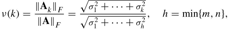 (4.5.14)and choose the minimum integer k satisfying
 (4.5.15)
as the effective rank estimate
 , where α is close to 1, e.g., α = 0.997 or 0.998.
 is determined via the above two criteria,
 .
.4.6 Tikhonov Regularization and Gauss–Seidel Method
The LS method is widely used for solving matrix equations and is applicable for many real-world applications in machine learning, neural networks, support vector machines, and evolutionary computation. But, due to its sensitive to the perturbation of the data matrix, the LS methods must be improved in these applications. A simple and efficient way is the well-known Tikhonov regularization.
4.6.1 Tikhonov Regularization
When m = n, and A is nonsingular, the solution of matrix equation Ax = b is given by  ; and when m > n and A
m×n is of full column rank, the solution of the matrix equation is
; and when m > n and A
m×n is of full column rank, the solution of the matrix equation is  .
.
The problem is: the data matrix A is often rank deficient in engineering applications. In these cases, the solution  or
or  either diverges, or even exists, it is the bad approximation to the unknown vector x. Even if we happen to find a reasonable approximation of x, the error estimate
  or
or  is very disappointing [32]. By observation, it is easily known that the problem lies in the inversion of the covariance matrix A
HA of the rank-deficient data matrix A.
is very disappointing [32]. By observation, it is easily known that the problem lies in the inversion of the covariance matrix A
HA of the rank-deficient data matrix A.
 , Tikhonov [39] in 1963 proposed the regularized least squares cost function


 , then the Tikhonov regularization solution

The nature of Tikhonov regularization method is: by adding a very small disturbance λ to each diagonal entry of the covariance matrix A HA of rank-deficient matrix A, the inversion of the singular covariance matrix A HA becomes the inversion of a nonsingular matrix A HA + λI, thereby greatly improving the numerical stability of solving the rank-deficient matrix equation Ax = b.

When the regularization parameter λ varies in the definition interval [0, ∞), the family of solutions for a regularized LS problem is known as its regularization path.
- 1.
Linearity: The Tikhonov regularization LS solution
 is the linear function of the observed data vector b.
 - 2.Limit characteristic when λ → 0: When the regularization parameter λ → 0, the Tikhonov regularization LS solution converges to the ordinary LS solution or the Moore–Penrose solution
 . The solution point
  has the minimum
  -norm among all the feasible points meeting A
H(Ax −b) = 0:
-norm among all the feasible points meeting A
H(Ax −b) = 0:  (4.6.4)
 - 3.
Limit characteristic when λ →∞: When λ →∞, the optimal Tikhonov regularization LS solution converges to a zero vector, i.e.,
 .
. - 4.
Regularization path: When the regularization parameter λ varies in [0, ∞), the optimal solution of the Tikhonov regularization LS problem is the smooth function of the regularization parameter, i.e., when λ decreases to zero, the optimal solution converges to the Moore–Penrose solution; and when λ increases, the optimal solution converges to zero vector.
The Tikhonov regularization can effectively prevent the divergence of the LS solution  when A is rank deficient, thereby improves obviously the convergence property of the LS algorithm and the alternative LS algorithm, and is widely applied.
4.6.2 Gauss–Seidel Method


![$${\mathbf {x}}^{(1)}=\big [x_1^{(1)},\ldots ,x_n^{(1)}\big ]^T$$](../images/492994_1_En_4_Chapter/492994_1_En_4_Chapter_TeX_IEq105.png) , we then continue this same kind of iteration for x
(2), x
(3), … until x converges.
, we then continue this same kind of iteration for x
(2), x
(3), … until x converges.The Gauss–Seidel method not only can find the solution of the matrix equation, but also are applicable for solving a nonlinear optimization problem.
 be the feasible set of
  vector
  . Consider the nonlinear minimization problem
 is the Cartesian product of a closed nonempty convex set
  , and
, and  .
.Equation (4.6.7) is an unconstrained optimization problem with m coupled variable vectors. An efficient approach for solving this class of the coupled optimization problems is the block nonlinear Gauss–Seidel method, called simply the GS method [3, 18].
- 1.
Initial m − 1 variable vectors
 , and let k = 0.
 - 2.Find the solution of separated sub-optimization problem
 (4.6.8)
At the (k + 1)th iteration of updating
 , all
, all  have been updated as
  , so these sub-vectors and
  to be updated are fixed as the known vectors.
 - 3.
To test whether m variable vectors are all convergent. If convergent, then output the optimization results
 ; otherwise, let k ← k + 1, return to Eq. (4.6.8), and continue to iteration until the convergence criterion meets.
If the objective function f(x) of the optimization (4.6.7) is the LS error function (for example,  , then the GS method is customarily called the alternating least squares (ALS) method.


The fact that the GS algorithm may not converge was observed by Powell in 1973 [34] who called it the “circle phenomenon” of the GS method. Recently, a lot of simulation experiences have shown [28, 31] that even converged, the iterative process of the ALS method is also very easy to fall into the “swamp”: an unusually large number of iterations leads to a very slow convergence rate. [28, 31].

The above algorithm is called the proximal point versions of the GS methods [1, 3], abbreviated as PGS method.
The role of the regularization term  is to force the updated vector
  close to
  , not to deviate too much, and thus avoid the violent shock of the iterative process in order to prevent the divergence of the algorithm.
The GS or PGS method is said to be well defined, if each sub-optimization problem has an optimal solution [18].
If the PGS method is well defined, and the sequence {x
k} exists limit points, then every limit point  of {x
k} is a critical point of the optimization problem (4.6.7).
of {x
k} is a critical point of the optimization problem (4.6.7).
This theorem shows that the convergence performance of the PGS method is better than that of the GS method.
Many simulation experiments show [28] that under the condition achieving the same error, the iterative number of the GS method in swamp iteration is unusually large, whereas the PGS method tends to converge quickly. The PGS method is also called the regularized Gauss–Seidel method in some literature.
The ALS method and the regularized ALS method have important applications in nonnegative matrix decomposition and the tensor analysis.
4.7 Total Least Squares Method
For a matrix equation A m×nx n = b m, all the LS method, the Tikhonov regularization method, and the Gauss–Seidel method give the solution of n parameters. However, by the rank-deficiency of the matrix A we know that the unknown parameter vector x contains only r independent parameters; the other parameters are linearly dependent on the r independent parameters. In many engineering applications, we naturally want to find the r independent parameters other than the n parameters containing redundancy components. In other words, we want to estimate only the principal parameters and to eliminate minor components. This problem can be solved via the low-rank total least squares (TLS) method.
The earliest ideas about TLS can be traced back to the paper of Pearson in 1901 [33] who considered the approximate method for solving the matrix equation Ax = b when both A and b exist the errors. But, only in 1980, Golub and Van Loan [15] have first time made the overall analysis from the point of view of numerical analysis, and have formally known this method as the total least squares. In mathematical statistics, this method is called the orthogonal regression or errors-in-variables regression [14]. In system identification, the TLS method is called the characteristic vector method or the Koopmans–Levin method [42]. Now, the TLS method has been widely used in statistics, physics, economics, biology and medicine, signal processing, automatic control, system science, artificial intelligence, and many other disciplines and fields.
4.7.1 Total Least Squares Solution


![$$\displaystyle \begin{aligned} \text{TLS:}\quad \min_{\Delta\mathbf{A},\Delta\mathbf{b},\mathbf{x}}\|[\Delta\mathbf{A},\Delta\mathbf{b}]\|{}_F^2\quad \text{subject to}\quad (\mathbf{A}+\Delta\mathbf{A})\mathbf{x}=\mathbf{b}+\Delta\mathbf{b} \end{aligned} $$](../images/492994_1_En_4_Chapter/492994_1_En_4_Chapter_TeX_Equ83.png)

 is the (n + 1) × 1 vector.
 and
and  , we have
  and thus can rewrite (4.7.4) as
 of B is significantly larger than
  , i.e., the smallest singular value has only one. In this case, the TLS problem (4.7.5) is easily solved via the Lagrange multiplier method. To this end, define the objective function
 , from
  it follows that
 of the matrix B
HB = [A, b]H[A, b] (i.e., the squares of the smallest singular value of B), while the TLS solution vector z is the eigenvector corresponding to the smallest eigenvalue
of the matrix B
HB = [A, b]H[A, b] (i.e., the squares of the smallest singular value of B), while the TLS solution vector z is the eigenvector corresponding to the smallest eigenvalue  of [A, b]H[A, b]. In other words, the TLS solution vector
  is the solution of the Rayleigh quotient minimization problem
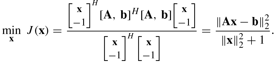
 , and their corresponding right singular vectors are
  . According to the above analysis, the TLS solution is
  , namely
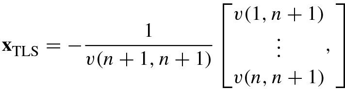

![$${\mathbf {V}}_1=[{\mathbf {v}}_{p+1}^{\,} ,{\mathbf {v}}_{p+2}^{\,} ,\cdots ,{\mathbf {v}}_{n+1}^{\,}]$$](../images/492994_1_En_4_Chapter/492994_1_En_4_Chapter_TeX_IEq137.png) will give n − p + 1 possible TLS solutions
will give n − p + 1 possible TLS solutions  . To find the unique TLS solution, one can make the Householder transformation Q to V
1 such that
. To find the unique TLS solution, one can make the Householder transformation Q to V
1 such that 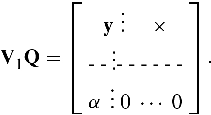
 . This algorithm was proposed by Golub and Van Loan [15], as shown in Algorithm 4.5.
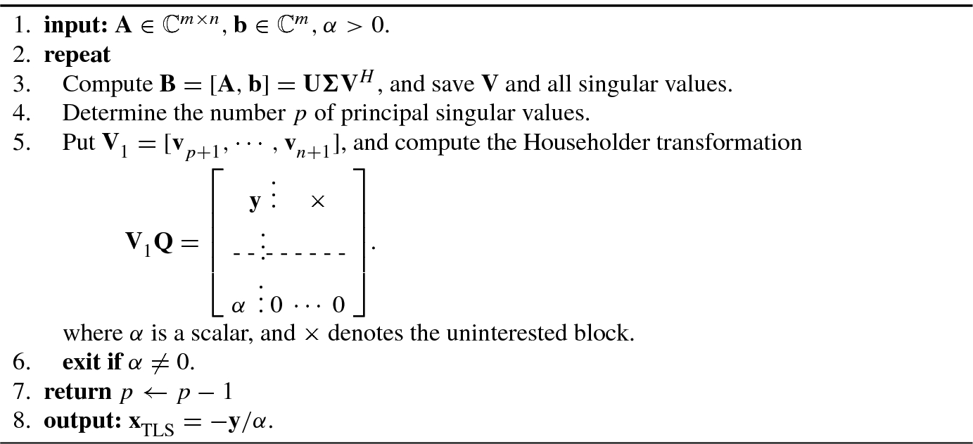
The above minimum norm solution  contains n parameters other than p independent principal parameters because of rank(A) = p < n.
 be an optimal approximation with rank p of the augmented matrix B, where
  . Denote the m × (p + 1) matrix
  as a submatrix among the m × (n + 1) optimal approximate matrix
  :
: 
 .
. , where x
(p) is the column vector consisting of p linearly independent unknown parameters of the vector x. Then, the original TLS problem becomes the solution of the following (n + 1 − p) TLS problems:
, where x
(p) is the column vector consisting of p linearly independent unknown parameters of the vector x. Then, the original TLS problem becomes the solution of the following (n + 1 − p) TLS problems: 

 is defined in (4.7.13). It is not difficult to show that
 is a windowed segment of the kth column vector of V, defined as
 ![$$\displaystyle \begin{aligned} {\mathbf{v}}_k^i =[v(i,k),v(i+1,k),\cdots ,v(i+p,k)]^T. {} \end{aligned} $$](../images/492994_1_En_4_Chapter/492994_1_En_4_Chapter_TeX_Equ97.png)
![$$\displaystyle \begin{aligned} f(\mathbf{a})=&\,[\hat {\mathbf{B}} (1:p+1)\mathbf{a}]^H \hat{\mathbf{B}}(1:p+1)\mathbf{a} +[\hat {\mathbf{B}} (2:p+2)\mathbf{a}]^H \hat{\mathbf{B}}(2:p+2)\mathbf{a}\\ &\, +\cdots +[\hat{\mathbf{B}}(n+1-p:n+1)\mathbf{a}]^H\hat{\mathbf{B}}(n+1-p:n+1)\mathbf{a} \\ =&\,{\mathbf{a}}^H \left [ \sum_{i=1}^{n+1-p} [\hat{\mathbf{B}}(i:p+i)]^H\hat{\mathbf{B}}(i:p+i) \right ] \mathbf{a}. \end{aligned} $$](../images/492994_1_En_4_Chapter/492994_1_En_4_Chapter_TeX_Equ98.png)
![$$\displaystyle \begin{aligned} {\mathbf{S}}^{(p)}=\sum_{i=1}^{n+1-p}[\hat{\mathbf{B}}(i:p+i)]^H \hat{\mathbf{B}}(i:p+i), {} \end{aligned} $$](../images/492994_1_En_4_Chapter/492994_1_En_4_Chapter_TeX_Equ99.png)

 as follows:
![$${\mathbf {e}}_1^{\,} =[1,0,\cdots ,0]^T$$](../images/492994_1_En_4_Chapter/492994_1_En_4_Chapter_TeX_IEq150.png) , and the constant α > 0 represents the error energy. From (4.7.19) and (4.7.16) we have
, and the constant α > 0 represents the error energy. From (4.7.19) and (4.7.16) we have 
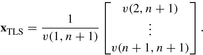
![$${\mathbf {x}}^{(p)}=[x_{\mathrm {TLS}}^{\,} (1),\cdots ,x_{\mathrm {TLS}}^{\,}(p)]^T$$](../images/492994_1_En_4_Chapter/492994_1_En_4_Chapter_TeX_IEq151.png) in the TLS solution vector
in the TLS solution vector  is given by

 , the low-rank SVD-TLS algorithm consists of the following steps [5].

4.7.2 Performances of TLS Solution
The TLS has two interesting explanations: one is its geometric interpretation [15], and another is its closed solution [43].
 be the ith row of the matrix A, and
  be the ith entry of the vector b. Then the TLS solution
  is the minimal vector such that
 is the distance from the point
  to the nearest point in the subspace
  , and the subspace
  is defined as
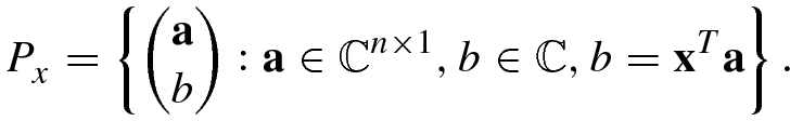
 [15]: the square sum of the distance from the TLS solution point
  to the subspace
  is minimized.
 , then the TLS solution can be expressed as [43]
 from the covariance matrix A
TA, and then finds the inverse matrix of
from the covariance matrix A
TA, and then finds the inverse matrix of  to get the LS solution.
 , then its covariance matrix
  . Obviously, when the error matrix E has zero mean, the mathematical expectation of the covariance matrix is given by
 of the (n + 1) × (n + 1) covariance matrix A
HA is the square of the singular value of the error matrix E. Because the square of singular value
of the (n + 1) × (n + 1) covariance matrix A
HA is the square of the singular value of the error matrix E. Because the square of singular value  happens to reflect the common variance σ
2 of each column vector of the error matrix, the covariance matrix
happens to reflect the common variance σ
2 of each column vector of the error matrix, the covariance matrix  of the error-free data matrix can be retrieved from
  , namely
  . In other words, the TLS method can effectively restrain the influence of the unknown error matrix.
It should be pointed out that the main difference between the TLS method and the Tikhonov regularization method for solving the matrix equation  is: the TLS solution can contain only p = rank([A, b]) principal parameters, and exclude the redundant parameters; whereas the Tikhonov regularization method can only provide all n parameters including redundant parameters.
4.7.3 Generalized Total Least Square
The ordinary LS, the Tikhonov regularization, and the TLS method can be derived and explained by a unified theoretical framework [46].
![$$\displaystyle \begin{aligned} \min_{\Delta \mathbf{A},\Delta\mathbf{b},\mathbf{x}} \left (\|[\Delta \mathbf{A},\Delta\mathbf{b}]\|{}_F^2 +\lambda \|\mathbf{x} \|{}_2^2\right ){} \end{aligned} $$](../images/492994_1_En_4_Chapter/492994_1_En_4_Chapter_TeX_Equ108.png)


 , then the above equation becomes
 ![$$\displaystyle \begin{aligned} \mathbf{Dz}=-\left [\alpha^{-1}\mathbf{A},\beta^{-1}\mathbf{b}\right ]\mathbf{z}. \end{aligned} $$](../images/492994_1_En_4_Chapter/492994_1_En_4_Chapter_TeX_Equ109.png)
![$$\displaystyle \begin{aligned} \min \|\mathbf{D}\|{}_F^2=\min\|\mathbf{D}\mathbf{z}\|{}_2^2=\min\big\|\big [\alpha^{-1}\mathbf{A},\beta^{-1}\mathbf{b}\big ]\mathbf{z}\big\|{}_2^2, \end{aligned}$$](../images/492994_1_En_4_Chapter/492994_1_En_4_Chapter_TeX_Equac.png)
![$$\displaystyle \begin{aligned} \hat{\mathbf{x}}_{\mathrm{GTLS}}^{\,} =\mathrm{arg}\min_{\mathbf{z}} \left (\frac{\|[\alpha^{-1}\mathbf{A},\beta^{-1}\mathbf{b}]\mathbf{z}\|{}_2^2}{\mathbf{ z}^H\mathbf{z}} +\lambda\|\mathbf{x}\|{}_2^2\right ).{} \end{aligned} $$](../images/492994_1_En_4_Chapter/492994_1_En_4_Chapter_TeX_Equ110.png)


- 1.Comparison of optimization problems
- The ordinary least squares: α = 0, β = 1 and λ = 0, which gives
 (4.7.32)
 - The Tikhonov regularization: α = 0, β = 1 and λ > 0, which gives
 (4.7.33)
 - The total least squares: α = β = 1 and λ = 0, which yields
 (4.7.34)
- 2.Comparison of solution vectors: When the weighting coefficients α, β and the Tikhonov regularization parameter λ take the suitable values, the GTLS solution (4.7.31) gives the following results:
 ,
, ,
, .
.
- 3.Comparison of perturbation methods
Ordinary LS method: it uses the possible small correction term Δb = Ax −b to disturb the data vector b such that b − Δb ≈b 0.
Tikhonov regularization method: it adds the same perturbation term λ > 0 to every diagonal entry of the matrix A HA for avoiding the numerical instability of the LS solution (A HA)−1A Hb.
TLS method: by subtracting the perturbation matrix λI, the noise or disturbance in the covariance matrix of the original data matrix is restrained.
- 4.Comparison of application ranges
The LS method is applicable for the data matrix A with full column rank and the data vector b existing the iid Gaussian errors.
The Tikhonov regularization method is applicable for the data matrix A with deficient column rank.
The TLS method is applicable for the data matrix A with full column rank and both A and the data vector b existing the iid Gaussian error.
4.8 Solution of Under-Determined Systems

4.8.1 ℓ 1-Norm Minimization
Can it ever be unique?
How to find the sparsest solution?

 -norm of an n × 1 vector x can be defined as
 denotes the number of all nonzero elements of x. Thus if
  , then x is sparse.
 -norm minimization

 .
. -norm minimization with the inequality constraint 𝜖 ≥ 0 which allows a certain error perturbation
A key term coined and defined in [9] that is crucial for the study of uniqueness is the sparsity of the matrix A.
Given a matrix A, its sparsity, denoted as σ = spark(A), is defined as the smallest possible number such that there exists a subgroup of σ columns from A that are linearly dependent.
The sparsity gives a simple criterion for uniqueness of sparse solution of an under-determined system of linear equations Ax = b, as stated below.
If a system of linear equations Ax = b has a solution x obeying ∥x∥0 < spark(A)∕2, this solution is necessarily the sparsest solution.
![$$\mathbf {x}=[x_i^{\,} ,\cdots ,x_n^{\,} ]^T$$](../images/492994_1_En_4_Chapter/492994_1_En_4_Chapter_TeX_IEq185.png) is called its support, denoted by
is called its support, denoted by  . The length of the support (i.e., the number of nonzero elements) is measured by
  -norm
-norm 
 is said to be K-sparse, if
  , where K ∈{1, ⋯ , n}.
 , then the vector
  is known as the K-sparse approximation.
 . Because ∥x∥p is the convex function if and only if p ≥ 1, the ℓ
1-norm is the objective function closest to ℓ
0-norm. Then, from the viewpoint of optimization, the ℓ
1-norm is said to be the convex relaxation of the ℓ
0-norm. Therefore, the ℓ
0-norm minimization problem (P
0) in (4.8.3) can transformed into the following convexly relaxed ℓ
1-norm minimization problem:
. Because ∥x∥p is the convex function if and only if p ≥ 1, the ℓ
1-norm is the objective function closest to ℓ
0-norm. Then, from the viewpoint of optimization, the ℓ
1-norm is said to be the convex relaxation of the ℓ
0-norm. Therefore, the ℓ
0-norm minimization problem (P
0) in (4.8.3) can transformed into the following convexly relaxed ℓ
1-norm minimization problem:

 -norm
-norm  , as the objective function, itself is the convex function, and the equality constraint b = Ax is the affine function.
The ℓ 1-norm minimization above is also called the basis pursuit (BP). This is a quadratically constrained linear programming (QCLP) problem.
 is the solution to (P
1), and
is the solution to (P
1), and  is the solution to (P
0), then [8]
is the solution to (P
0), then [8] 
 is only the feasible solution to (P
1), while
is only the feasible solution to (P
1), while  is the optimal solution to (P
1). The direct relationship between
is the optimal solution to (P
1). The direct relationship between  and
and  is given by
  .
. -norm minimization expression (4.8.4), the inequality
  -norm minimization expression (4.8.8) has also two variants:
 - Since x is constrained as K-sparse vector, the inequality ℓ 1-norm minimization becomes the inequality ℓ 2-norm minimizationThis is a quadratic programming (QP) problem.
 (4.8.10)
 - Using the Lagrange multiplier method, the inequality constrained ℓ 1-norm minimization problem (P 11) becomesThis optimization is called the basis pursuit denoising (BPDN) [7].
 (4.8.11)
The optimization problems (P
10) and (P
11) are, respectively, called the error constrained ℓ
1-norm minimization and ℓ
1-penalty minimization [41]. The  -penalty minimization is also known as the regularized
  linear programming or
  -norm regularization least squares.
 is minimized. That is to say, λ > 0 can balance the error squares sum cost function
  and the ℓ
1-norm cost function
and the ℓ
1-norm cost function  of the twin objectives
4.8.2 Lasso
The solution of a system of sparse equations is closely related to regression analysis. Minimizing the least squared error may usually lead to sensitive solutions. Many regularization methods were proposed to decrease this sensitivity. Among them, Tikhonov regularization [40] and Lasso [12, 38] are two widely known and cited algorithms, as pointed out in [44].
 and an observed data matrix
  , find a fitting coefficient vector
  such that


 is known as a predictor; and the vector x is simply called a coefficient vector.
 -norm of the prediction vector does not exceed an upper bound q, the squares sum of prediction errors is minimized, namely
The bound q is a tuning parameter. When q is large enough, the constraint has no effect on x and the solution is just the usual multiple linear least squares regression of x on  and
and  . However, for the smaller values of q (q ≥ 0), some of the coefficients
  will take zero. Choosing a suitable q will lead to a sparse coefficient vector x.

The Lasso problem involves both the  -norm constrained fitting for statistics and the data mining.
Contraction function: the Lasso shrinks the range of parameters to be estimated, only a small number of selected parameters are estimated at each step.
Selection function: the Lasso would automatically select a very small part of variables for linear regression, yielding a spare solution.
The Lasso method achieves the better prediction accuracy by shrinkage and variable selection.
The Lasso has many generalizations, here are a few examples. In machine learning, sparse kernel regression is referred to as the generalized Lasso [36]. Multidimensional shrinkage-thresholding method is known as the group Lasso [35]. A sparse multiview feature selection method via low-rank analysis is called the MRM-Lasso (multiview rank minimization-based Lasso) [45]. Distributed Lasso solves the distributed sparse linear regression problems [29].
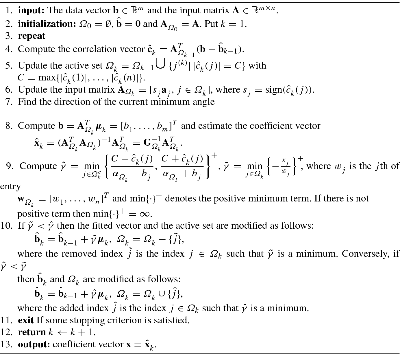
4.8.3 LARS
The LARS is the abbreviation of least angle regressions and is a stepwise regression method. Stepwise regression is also known as “forward stepwise regression.” Given a collection of possible predictors, X = {x 1, …, x m}, the aim of LARS is to identify the fitting vector most correlated with the response vector, i.e., the angle between the two vectors is minimized.
- 1.
The first step selects the fitting vector having largest absolute correlation with the response vector y, say
 , and performs simple linear regression of y on
  :
:  , where the residual vector r denotes the residuals of the remaining variables removing
  from X. The residual vector r is orthogonal to
  . When some predictors happen to be highly correlated with x
j and thus are approximately orthogonal to r, these predictors perhaps are eliminated, i.e., the residual vector r will not have information on these eliminating predictors.
. When some predictors happen to be highly correlated with x
j and thus are approximately orthogonal to r, these predictors perhaps are eliminated, i.e., the residual vector r will not have information on these eliminating predictors. - 2.
In the second step, r is regarded as the new response. The LARS selects the fitting vector having largest absolute correlation with the new response r, say
 , and performs simple linear regression
  . Repeat this selection process until no predictor has any correlation with r.
After k selection steps, one gets a set of predictors  that are then used in the usual way to construct a k-parameter linear model. This selection regression is an aggressive fitting technique that can be overly greedy [12]. The stepwise regression may be said to be of under-regression due to perhaps eliminating useful predictors that happen to be correlated with current predictor.
To avoid the under-regression in forward stepwise regression, the LARS algorithm allows “stagewise regression” to be implemented using fairly large steps.
Algorithm 4.6 shows the LARS algorithm developed in [12].
- 1.
Start with r = y and β 1 = β 2 = … = β p = 0.
- 2.
Find the predictor x j most correlated with r.
- 3.
Update β j ← β j + δ j, where
![$$\delta _j=\epsilon \cdot \mathrm {sign}[\mathrm {corr}(\mathbf {r},{\mathbf {x}}_j^{\,} )]$$](../images/492994_1_En_4_Chapter/492994_1_En_4_Chapter_TeX_IEq228.png) ;
; - 4.
Update r ←r − δ jx j, and repeat Steps 2 and 3 until no predictor has any correlation with r.
This chapter mainly introduces singular value decomposition and several typical methods for solving the well-determined, over-determined, and under-determined matrix equations.
Tikhonov regularization method and ℓ 1-norm minimization have wide applications in artificial intelligence.
Generalized total least squares method includes the LS method, Tikhonov regularization method, and total least squares method as special examples.
Algorithm 4.6 Least angle regressions (LARS) algorithm with Lasso modification [12]LAR algorithm