This chapter is devoted to another core subject of matrix algebra: the eigenvalue decomposition (EVD) of matrices, including various generalizations of EVD such as the generalized eigenvalue decomposition, the Rayleigh quotient, and the generalized Rayleigh quotient.
5.1 Eigenvalue Problem and Characteristic Equation
The eigenvalue problem not only is a very interesting theoretical problem but also has a wide range of applications in artificial intelligence.
5.1.1 Eigenvalue Problem
If ![$$\mathbb {L}[\mathbf {w}]=\mathbf {w}$$](../images/492994_1_En_5_Chapter/492994_1_En_5_Chapter_TeX_IEq1.png) holds for any nonzero vector w, then
holds for any nonzero vector w, then  is called an identity transformation. More generally, if, when a linear operator acts on a vector, the output is a multiple of this vector, then the linear operator is said to have an input reproducing characteristic.
 . If the output vector is the same as the input vector u up to a constant factor λ, i.e.,
 ![$$\displaystyle \begin{aligned} \mathbb{L}[\mathbf{u}]=\lambda \mathbf{u}, \quad \mathbf{u}\neq \mathbf{0},{} \end{aligned} $$](../images/492994_1_En_5_Chapter/492994_1_En_5_Chapter_TeX_Equ1.png)
 and the scalar λ is the corresponding eigenvalue of
  .
.
From the above definition, it is known that if each eigenvector u is regarded as an input of a linear time-invariant system  , then the eigenvalue λ associated with eigenvector u is equivalent to the gain of the linear system
  with u as the input. Only when the input of the system
  is an eigenvector u, its output is the same as the input up to a constant factor. Thus an eigenvector can be viewed as description of the characteristics of the system, and hence is also called a characteristic vector. This is a physical explanation of eigenvectors in relation to linear systems.
![$$\mathbb {L}[\mathbf {x}]=\mathbf {Ax}$$](../images/492994_1_En_5_Chapter/492994_1_En_5_Chapter_TeX_IEq9.png) , then its eigenvalue problem (5.1.1) can be written as
, then its eigenvalue problem (5.1.1) can be written as 
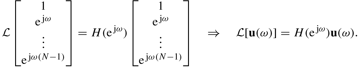
 . When inputting a complex exponential or harmonic signal ejωn, the system output is given by
 ![$$\displaystyle \begin{aligned}\mathbb{L}[\mathrm{e}^{\,\mathrm{j}\omega n}]=\sum_{k=-\infty}^\infty h(n-k)\mathrm{e}^{\,\mathrm{j}\omega k}=\sum_{k=-\infty}^\infty h(k)\mathrm{e}^{\,\mathrm{j}\omega (n-k)}=H(\mathrm{e}^{\,\mathrm{j}\omega})\mathrm{e}^{\,\mathrm{j}\omega n}. \end{aligned}$$](../images/492994_1_En_5_Chapter/492994_1_En_5_Chapter_TeX_Equa.png)
 is a Hermitian matrix then its eigenvalue λ must be a real number, and
![$$\mathbf {U}=[{\mathbf {u}}_1^{\,} ,\ldots ,{\mathbf {u}}_n^{\,}]^T$$](../images/492994_1_En_5_Chapter/492994_1_En_5_Chapter_TeX_IEq12.png) is a unitary matrix, and
is a unitary matrix, and  . Equation (5.1.3) is called the eigenvalue decomposition (EVD) of A.
Since an eigenvalue λ and its associated eigenvector u often appear in pairs, the two-tuple (λ, u) is called an eigenpair of the matrix A. An eigenvalue may take a zero value, but an eigenvector cannot be a zero vector.


Find all scalars λ (eigenvalues) such that the matrix |A − λI| = 0;
Given an eigenvalue λ, find all nonzero vectors u satisfying (A − λI)u = 0; they are the eigenvector(s) corresponding to the eigenvalue λ.
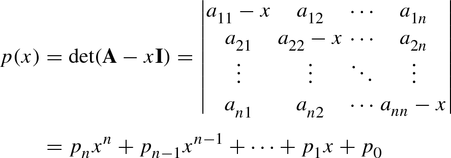
5.1.2 Characteristic Polynomial
 , i.e.,

The roots of the characteristic equation  are known as the eigenvalues, characteristic values, latent values, the characteristic roots, or latent roots.
Obviously, computing the n eigenvalues  of an n × n matrix A and finding the n roots of the nth-order characteristic polynomial
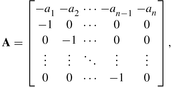
  are two equivalent problems. An n × n matrix A generates an nth-order characteristic polynomial. Likewise, each nth-order polynomial can also be written as the characteristic polynomial of an n × n matrix.

namely  .
.
5.2 Eigenvalues and Eigenvectors
Given an n × n matrix A, we consider the computation and properties of the eigenvalues and eigenvectors of A.
5.2.1 Eigenvalues
Even if an n × n matrix A is real, some roots of its characteristic equation may be complex, and the root multiplicity can be arbitrary or even equal to n. These roots are collectively referred to as the eigenvalues of the matrix A.
An eigenvalue λ of a matrix A is said to have algebraic multiplicity μ, if λ is a μ-multiple root of the characteristic polynomial  .
.
If the algebraic multiplicity of an eigenvalue λ is 1, then it is called a single eigenvalue. A nonsingle eigenvalue is said to be a multiple eigenvalue.

 , are not necessarily different from each other, and also are not necessarily real for a real matrix. For example, for the Givens rotation matrix
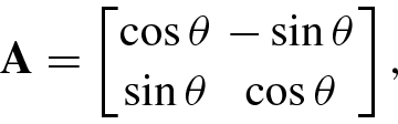

 . In this case, the characteristic equation cannot give a real value for λ, i.e., the two eigenvalues of the rotation matrix are complex, and the two corresponding eigenvectors are complex vectors.
- 1.
An n × n matrix A has a total of n eigenvalues, where multiple eigenvalues count according to their multiplicity.
- 2.
If a nonsymmetric real matrix A has complex eigenvalues and/or complex eigenvectors, then they must appear in the form of a complex conjugate pair.
- 3.
If A is a real symmetric matrix or a Hermitian matrix, then its all eigenvalues are real numbers.
- 4.The eigenvalues of a diagonal matrix and a triangular matrix satisfy the following:
if
 , then its eigenvalues are given by
 ;
;if A is a triangular matrix, then all its diagonal entries are eigenvalues.
- 5.Given an n × n matrix A:
if λ is an eigenvalue of A, then λ is also an eigenvalue of A T;
if λ is an eigenvalue of A, then λ ∗ is an eigenvalue of A H;
if λ is an eigenvalue of A, then λ + σ 2 is an eigenvalue of A + σ 2I;
if λ is an eigenvalue of A, then 1∕λ is an eigenvalue of its inverse matrix A −1.
- 6.
All eigenvalues of an idempotent matrix A 2 = A take 0 or 1.
- 7.
If A is an n × n real orthogonal matrix, then all its eigenvalues are located on the unit circle, i.e., |λ i(A)| = 1 for all i = 1, …, n.
- 8.The relationship between eigenvalues and the matrix singularity is as follows:
if A is singular, then it has at least one zero eigenvalue;
if A is nonsingular, then its all eigenvalues are nonzero.
- 9.
The relationship between eigenvalues and trace: the sum of all eigenvalues of A is equal to its trace, namely
 .
. - 10.
A Hermitian matrix A is positive definite (semidefinite) if and only if its all eigenvalues are positive (nonnegative).
- 11.
The relationship between eigenvalues and determinant: the product of all eigenvalues of A is equal to its determinant, namely
 .
. - 12.The Cayley–Hamilton theorem: if
 are the eigenvalues of an n × n matrix A, then
- 13.
If the n × n matrix B is nonsingular, then λ(B −1AB) = λ(A). If B is unitary, then λ(B HAB) = λ(A).
- 14.
The matrix products A m×nB n×m and B n×mA m×n have the same nonzero eigenvalues.
- 15.If an eigenvalue of a matrix A is λ, then the corresponding eigenvalue of the matrix polynomial
 is given by
  (5.2.2)
 - 16.
If λ is an eigenvalue of a matrix A, then eλ is an eigenvalue of the matrix exponential function eA.
5.2.2 Eigenvectors
 is a complex matrix, and λ is one of its eigenvalues, then the vector v satisfying

If a matrix A is Hermitian, then its all eigenvalues are real, and hence from Eq. (5.2.3) it is immediately known that ((A − λI)v)T = v T(A − λI) = 0 T, yielding v = u; namely, the right and left eigenvectors of any Hermitian matrix are the same.
The SVD is available for any m × n (where m ≥ n or m < n) matrix, while the EVD is available only for square matrices.
- For an n × n non-Hermitian matrix A, its kth singular value is defined as the spectral norm of the error matrix E k making the rank of the original matrix A decreased by 1:while its eigenvalues are defined as the roots of the characteristic polynomial
 (5.2.5)
 . There is no inherent relationship between the singular values and the eigenvalues of the same square matrix, but each nonzero singular value of an m × n matrix A is the positive square root of some nonzero eigenvalue of the n × n Hermitian matrix A
HA or the m × m Hermitian matrix AA
H.
. There is no inherent relationship between the singular values and the eigenvalues of the same square matrix, but each nonzero singular value of an m × n matrix A is the positive square root of some nonzero eigenvalue of the n × n Hermitian matrix A
HA or the m × m Hermitian matrix AA
H. The left singular vector
 and the right singular vector
  of an m × n matrix A associated with the singular value
  are defined as the two vectors satisfying
  , while the left and right eigenvectors are defined by
  and
and  , respectively. Hence, for the same n × n non-Hermitian matrix A, there is no inherent relationship between its (left and right) singular vectors and its (left and right) eigenvectors. However, the left singular vector
  and right singular vector
  of a matrix
  are, respectively, the eigenvectors of the m × m Hermitian matrix AA
H and of the n × n matrix A
HA.
are, respectively, the eigenvectors of the m × m Hermitian matrix AA
H and of the n × n matrix A
HA.
From Eq. (5.1.2) it is easily seen that after multiplying an eigenvector u of a matrix A by any nonzero scalar μ, then μu is still an eigenvector of A. In general it is assumed that eigenvectors have unit norm, i.e.,  .
.
Using eigenvectors we can introduce the condition number of any single eigenvalue.

 of a matrix
  is called the spectrum of the matrix A, denoted λ(A). The spectral radius of a matrix A, denoted ρ(A), is a nonnegative real number and is defined as
 , denoted In(A), is defined as the triplet
 are, respectively, the numbers of the positive, negative, and zero eigenvalues of A (each multiple eigenvalue is counted according to its multiplicity). Moreover, the quality i
+(A) − i
−(A) is known as the signature of A.
are, respectively, the numbers of the positive, negative, and zero eigenvalues of A (each multiple eigenvalue is counted according to its multiplicity). Moreover, the quality i
+(A) − i
−(A) is known as the signature of A.5.3 Generalized Eigenvalue Decomposition (GEVD)
The EVD of an n × n single matrix can be extended to the EVD of a matrix pair or pencil consisting of two matrices. The EVD of a matrix pencil is called the generalized eigenvalue decomposition (GEVD). As a matter of fact, the EVD is a special example of the GEVD.
5.3.1 Generalized Eigenvalue Decomposition
The basis of the EVD is the eigensystem expressed by the linear transformation ![$$\mathbb {L}[\mathbf {u}]=\lambda \mathbf {u}$$](../images/492994_1_En_5_Chapter/492994_1_En_5_Chapter_TeX_IEq45.png) : taking the linear transformation
: taking the linear transformation ![$$\mathbb {L}[\mathbf {u}]=\mathbf {Au}$$](../images/492994_1_En_5_Chapter/492994_1_En_5_Chapter_TeX_IEq46.png) , one gets the EVD Au = λu.
, one gets the EVD Au = λu.
 and
and  both of whose inputs are the vector u, but the output
 ![$$\mathbb {L}_a [\mathbf {u}]$$](../images/492994_1_En_5_Chapter/492994_1_En_5_Chapter_TeX_IEq49.png) of the first system
of the first system  is some constant times λ the output
 ![$$\mathbb {L}_b^{\,} [\mathbf {u}]$$](../images/492994_1_En_5_Chapter/492994_1_En_5_Chapter_TeX_IEq51.png) of the second system
of the second system  . Hence the eigensystem is generalized as [11]
![$$\displaystyle \begin{aligned} \mathbb{L}_a [\mathbf{u}]=\lambda\mathbb{L}_b^{\,} [\mathbf{u}]\quad (\mathbf{u}\neq \mathbf{0}); \end{aligned} $$](../images/492994_1_En_5_Chapter/492994_1_En_5_Chapter_TeX_Equ16.png)
 . The constant λ and the nonzero vector u are known as the generalized eigenvalue and the generalized eigenvector of generalized eigensystem
  , respectively.
![$$\mathbb {L}_a [\mathbf {u}]=\mathbf {Au}$$](../images/492994_1_En_5_Chapter/492994_1_En_5_Chapter_TeX_IEq55.png) and
and ![$$\mathbb {L}_b[\mathbf {u}]=\mathbf {Bu}$$](../images/492994_1_En_5_Chapter/492994_1_En_5_Chapter_TeX_IEq56.png) , then the generalized eigensystem becomes the generalized eigenvalue decomposition (GEVD):
, then the generalized eigensystem becomes the generalized eigenvalue decomposition (GEVD):

A generalized eigenvalue and its corresponding generalized eigenvector are collectively called a generalized eigenpair, denoted (λ, u). Equation (5.3.2) shows that the ordinary eigenvalue problem is a special example of the generalized eigenvalue problem when the matrix pencil is (A, I).

 is called the generalized characteristic polynomial of the matrix pencil (A, B), and
  is known as the generalized characteristic equation of the matrix pencil (A, B). Hence, the matrix pencil (A, B) is often expressed as A − λB.
The generalized eigenvalues of the matrix pencil (A, B) are all solutions z of the generalized characteristic equation  , including the generalized eigenvalues equal to zero. If the matrix B = I, then the generalized characteristic polynomial reduces to the characteristic polynomial
  of the matrix A. In other words, the generalized characteristic polynomial is a generalization of the characteristic polynomial, whereas the characteristic polynomial is a special example of the generalized characteristic polynomial of the matrix pencil (A, B) when B = I.

The pair  and
and  are, respectively, the generalized eigenvalue and the generalized eigenvector of the n × n matrix pencil (A, B) if and only if |A − λB| = 0 and u ∈Null(A − λB) with u ≠ 0.
- 1.If A and B are exchanged, then every generalized eigenvalue will become its reciprocal, but the generalized eigenvector is unchanged, namely

- 2.If B is nonsingular, then the GEVD becomes the standard EVD of B −1A:

- 3.
If A and B are real positive definite matrices, then the generalized eigenvalues must be positive.
- 4.
If A is singular then λ = 0 must be a generalized eigenvalue.
- 5.If both A and B are positive definite Hermitian matrices then the generalized eigenvalues must be real, and


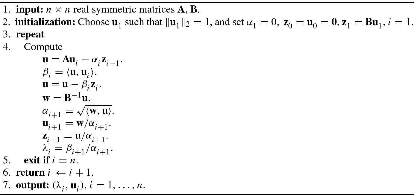
Algorithm 5.1 uses a contraction mapping to compute the generalized eigenpairs (λ, u) of a given n × n real symmetric matrix pencil (A, B).
Algorithm 5.2 is a tangent algorithm for computing the GEVD of a symmetric positive definite matrix pencil.

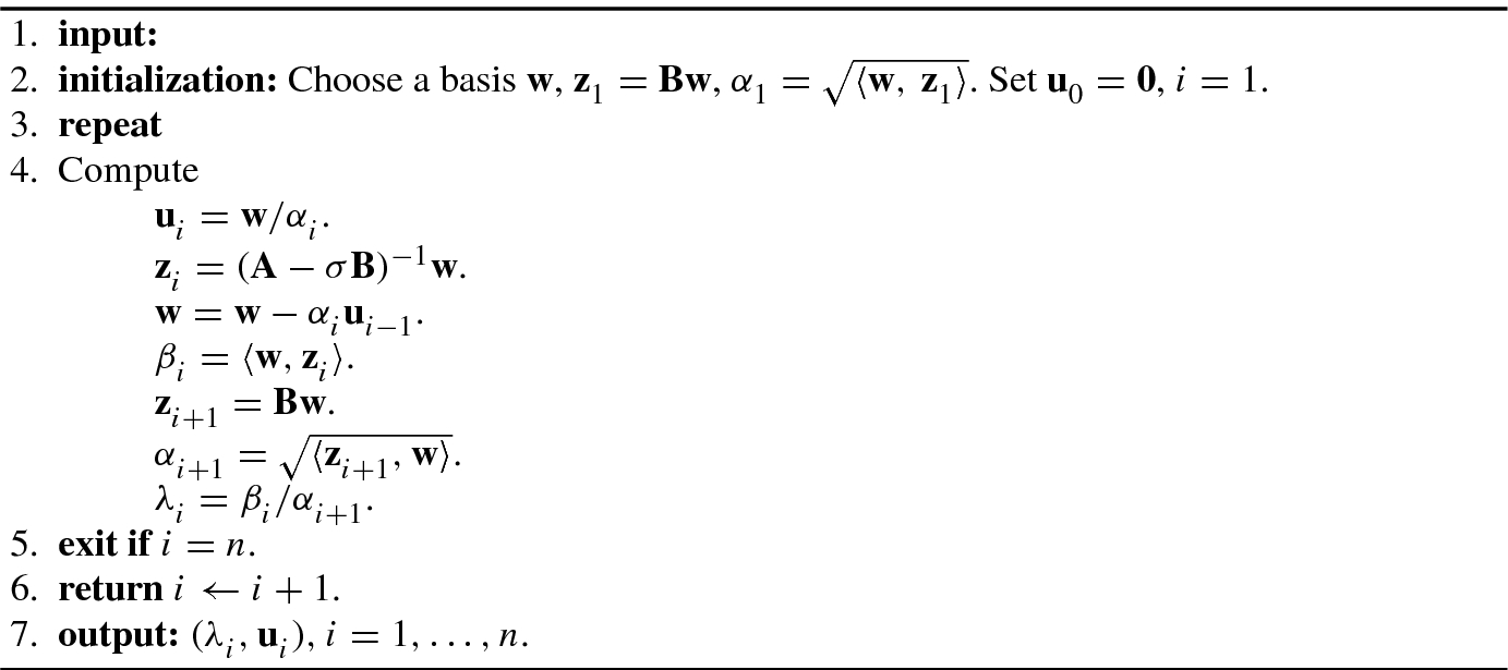
When the matrix B is singular, Algorithms 5.1 and 5.2 will be unstable. The GEVD algorithm for the matrix pencil (A, B) with singular matrix B was proposed by Nour-Omid et al. [12], this is shown in Algorithm 5.3. The main idea of this algorithm is to introduce a shift factor σ such that A − σB is nonsingular.
Two matrix pencils with the same generalized eigenvalues are known as equivalent matrix pencils.
 and the properties of a determinant it is easy to see that
If X and Y are two nonsingular matrices, then the matrix pencils (XAY, XBY) and (A, B) are equivalent.
The GEVD can be equivalently written as αAu = βBu as well. In this case, the generalized eigenvalue is defined as λ = β∕α.
5.3.2 Total Least Squares Method for GEVD
As shown by Roy and Kailath [16], use of a least squares estimator can lead to some potential numerical difficulties in solving the generalized eigenvalue problem. To overcome this difficulty, a higher-dimensional ill-conditioned LS problem needs to be transformed into a lower-dimensional well-conditioned LS problem.
Without changing its nonzero generalized eigenvalues, a higher-dimensional matrix pencil can be transformed into a lower-dimensional matrix pencil by using a truncated SVD.

 is composed of p principal singular values. Under the condition that the generalized eigenvalues remain unchanged, we can premultiply the matrix pencil A − γB by
  and postmultiply it by V
1 to get [18]:
and postmultiply it by V
1 to get [18]: 
 . The GEVD of the lower-dimensional matrix pencil
  is called the total least squares (TLS) method for the GEVD of the higher-dimensional matrix pencil (A, B), which was developed in [18].
5.4 Rayleigh Quotient and Generalized Rayleigh Quotient
In physics and artificial intelligence, one often meets the maximum or minimum of the quotient of the quadratic function of a Hermitian matrix. This quotient has two forms: the Rayleigh quotient (also called the Rayleigh–Ritz ratio) of a Hermitian matrix and the generalized Rayleigh quotient (or generalized Rayleigh–Ritz ratio) of two Hermitian matrices.
5.4.1 Rayleigh Quotient
In his study of the small oscillations of a vibrational system, in order to find the appropriate generalized coordinates, Rayleigh [15] in the 1930s proposed a special form of quotient, later called the Rayleigh quotient.
 is a scalar and is defined as

- 1.
Homogeneity: If α and β are scalars, then R(αx, βA) = βR(x, A).
- 2.
Shift invariance: R(x, A − αI) = R(x, A) − α.
- 3.
Orthogonality: x ⊥(A − R(x)I)x.
- 4.
Boundedness: When the vector x lies in the range of all nonzero vectors, the Rayleigh quotient R(x) falls in a complex plane region (called the range of A). This region is closed, bounded, and convex. If A is a Hermitian matrix such that A = A H, then this region is a closed interval
![$$[\lambda _1^{\,} ,\lambda _n^{\,} ]$$](../images/492994_1_En_5_Chapter/492994_1_En_5_Chapter_TeX_IEq69.png) .
. - 5.
Minimum residual: For all vectors x ≠ 0 and all scalars μ, we have ∥(A − R(x)I)x∥≤∥(A − μI)x∥.
 be a Hermitian matrix whose eigenvalues are arranged in increasing order:


More generally, the eigenvectors and eigenvalues of A correspond, respectively, to the critical points and the critical values of the Rayleigh quotient R(x).
This theorem has various proofs, see, e.g., [6, 7] or [3].

 has n Rayleigh quotients that are equal to n eigenvalues of A, namely R
i(x, A) = λ
i(A), i = 1, …, n.
has n Rayleigh quotients that are equal to n eigenvalues of A, namely R
i(x, A) = λ
i(A), i = 1, …, n.5.4.2 Generalized Rayleigh Quotient

 , where B
1∕2 denotes the square root of the positive definite matrix B. Substitute
, where B
1∕2 denotes the square root of the positive definite matrix B. Substitute  into the definition formula of the generalized Rayleigh quotient (5.4.6); then we have
 is selected as the eigenvector corresponding to the minimum eigenvalue
  of C, the generalized Rayleigh quotient takes a minimum value
  , while when the vector
  is selected as the eigenvector corresponding to the maximum eigenvalue
  of C, the generalized Rayleigh quotient takes the maximum value
  .
. . If
. If  is the EVD of the matrix B, then
Premultiplying  by B
−1∕2 and substituting (B
−1∕2)H = B
−1∕2, it follows that
by B
−1∕2 and substituting (B
−1∕2)H = B
−1∕2, it follows that  or B
−1Ax = λx. Hence, the EVD of the matrix product (B
−1∕2)HA(B
−1∕2) is equivalent to the EVD of B
−1A.
or B
−1Ax = λx. Hence, the EVD of the matrix product (B
−1∕2)HA(B
−1∕2) is equivalent to the EVD of B
−1A.


5.4.3 Effectiveness of Class Discrimination
Pattern recognition is widely applied in recognitions of human characteristics (such as a person’s face, fingerprint, iris) and various radar targets (such as aircraft, ships). In these applications, the extraction of signal features is crucial. For example, when a target is considered as a linear system, the target parameter is a feature of the target signal.
The divergence is a measure of the distance or dissimilarity between two signals and is often used in feature discrimination and evaluation of the effectiveness of class discrimination.
 denote the kth sample feature vector of the lth class of signals, where l = 1, …, c and k = 1, ⋯ , l
K, with l
K the number of sample feature vectors in the lth signal class. Under the assumption that the prior probabilities of the random vectors
denote the kth sample feature vector of the lth class of signals, where l = 1, …, c and k = 1, ⋯ , l
K, with l
K the number of sample feature vectors in the lth signal class. Under the assumption that the prior probabilities of the random vectors  are the same for k = 1, …, l
K (i.e., equal probabilities), the Fisher measure is defined as
are the same for k = 1, …, l
K (i.e., equal probabilities), the Fisher measure is defined as

 is the mean (centroid) of all signal-feature vectors of the lth class;
 is the variance of all signal-feature vectors of the lth class;
 is the total sample centroid of all classes.
As an extension of the Fisher measure, consider the projection of all Q × 1 feature vectors onto the (c − 1)th dimension of class discrimination space.
 , where
  represents the number of feature vectors of the ith class signal extracted in the training phase. Suppose that
 ![$${\mathbf {s}}_{i,k}^{\,} =[s_{i,k}^{\,} (1),\ldots ,s_{i,k}^{\,} (Q)]^T$$](../images/492994_1_En_5_Chapter/492994_1_En_5_Chapter_TeX_IEq91.png) denotes the Q × 1 feature vector obtained by the kth group of observation data of the ith signal in the training phase, while
denotes the Q × 1 feature vector obtained by the kth group of observation data of the ith signal in the training phase, while ![$${\mathbf {m}}_i^{\,} =[m_i^{\,} (1), \ldots ,m_i^{\,} (Q)]^T$$](../images/492994_1_En_5_Chapter/492994_1_En_5_Chapter_TeX_IEq92.png) is the sample mean of the ith signal-feature vector, where
is the sample mean of the ith signal-feature vector, where 


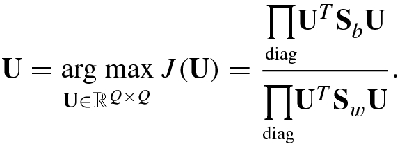
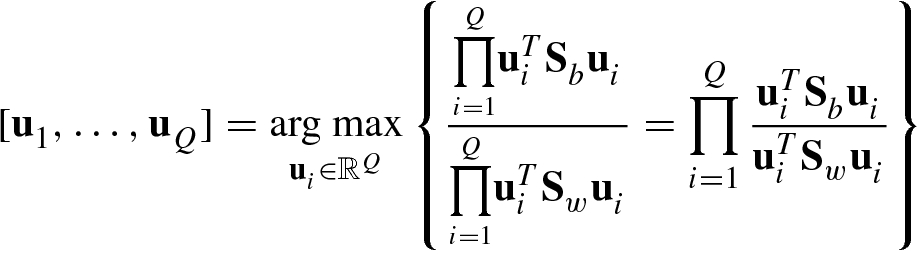
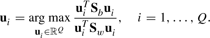

 . These generalized eigenvectors constitute the Q × (c − 1) matrix
 ![$$\displaystyle \begin{aligned} {\mathbf{U}}_{c-1}^{\,} =[{\mathbf{u}}_1^{\,} ,\ldots ,{\mathbf{u}}_{c-1}^{\,} ] \end{aligned} $$](../images/492994_1_En_5_Chapter/492994_1_En_5_Chapter_TeX_Equ41.png)
 , we can find its projection onto the optimal class discrimination subspace,
When there are only three classes of signals (c = 3), the optimal class discrimination subspace is a plane, and the projection of every feature vector onto the optimal class discrimination subspace is a point. These projections directly reflect the discrimination ability of different feature vectors in signal classification.
This chapter focuses on the matrix algebra used widely in artificial intelligence: eigenvalue decomposition, general eigenvalue decomposition, Rayleigh quotients, generalized Rayleigh quotients, and Fisher measure.