© Springer Nature Singapore Pte Ltd. 2020

X.-D. ZhangA Matrix Algebra Approach to Artificial Intelligencehttps://doi.org/10.1007/978-981-15-2770-8_9

9. Evolutionary Computation

Xian-Da Zhang¹  

(1)

Department of Automation, Tsinghua University, Beijing, Beijing, China

 

 Deceased

From the perspective of artificial intelligence, evolutionary computation belongs to computation intelligence. The origins of evolutionary computation can be traced back to the late 1950s (see, e.g., the influencing works [12, 15, 46, 47]), and has started to receive significant attention during the 1970s (see, e.g., [41, 68, 133]).

The first issue of the Evolutionary Computation in 1993 and the first issue of the IEEE Transactions on Evolutionary Computation in 1997 mark two important milestones in the history of the rapidly growing field of evolutionary computation.

This chapter is focused primarily on basic theory and methods of evolutionary computation, including multiobjective optimization, multiobjective simulated annealing, multiobjective genetic algorithms, multiobjective evolutionary algorithms, evolutionary programming, differential evolution together with ant colony optimization, artificial bee colony algorithms, and particle swarm optimization. In particular, this chapter also highlights selected topics and advances in evolutionary computation: Pareto optimization theory, noisy multiobjective optimization, and opposition-based evolutionary computation.

9.1 Evolutionary Computation Tree

Evolutionary computation can be broadly classified into three major categories.

1. 1.

   Physic-inspired evolutionary computation: Its typical representative is simulated annealing [100] inspired by heating and cooling of materials.

    
2. 2.

   Darwin’s evolution theory inspired evolutionary computation

   • Genetic Algorithm (GA) is inspired by the process of natural selections. A GA is commonly used to generate high-quality solutions to optimization and search problems by relying on bio-inspired operators such as mutation, crossover, and selection.

   • Evolutionary Algorithms (EAs) are inspired by Darwin’s evolution theory which is based on survival of fittest candidate for a given environment. These algorithms begin with a population (set of solutions) which tries to survive in an environment (defined with fitness evaluation). The parent population shares their properties of adaptation to the environment to the children with various mechanisms of evolution such as genetic crossover and mutation.

   • Evolutionary Strategy (ES) was developed by Schwefel in 1981 [143]. Similar to the GA, the ES uses evolutionary theory to optimize, that is to say, genetic information is used to inherit and mutate the survival of the fittest generation by generation, so as to get the optimal solution. The difference lies in: (a) the DNA sequence in ES is encoded by real number instead of 0-1 binary code in GA; (b) In the ES the mutation intensity is added for each real number value on the DNA sequence in order to make a mutation.

   • Evolutionary Programming (EP) [43]: The EP and the ES adopt the same coding (digital string) to the optimization problem and the same mutation operation mode, but they adopt the different mutation expressions and survival selections. Moreover, the crossover operator in ES is optional, while there is no crossover operator in EP. In the aspect of parent selection, the ES adopts the method of probability selection to form the parent, and each individual of the parent can be selected with the same probability, while the EP adopts a deterministic approach, that is, each parent in the current population must undergo mutation to generate offspring.

   • Differential Evolution (DE) was developed by Storn and Price in 1997 [147]. Similar to the GA, the main process includes three steps: mutation, crossover, and selection. The difference is that the GA controls the parent’s crossover according to the fitness value, while the mutation vector of the DE is generated by the difference vector of the parent generation, and crossover with the individual vector of the parent generation to generate a new individual vector, which directly selects with the individual of the parent generation. Therefore, the approximation effect of DE is more significant than that of the GA.

    
3. 3.
   Swarm intelligence inspired evolutionary computation: Swarm intelligence includes two important concepts: (a) The concept of a swarm means multiplicity, stochasticity, randomness, and messiness. (b) The concept of intelligence implies a kind of problem-solving ability through the interactions of simple information-processing units. This “collective intelligence” is built up through a population of homogeneous agents interacting with each other and with their environment. The major swarm intelligence inspired evolutionary computation includes:

   • Ant Colony Optimization (ACO) by Dorigo in 1992 [28]; a swarm of ants can solve very complex problems such as finding the shortest path between their nest and the food source. If finding the shortest path is looked upon as an optimization problem, then each path between the starting point (their nest) and the terminal (the food source) can be viewed as a feasible solution.

   • Artificial Bee Colony (ABC) algorithm, proposed by Karaboga in 2005 [81], is inspired by the intelligent foraging behavior of the honey bee swarm. In the ABC algorithm, the position of a food source represents a possible solution of the optimization problem and the nectar amount of a food source corresponds to the quality (fitness) of the associated solution.

   • Particle Swarm Optimization (PSO), developed by Kennedy and Eberhart in 1995 [86], is essentially an optimization technique based on swarm intelligence, and adopts a population-based stochastic algorithm for finding optimal regions of complex search spaces through the interaction of individuals in a population of particles. Different from evolutionary algorithms, the particle swarm does not use selection operation; while interactions of all population members result in iterative improvement of the quality of problem solutions from the beginning of a trial until the end.

    

The above classification of evolutionary computation can be represented by evolutionary computation tree, as shown in Fig. 9.1.

Fig. 9.1

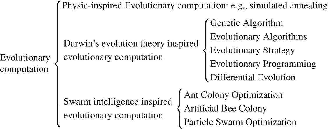
Evolutionary computation tree

9.2 Multiobjective Optimization

In science and engineering applications, a lot of optimization problems involve with multiple objectives. Different from single-objective problems, objectives in multiobjective problems are usually conflict. For example, in the design of a complex hardware/software system, an optimal design might be an architecture that minimizes cost and power consumption but maximizing the overall performance. This structural contradiction leads to multiobjective optimization theories and methods different from single-objective optimization. The need for solving multiobjective optimization problems has spawned various evolutionary computation methods.

This section discusses two multiobjective optimizations: multiobjective combinatorial optimization problems and multiobjective optimization problems.

9.2.1 Multiobjective Combinatorial Optimization

Combinatorial optimization is a topic that consists of finding an optimal object from a finite set of objects.

The general framework of multiobjective combinatorial optimization (MOCO) is described as [152]

(9.2.1)

(9.2.2)

where , the solution is a vector of discrete decision variables, and B = {0, 1}, and Ax ≤b denotes the elementwise inequality (Ax)_i ≤ b _i for all i = 1, …, m.

Most of multiobjective combinatorial optimization are related to assignment problems (APs), transportation problems (TPs) and network flow problems (NFPs).

1. 1.
   Multiobjective assignment problems [ 17]:

   

   (9.2.3)

   

   (9.2.4)

   

   (9.2.5)

   

   (9.2.6)
    
2. 2.
   Multiobjective transportation problems [ 152]:

   

   (9.2.7)

   

   (9.2.8)

   

   (9.2.9)

   

   (9.2.10)

   Here, it is not restrictive to suppose equality constraints with .

    
3. 3.
   Multiobjective network flow or transhipment problems [ 152]: Let G(N, A) be a network flow with a node set N and an arc set A; the model can be stated as

   

   (9.2.11)

   

   (9.2.12)

   

   (9.2.13)

   

   (9.2.14)

   where x _ij is the flow through arc (i, j), is the linear transhipment “cost” for arc (i, j) in objective k, and l _ij and u _ij are lower and upper bounds on x _ij, respectively.

    
4. 4.
   Multiobjective Min Sum Location Problems [ 134]:

   

   (9.2.15)

   

   (9.2.16)

   

   (9.2.17)

   

   (9.2.18)

   

   (9.2.19)

   where z _i = 1 if a facility is established at site i; x _ii = 1 if customer j is assigned to the facility at site i; d _ij is a certain usage of the facility at site i by customer j if he/she is assigned to that facility; a _i and b _i are possible limitations on the total customer usage permitted at the facility i; is, for objective k, a variable cost (or distance, etc.) if customer j is assigned to facility i; is, for objective k, a fixed cost associated with the facility at site i.

    

An unconstrained combinatorial optimization problem P = (S, f) is an optimization problem [120], where S is a finite set of solutions (called search space), and is an objective function that assigns a positive cost value to each solution vector s ∈ S. The goal is either to find a solution of minimum cost value or a good enough solution in a reasonable amount of time in the case of approximate solution techniques.

The difficulty of multiobjective combinatorial optimization problems comes from the following two factors [22].

• It requires intensive co-operation with the decision maker for solving a multiobjective combinatorial optimization problem; this results in especially high requirements for effective tools used to generate efficient solutions.

• Many combinatorial problems are hard even in single-objective versions; their multiple objective versions are frequently more difficult.

An multiobjective decision making (MODM) problem is ill-posed from the mathematical point of view because, except in trivial cases, it has no optimal solution. The goal of MODM methods is to find a solution most consistent with the decision maker’s preferences, i.e., the best compromise. Under very weak assumptions about decision maker’s preferences the best compromise solution belongs to the set of efficient solutions [136].

9.2.2 Multiobjective Optimization Problems

Consider optimization problems with multiple objectives that may usually be incompatible.

Definition 9.1 (Multiobjective Optimization Problem [78, 150])

A multiobjective optimization problem (MOP) consists of a set of n parameters (i.e., decision variables), a set of m objective functions, and a set of p inequality constraints and q equality constraints, and can be mathematically formulated as

(9.2.20)

(9.2.21)

(9.2.22)

Here the integer m ≥ 2 is the number of objectives; x = [x ₁, …, x _n]^T ∈ X is a decision vector, y = [y ₁, …, y _m]^T is the objective vector; are the objective functions, and are p inequality constraints and q equality constraints of the problem, respectively; while is called the decision space, and is known as the objective space.

The decision space and the objective space are two Euclidean spaces in MOPs:

• The n-dimensional decision space in which each coordinate axis corresponds to a component (called decision variable) of decision vector x.

• The m-dimensional objective space in which each coordinate axis corresponds to a component (i.e., a scalar objective function) of objective function vector y = f(x) = [f ₁(x), …, f _m(x)]^T.

The MOP’s evaluation function f : x →y maps decision vector x = [x ₁, …, x _n]^T to objective vector y = [y ₁, …, y _m]^T = [f ₁(x), …, f _m(x)]^T.

If some objective function f _i is to be maximized (or minimized), the original problem is written as the minimization (or maximization) of the negative objective − f _i. Thereafter, we consider only the multiobjective minimization (or maximization) problems, rather than optimization problems mixing both minimization and maximization.

The constraints g(x) ≤0 and h(x) = 0 determine the set of feasible solutions.

Definition 9.2 (Feasible Set)

The feasible set X _f is defined as the set of decision vectors x that satisfy the inequality constraint g(x) ≤0 and the equality constraint h(x) = 0, i.e.,

(9.2.23)

Example 9.1

Dynamic economic emission dispatch problem is a typical multiobjective optimization which attempts to minimize both cost function and emission function simultaneously while satisfying equality and inequality constraints [8].

1. 1.
   Objectives:

   • Cost function: The fuel cost function of each thermal generator, considering the valve-point effect, is expressed as the sum of a quadratic and a sinusoidal function. The total fuel cost in terms of real power can be expressed as

     

     (9.2.24)

     where N is number of generating units, M is number of hours in the time horizon; a _i, b _i, c _i, d _i, e _i are cost coefficients of the ith unit; P _im is power output of ith unit at time m, and is lower generation limits for ith unit.

   • Emission function: The atmospheric pollutants such as sulfur oxides (SOx) and nitrogen oxides (NOx) caused by fossil-fueled generating units can be modeled separately. However, for comparison purpose, the total emission of these pollutants which is the sum of a quadratic and an exponential function can be expressed as

     

     (9.2.25)

     where α _i, β _i, γ _i, η _i, δ _i are emission coefficients of the ith unit.

    
2. 2.
   Constraints:

   • Real power balance constraints: The total real power generation must balance the predicted power demand plus the real power losses in the transmission lines, at each time interval over the scheduling horizon, i.e.,

     

     (9.2.26)

     where P _Dm is load demand at time m, P _Lm is transmission line losses at time m.

   • Real power operating limits:

     

     (9.2.27)

     where is upper generation limits for the ith unit.

   • Generating unit ramp rate limits:

     

     (9.2.28)
     

     (9.2.29)

     where UR _i and DR _i are ramp-up and ramp-down rate limits of the ith unit, respectively.

    

Definition 9.3 (Ideal Vector [20, p. 8])

Let be a vector of variables which optimizes (either minimizes or maximizes) the kth objective function f _k(x). In other words, if the vector x ^{opt, k} ∈ X _f is such that

(9.2.30)

then the objective vector (where denotes the optimum of the kth objective function) is ideal for an MOP, and the point in which determined this vector is the ideal solution, and is consequently called the ideal vector.

However, due to objective conflict and/or interdependence among the n decision variables of x, such an ideal solution vector is impossible for MOPs: none of the feasible solutions allows simultaneous optimal solutions for all objectives [63].

In other words, individual optimal solutions for each objective are usually different. Thus, a mathematically most favorable solution should offer the least objective conflict.

Many real-life problems can be described as multiobjective optimization problems. The most typical multiobjective optimization problem is traveling salesman problem.

The traveling salesman problem (TSP) can be stated as (see, e.g., [152])

(9.2.31)

where ρ(i) is a tour of {1, …, n} and k denotes trip k.

Let be a set of cities, where c _i is the ith city and N _c is the number of all cities; A = {(r, s) : r, s ∈ C} be the edge set, and d(r, s) be a cost measure associated with edge (r, s) ∈ A.

For a set of N _c cities, the TSP problem involves finding the shortest length closed tour visiting each city only once. In other words, the TSP problem is to find the shortest-route to visit each city once, ending up back at the starting city.

The following are the different forms of TSP [105]:

• Euclidean TSP: If cities r ∈ C are given by their coordinates (x _r, y _r) and d(r, s) is the Euclidean distance between city r and s, then TSP is an Euclidean TSP.

• Symmetric TSP: If d(r, s) = d(s, r) for all (r, s), then the TSP becomes a symmetric TSP (STSP).

• Asymmetric TSP: If d(r, s) ≠ d(s, r) for at least some (r, s), then the TSP is an asymmetric TSP (ATSP).

• Dynamic TSP: The dynamic TSP (DTSP) is a TSP in which cities can be added or removed at run time.

The goal of TSP is to find the shortest closed tour which visits all the cities in a given set as early as possible after each and every iteration.

Another typical example of multiobjective optimizations is multiobjective data mining.

One of the most important questions in data mining problems is how to evaluate a candidate model which depends on the type of data mining task at hand. Data mining involves discovering interesting and potentially useful patterns of different types, such as associations, summaries, rules, changes, outliers, and significant structures [110]. Data mining tasks can broadly be classified into two categories [6, 62]:

• Predictive or supervised techniques learn from the current data in order to make predictions about the behavior of new data sets.

• Descriptive or unsupervised techniques provide a summary of the data.

The most commonly used data mining tasks include feature selection, classification, regression, clustering, association rule mining, deviation detection, and so on [110].

1. 1.
   Feature Selection: It deals with selection of an optimum relevant set of features or attributes that are necessary for the recognition process (classification or clustering). In general, the feature selection problem ( Ω, P) can formally be defined as an optimization problem: determine the feature set F ^∗ for which

   

   (9.2.32)

   where Ω is the set of possible feature subsets, F refers to a feature subset, and denotes a criterion to measure the quality of a feature subset with respect to its utility in classifying/clustering the set of points X ∈ Ψ.

    
2. 2.

   Classification: The problem of supervised classification can formally be stated as follows. Given an unknown function g : X → Y  (the ground truth) that maps input instances x ∈ X to output class labels y ∈ Y , and a training data set D = {(x ₁, y ₁), …, (x _n, y _n)} which is assumed to represent accurate examples of the mapping g, produce a function h : X → Y  that approximates the correct mapping g as closely as possible.

    
3. 3.
   Clustering: Clustering is an important unsupervised classification technique where a set of n patterns are grouped into clusters {C ₁, …, C _K} in such a way that patterns in the same cluster are similar in some sense and patterns in different clusters are dissimilar in the same sense. The main objective of any clustering technique is to produce a K × n partition matrix U = [u _kj], k = 1, …, K;j = 1, …, n, where u _kj is the membership of pattern x _j to cluster C _k:

   

   (9.2.33)

   for hard or crisp partitioning of the data, and

   

   (9.2.34)

   

   (9.2.35)

   with for probabilistic fuzzy partitioning of the data.

    
4. 4.

   Association Rule Mining: The principle of association rule mining (ARM) [1] lies in the market basket or transaction data analysis. Association analysis is the discovery of rules showing attribute-value associations that occur frequently. The objective of ARM is to find all rules of the form X ⇒ Y, X ∩ Y = ∅ with probability c%, indicating that if itemset X occurs in a transaction, the itemset Y  also occurs with probability c%.

    

Most of the data mining problems can be thought of as optimization problems, while the majority of data mining problems have multiple criteria to be optimized. For example, a feature selection problem may try to maximize the classification accuracy while minimizing the size of the feature subset. Similarly, a rule mining problem may optimize several rule interestingness measures such as support, confidence, comprehensibility, and lift at the same time [110, 148].

9.3 Pareto Optimization Theory

Many real-world problems in artificial intelligence involve simultaneous optimization of several incommensurable and often competing objectives. In these cases, there may exist solutions in which the performance on one objective cannot be improved without reducing performance on at least one other. In other words, there is often no single optimal solution with respect to all objectives. In practice, there could be a number of optimal solutions in multiobjective optimization problems (MOPs) and the suitability of one solution depends on a number of factors including designer’s choice and problem environment. These solutions are optimal in the wider sense that no other solutions in the search space are superior to them when all objectives are considered. In these problems, the Pareto optimization approach is a natural choice. Solutions given by the Pareto optimization approach are called Pareto-optimal solutions that are closely related to Pareto concepts.

9.3.1 Pareto Concepts

Pareto concepts are named after Vilfredo Pareto (1848–1923). These concepts constitute the Pareto optimization theory for multiple objectives.

Consider the multiobjective optimization problems

(9.3.1)

in which the objectives (or criterion functions) f _l, …, f _m are real-valued, continuous, and quasi-concave (for maximization) or quasi-convex (for minimization) on a closed convex set S.

Three approaches can be taken to find the solution(s) to the above problems [10].

• Reformulation approach: This approach entails reformulating the problem as a single objective problem. To do so, additional information is required from the decision makers, such as the relative importance or weights of the objectives, goal levels for the objectives, value functions, etc.

• Decision making approach: This approach requires that the decision makers interact with the optimization procedure typically by specifying preferences between pairs of presented solutions.

• Pareto optimization approach: It finds a representative set of nondominated solutions approximating the Pareto front. Pareto optimization methods, such as evolutionary multiobjective optimization algorithms, allow decision makers to investigate the potential solutions without a priori judgments regarding to the relative importance of objective functions. Post-Pareto analysis is necessary to select a single solution for implementation.

On the other hand, the most distinguishing feature of single objective evolutionary algorithms (EAs) compared to other heuristics is that EAs work with a population of solutions, and thus are able to search for a set of solutions in a single run. Due to this feature, single objective evolutionary algorithms are easily extended to multiobjective optimization problems. Multiobjective evolutionary algorithms (MOEAs) have become one of the most active research areas in evolutionary computation.

To describe the Pareto optimality of MOP solutions in which we are interested, it needs the following key Pareto concepts: Pareto dominance, Pareto optimality, the Pareto-optimal set, and the Pareto front.

For the convenience of narration, denote x = [x ₁, …, x _n]^T ∈ F ⊆ S and , where F is the feasible region, in which the constraints are satisfied.

Definition 9.4 (Vector Function Relation [150])

For any two objective vectors f(x) and f(x′), their relations are written as

(9.3.2)

(9.3.3)

and

(9.3.4)

(9.3.5)

(9.3.6)

(9.3.7)

Here the symbol ∧ may be interpreted as logical conjunction operator (“AND”).

It goes without saying that the above relations are available for f(x) = x and f(x′) = x′ as well. However, for two decision vectors x and x′, these relations are meaningless. In multiobjective optimization, the relation between decision vectors x and x′ are called the Pareto dominance which is based on the relations between vector objective functions.

Definition 9.5 (Pareto Dominance [150, 171])

For any two decision vectors x and x′ in minimization problems, x is said to dominate (or outperform) x′, denoted by x ≻x′, if and only if their objectives or outcomes satisfy jointly the following two conditions:

1. 1.

   x is no worse than x′ in all objective functions, i.e., f _i(x) ≤ f _i(x′) for all i ∈{1, …, m},

    
2. 2.

   x is strictly better than x′ for at least one objective function, i.e., f _j(x) < f _j(x′) for at least one j ∈{1, …, m};

    

oris equivalently represented as

(9.3.8)

or simply written as

(9.3.9)

Similarly, for maximization problems, then

(9.3.10)

or simply written as

(9.3.11)

The Pareto dominance can be either weak or strong.

Definition 9.6 (Weak Pareto Dominance [150, 171])

A decision vector x is said to weakly dominate another decision vector x′, denoted by x ≽x′, if and only if

(9.3.12)

(9.3.13)

Definition 9.7 (Strict Pareto Dominance [171])

A decision vector x is said to strictly dominate x′, denoted by x ≻≻x′, if and only if f _i(x) is better than f _i(x′) in all objectives, i.e.,

(9.3.14)

(9.3.15)

Definition 9.8 (Incomparable [150, 171])

Two decision vectors x and x′ are said to be incomparable, denoted by x ∥x′, if neither x weakly dominates x′ nor x′ weakly dominates x, i.e.,

(9.3.16)

Two incomparable solutions x and x′ are also known as mutually nondominating.

Definition 9.9 (Nondominance [144, 171])

A decision vector x ∈ X _f is said to be nondominated regarding a set A ⊆ X _f if and only if there is no vector a in A which dominates x; formally

(9.3.17)

In other words, a solution x is said to be a nondominated solution if there is no a in the subset A that dominates x.

A Pareto improvement is a change to a different allocation that makes at least one objective better off without making any other objective worse off. An trial solution is known as “Pareto efficient” or “Pareto-optimal” or “globally nondominated” when no further Pareto improvements can be made, in which case we are assumed to have reached Pareto optimality.

Definition 9.10 (Pareto-Optimality [144, 171])

A decision vector x ∈ X _f is said to be Pareto-optimal if and only if x is nondominated regarding the feature region X _f, namely

(9.3.18)

In other words, all decision vectors which are not dominated by any other decision vector are known as “nondominated” or Pareto optimal. The phrase “Pareto optimal” means the solution is optimal with respect to the entire decision variable space F unless otherwise specified.

Figure 9.2, by inferencing Economics Wiki on “Pareto Efficient and Pareto Optimal Tutorial,” shows the relation of the Pareto efficiency and Pareto improvement for the two-objective minimization problems min_xf(x) = [f ₁(x), f ₂(x)]^T.

Fig. 9.2

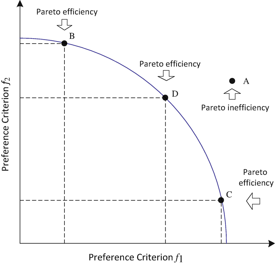
Pareto efficiency and Pareto improvement. Point A is an inefficient allocation between preference criterions f ₁ and f ₂ because it does not satisfy the constraint curve of f ₁ and f ₂. Two decisions to move from Point A to Points C and D would be a Pareto improvement, respectively. They improve both f ₁ and f ₂, without making anyone else worse off. Hence, these two moves would be a Pareto improvement and be Pareto optimal, respectively. A move from Point A to Point B would not be a Pareto improvement because it decreases the cost f ₁ by increasing another cost f ₂, thus making one side better off by making another worse off. The move from any point that lies under the curve to any point on the curve cannot be a Pareto improvement due to making one of two criterions f ₁ and f ₂ worse

A nondominated decision vector in A ⊆ X _f is only Pareto-optimal in a local decision space A, while a Pareto-optimal decision vector is Pareto-optimal in entire feature decision space X _f. Therefore, a Pareto-optimal decision vector is definitely nondominated, but a nondominated decision vector is not necessarily Pareto-optimal.

However, to find Pareto-optimal solutions still is not the ultimate aim of multi-objective optimization, this is because:

• There may be a large number of Pareto-optimal solutions. To gain the deeper insight into the multiobjective optimization problem and knowledge about alternate solutions, there is often a special interest in finding or approximating the Pareto-optimal set.

• Due to conflicting objectives it is only possible to obtain a set of trade-off solutions (referred to as Pareto-optimal set in decision space or Pareto-optimal front in objective space), instead of a single optimal solution.

Therefore our aim is to find the decision vectors that are nondominated within the entire search space. These decision vectors constitute the so-called Pareto-optimal set, as defined below.

Definition 9.11 (Nondominated Sets [150])

Let A ⊆ X _f and the function g(A) give the set of nondominated decision vectors in A:

(9.3.19)

The set g(A) is said to be the nondominated set (NS) with respect to A. When A = X _f, the corresponding set

(9.3.20)

(9.3.21)

is known as the nondominated set in the entire decision space for minimization and maximization, respectively.

Definition 9.12 (Pareto-Optimal Set [150])

The Pareto-optimal set (PS) is the set of all objectives given by nondominated decision vectors x in nondominated set NS, namely

(9.3.22)

(9.3.23)

Here and are the Pareto-optimal sets for minimization and maximization, respectively.

Pareto-optimal decision vectors cannot be improved in any objective without causing a degradation in at least one other objective; they represent globally optimal solutions. Analogous to single-objective optimization problems, Pareto-optimal sets are divided into local and global Pareto-optimal sets.

Definition 9.13 (Local Pareto-Optimal Set [23, 171])

Consider a set of decision vectors X′⊆ X _f. The set X′ is said to be a local Pareto-optimal set if and only if

(9.3.24)

where ∥⋅∥ is a corresponding distance metric and 𝜖 > 0, δ > 0.

Definition 9.14 (Global Pareto-Optimal Set [23, 171])

The set X′ is called a global Pareto-optimal set if and only if

(9.3.25)

The set of all objectives given by Pareto-optimal set of decision vectors is known as the Pareto-optimal front (or simply called Pareto front).

Definition 9.15 (Pareto Front)

Given an objective vector f(x)                                      =                                      [f ₁(x), …, f _m(x)]^T and a Pareto-optimal set PS, the Pareto front PF is defined as the set of all objective vectors given by decision vectors x ∈ PS, i.e.,

(9.3.26)

Solutions in the Pareto front represent the possible optimal trade-offs between competing objectives.

For a given system, the Pareto frontier is the set of parameterizations (allocations) that are all Pareto efficient or Pareto optimal. Finding Pareto frontiers is particularly useful in engineering. This is because that when yielding all of the potentially optimal solutions, a designer needs only to focus on trade-offs within this constrained set of parameters without considering the full range of parameters.

It should be noted that a global Pareto-optimal set does not necessarily contain all Pareto-optimal solutions.

Pareto-optimal solutions are those solutions within the genotype search space (i.e., decision space) whose corresponding phenotype objective vector components cannot be all simultaneously improved. These solutions are also called non-inferior, admissible, or efficient solutions [73] in the sense that they are nondominated with respect to all other comparison solution vector and may have no clearly apparent relationship besides their membership in the Pareto-optimal set.

A “current” set of Pareto-optimal solutions is denoted by P _current(t), where t represents the generation number. A secondary population storing nondominated solutions found through the generations is denoted by P _known, while the “true” Pareto-optimal set, denoted by P _true, is not explicitly known for MOP problems of any difficulty. The associated Pareto front for each of P _current(t), P _known, and P _true are termed as PF _current(t), PF _known, and PF _true, respectively.

The decision maker is often selecting solutions via choice of acceptable objective performance, represented by the (known) Pareto front. Choosing an MOP solution that optimizes only one objective may well ignore “better” solutions for other objectives.

We wish to determine the Pareto-optimal set from the set X of all the decision variable vectors that satisfy the inequality constraints (9.2.21) and (9.2.22). But, not all solutions in the Pareto-optimal set are normally desirable or achievable in practice. For example, we may not wish to have different solutions that map to the same values in objective function space.

Lower and upper bounds on objective values of all Pareto-optimal solutions are given by the ideal objective vector f ^ideal and the nadir objective vectors f ^nad, respectively. In other words, the Pareto front of a multiobjective optimization problem is bounded by a nadir objective vector z ^nad and an ideal objective vector z ^ideal, if these are finite.

Definition 9.16 (Nadir Objective Vector, Ideal Objective Vector)

The nadir objective vector is defined as

(9.3.27)

and the ideal objective vector as

(9.3.28)

In other words, the components of a nadir and an ideal objective vector define upper and lower bounds for the objective function values of Pareto-optimal solutions, respectively. In practice, the nadir objective vector can only be approximated as, typically, the whole Pareto-optimal set is unknown. In addition, because of numerical reasons a utopian objective vector z ^utopian with elements

(9.3.29)

or in vector form

(9.3.30)

is often defined, where 𝜖 > 0 is a small constant, and 1 is an K-dimensional vector of all ones.

Definition 9.17 (Archive)

Nondominated set produced by heuristic algorithms is referred to as the archive (denoted by A) of the estimated Pareto front.

The archive of estimated Pareto fronts will only be an approximation to the true Pareto front.

When solving multiobjective optimization problems, since there are many possible Pareto-optimal solutions rather than a single optimal solution for possibly contradictory multiobjective functions, we need to organize or partition found solutions for selecting appropriate solution(s). The selection methods for Pareto-optimal solutions are divided to the following four categories:

• Fitness selection approach,

• Nondominated sorting approach,

• Crowding distance assignment approach, and

• Hierarchical clustering approach.

9.3.2 Fitness Selection Approach

To fairly evaluate the quality of each solution and make the solution set search in the direction of Pareto-optimal solution, how to implement fitness assignment is important.

There are benchmark metrics or indicators that play an important role in evaluating the Pareto fronts. These metrics or indicators are: hypervolume, spacing, maximum spread, and coverage [139].

Definition 9.18 (Hypervolume [170])

For a nondominated vector , its hypervolume (HV) is defined as

(9.3.31)

where is the area in the objective search space covered by the obtained Pareto front, and a _i is the hypervolume determined by the components of x ⁱ and the origin.

Definition 9.19 (Spacing)

Spacing is a measure for the spread (distribution) of nondominated solutions throughout the Pareto front. Actually, it measures the variance of the distance between adjacent nondominated solutions and can be evaluated by Santana et al. [139]

(9.3.32)

where is the mean distance between all the adjacent solutions and m is the number of nondominated solutions in the Pareto front, and

(9.3.33)

A value of spacing equal to zero means that all the solutions are equidistantly spaced in the Pareto front.

Definition 9.20 (Maximum Spread)

This metric, proposed by Zitzler et al. [171], evaluates the maximum extension covered by the nondominated solutions in the Pareto front, and can be calculated by

(9.3.34)

where m is the number of solutions in the Pareto front and K is the number of objectives in a given problem. It should be noted that higher values MS indicate better performance.

Definition 9.21 (Coverage)

The coverage metric of two sets A and B, proposed by Zitzler and Thiele [170], is denoted by C(A, B), and maps the ordered pair (A, B) to the interval [0, 1] using

(9.3.35)

where |B| is the number of elements of the set B.

The value C(A, B) = 1 means that all solutions in B are weakly dominated by ones in A. On the other hand, C(A, B) = 0 means that none of the solutions in B is weakly dominated by A. It should be noted that both C(A, B) and C(B, A) have to be evaluated, respectively, since C(A, B) is not necessarily equal to 1 − C(B, A).

If 0 < C(A, B) < 1 and 0 < C(B, A) < 1, then neither A weakly dominates B nor B weakly dominates A. Thus, the sets A and B are incomparable, which means that A is not worse than B and vice versa.

Two popular fitness selections are the binary tournament selection and the roulette wheel selection [140].

1. 1.

   Binary tournament selection: k individuals are drawn from the entire population, allowing them to compete (tournament) and extract the best individual among them. The number k is the tournament size, and often takes 2. In this special case, we can call it binary tournament selection. Tournament selection is just the broader term where k can be any number ≥ 2.

    
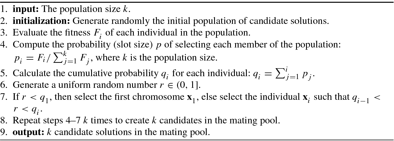
2. 2.
   Roulette wheel selection: It is also known as fitness proportionate selection which is a genetic operator for selecting potentially useful solutions for recombination. In roulette wheel selection, as in all selection methods, the fitness function assigns a fitness to possible solutions or chromosomes. This fitness level is used to associate a probability of selection with each individual chromosome. If F _i is the fitness of individual i in the population, its probability of being selected is

   

   (9.3.36)

   where N is the number of individuals in the population.

    

Algorithm 9.1 gives a roulette wheel fitness selection algorithm.

Algorithm 9.1 Roulette wheel fitness selection algorithm [140]

9.3.3 Nondominated Sorting Approach

The nondominated selection is based on nondominated rank: dominated individuals are penalized by subtracting a small fixed penalty term from their expected number of copies during selection. But this algorithm failed when the population had very few nondominated individuals, which may result in a large fitness value for those few nondominated points, eventually leading to a high selection pressure.

The idea behind the nondominated sorting procedure is twofold.

• Use a ranking selection method to emphasize good points.

• Use a niche method to maintain stable subpopulations of good points.

If an individual (or solution) is not dominated by all other individuals, then it is assigned as the first nondominated level (or rank). An individual is said to have the second nondominated level or rank, if it is dominated only by the individual(s) in the first nondominated level. Similarly, one can define individuals in the third or higher nondominated level or rank. It is noted that more individuals maybe have the same nondominated level or rank. Let i _rank represent the nondominated rank of the ith individual. For two solutions with different nondomination ranks, if i _rank < j _rank then the ith solution with the lower (better) rank is preferred.

Algorithm 9.2 shows a fast nondominated sorting approach.

Algorithm 9.2 Fast-nondominated-sort(P) [25]

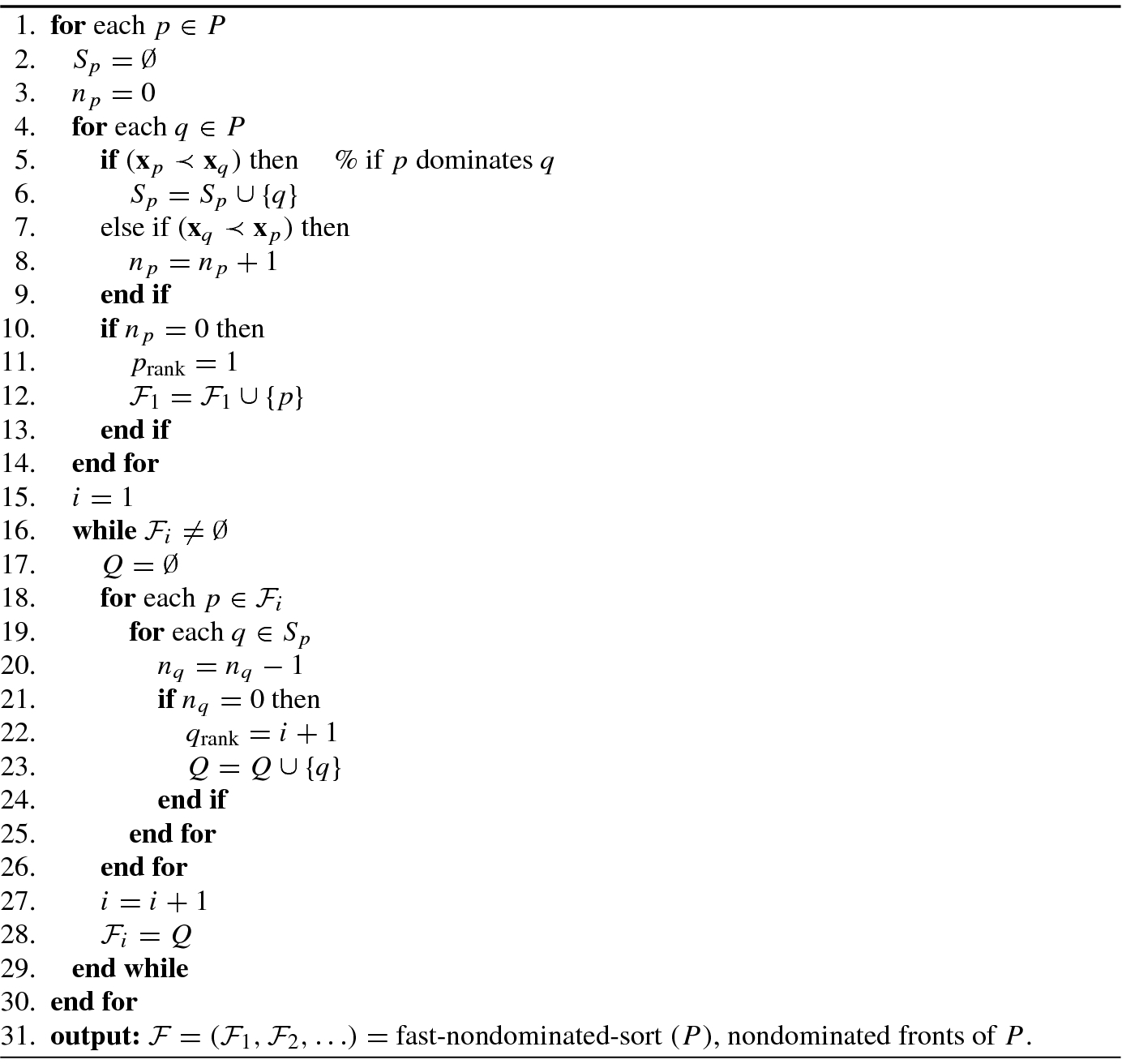
In order to identify solutions of the first nondominated front in a population of size N _P, each solution can be compared with every other solution in the population to find if it is dominated. At this stage, all individuals in the first nondominated level in the population are found. In order to find the individuals in the second nondominated level, the solutions of the first level are discounted temporarily and the above procedure is repeated for finding third and higher levels or ranks of nondomination.

9.3.4 Crowding Distance Assignment Approach

If the two solutions have the same nondominated rank (say i _rank = j _rank), which one should we choose? In this case, we need another quality for selecting the better solution. A natural choice is to estimate the density of solutions surrounding a particular solution in the population. For this end, the average distance of two points on either side of this point along each of the objectives needs to be calculated.

Definition 9.22 (Crowding Distance [132])

Let f ₁ and f ₂ be two objective functions in a multiobjective optimization problem, and let x, x _i and x _j be the members of a nondominated list of solutions. Furthermore, x _i and x _j are the nearest neighbors of x in the objective spaces. The crowding distance (CD) of a trial solution x in a nondominated set depicts the perimeter of a hypercube formed by its nearest neighbors (i.e., x _i and x _j) at the vertices in the fitness landscapes.

The crowding distance computation requires sorting the population according to each objective function value in ascending order of magnitude. Let the population consist of |I| individuals which are ranked according to their fitness values from small to large, and let denote the kth objective function of the ith individual, where i = 1, …, |I| and k = 1, …, K. Except for boundary individuals 1 and |I|, the ith individual in all other intermediate population set {2, …, |I|− 1} is assigned a finite crowded distance (CD) value given by Luo et al. [98]:

(9.3.37)

or [25, 163]

(9.3.38)

while the distance values of boundary individuals are assigned as CD ₁ = CD _|I| = ∞. Here, and are the maximum and minimum values of the kth objective of all individuals, respectively.

The crowded-comparison operator guides the selection process at the various stages of the algorithm toward a uniformly spread-out Pareto-optimal front. Every population has two attributes: nondomination rank and crowding distance. By combining the nondominated rank and the crowded distance, the crowded-comparison operator is defined by partial order (≺_n) as [25]:

(9.3.39)

That is, between two solutions with differing nondomination ranks, the solution with the lower (better) rank is preferred. Otherwise, if both solutions belong to the same front, then the solution that is located in a lesser crowded region is preferred. Therefore, the crowded-comparison operator (≺_n) guides the selection process at the various stages of the algorithm toward a uniformly spread-out Pareto-optimal front.

Algorithm 9.3 shows the crowding-distance-assignment (I).

Algorithm 9.3 Crowding-distance-assignment (I) [25]

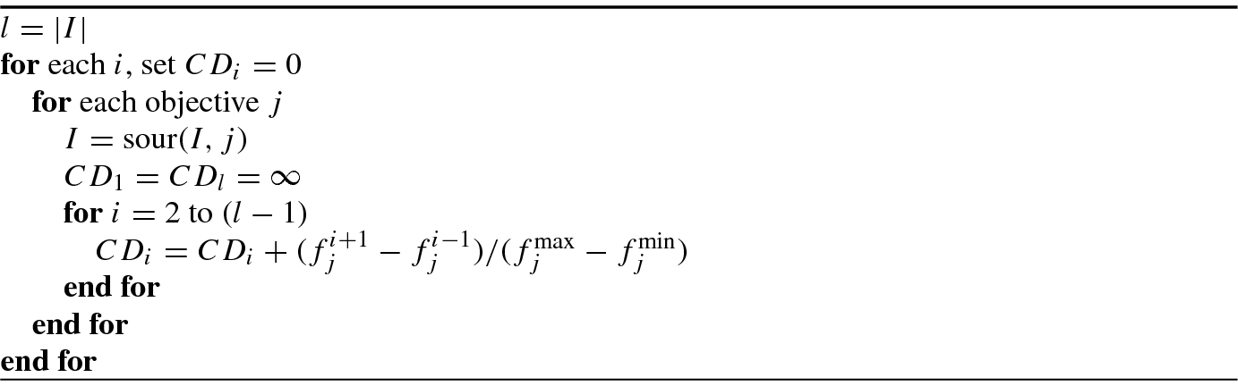
Between two populations with differing nondomination ranks, the population with the lower (better) rank is preferred. If both populations belong to the same front, then the population with larger crowding distance is preferred.

9.3.5 Hierarchical Clustering Approach

Cluster analysis can be applied to the results of a multiobjective optimization algorithm to organize or partition solutions based on their objective function values.

The steps of hierarchical clustering methodology are given below [108]:

1. 1.

   Define decision variables, feasible set, and objective functions.

    
2. 2.

   Choose and apply a Pareto optimization algorithm.

    
3. 3.
   Clustering analysis:

   • Clustering tendency: By visual inspection or data projections verify that a hierarchical cluster structure is a reasonable model for the data.

   • Data scaling: Remove implicit variable weightings due to relative scales using range scaling.

   • Proximity: Select and apply an appropriate similarity measure for the data, here, Euclidean distance.

   • Choice of algorithm(s): Consider the assumptions and characteristics of clustering algorithms and select the most suitable algorithm for the application, here, group average linkage.

   • Application of algorithm: Apply the selected algorithm to obtain a dendrogram.

   • Validation: Examine the results based on application subject matter knowledge, assess the fit to the input data and stability of the cluster structure, and compare the results of multiple algorithms, if used.

    
4. 4.

   Represent and use the clusters and structure: If the clustering is reasonable and valid, examine the divisions in the hierarchy for trade-offs and other information to aid decision making.

    

9.3.6 Benchmark Functions for Multiobjective Optimization

When designing an artificial intelligence algorithm or system, we need select the benchmark or test functions to examine its effectiveness in converging and maintaining a diverse set of nondominated solutions. A very simple multiobjective test function is the well-known one-variable two-objective function used by Schaffer [141]. It is defined as follows:

(9.3.40)

where x ∈ [0, 2].

The following are the several commonly used multiobjective benchmark functions.

1. 1.
   Benchmark functions for

   • ZDT1 functions [171]

     

     (9.3.41)

     where m = 30, x _i ∈ [0, 1].

   • ZDT4 functions [171]

     

     (9.3.42)

     where m = 10 and x _i ∈ [0, 1].

   • ZDT6 functions [171]:

     

     (9.3.43)

     where m = 10 and x _i ∈ [0, 1].

    
2. 2.
   Benchmark functions for

   • QV functions [126]

     

     (9.3.44)

     where x _i ∈ [−5, 5].

   • KUR functions [90]

     

     (9.3.45)

     where x _i ∈ [−10³, 10³].

    
3. 3.
   Constrained benchmark functions

   • Partially separable benchmark functions [23, 171]

     

     (9.3.46)
     where x = [x ₁, …, x _n]^T, the function f ₁ is a function of the first decision variable x ₁ only, g is a function of the remaining n − 1 variables x ₂, …, x _n, and the parameters of h are the function values of f ₁ and g. For example,

     

     (9.3.47)

     where n = 30 and x _i ∈ [0, 1]. The Pareto-optimal front is formed with g(x) = 1.

   • Separable benchmark functions [170]:

     

     (9.3.48)

     In this test, x is a 500-dimensional binary vector, a _ij is the profit of item j according to knapsack i, b _ij is the weight of item j according to knapsack i, and c _i is the capacity of knapsack i (i = 1, 2 and j = 1, 2, …, 500).

    
4. 4.
   Multiobjective benchmark functions for : SPH-m functions [92, 141]

   

   (9.3.49)

   where x _i ∈ [−10³, 10³].

    
5. 5.
   Multiobjective benchmark functions for

   • ISH1 functions [79]

     

     (9.3.50)

     where the value of α ∈ [0, 1] can be viewed as the correlation strength. α = 0 corresponds to the minimum correlation strength 0, where g _i(x) is the same as the randomly generated objective f _i(x). α = 1 corresponds to the maximum correlation strength 1, where g _i(x) is the same as f ₁(x) or f ₂(x).

   • ISH2 functions [79]

     

     (9.3.51)
     where α _ik is specified as follows:

     

     (9.3.52)
     For example, the four-objective problem is specified as

     

     (9.3.53)
    

More benchmark test functions can be found in [149, 165, 172]. Yao et al. [165] summarized 23 benchmark test functions.

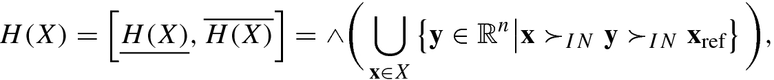
9.4 Noisy Multiobjective Optimization

Optimization problems in various real-world applications are often characterized by multiple conflicting objectives and a wide range of uncertainty. Optimization problems containing uncertainty and multiobjectives are termed as uncertain multiobjective optimization problems. In evolutionary optimization community, uncertainty in the objective functions is generally stochastic noise, and the corresponding multiobjective optimization problems are termed as noisy (or imprecise) multiobjective optimization problems.

Noisy multiobjective optimization problems are also known as interval multiobjective optimization problems, since objectives f _i(x, c _i) contaminated by noise vector c _i can be reformulated, in interval-value form, as .

9.4.1 Pareto Concepts for Noisy Multiobjective Optimization

There are at least two different types of uncertainty that are important for real-world modeling [96].

1. 1.

   Noise, also referred to as aleatory uncertainty. Noise is an inherent property of the system modeled (or is introduced into the model to simulate this behavior) and therefore cannot be reduced. By Oberkampf et al. [117], aleatory uncertainty is defined as the “inherent variation associated with the physical system or the environment under consideration.”

    
2. 2.

   Imprecision, also known as epistemic uncertainty, describes not uncertainty due to system variance but the uncertainty of the outcome due to “any lack of knowledge or information in any phase or activity of the modeling process” [117].

    

Uncertainty in objectives can be divided into two kinds [58].

• Decision vector corresponding to different objectives is no longer a fixed point, but is characterized by (x, c) with c = [c ₁, …, c _d]^T that is a local neighborhood of x, where is an interval with lower limits and upper limit for i = 1, …, d.

• Objectives f _i is no longer a fixed value f _i(x), but is an interval of objective, denoted by .

Therefore, noisy multiobjective optimization problems can be described as the following noisy multiobjective optimization problems [58]:

(9.4.1)

(9.4.2)

where x is a d-dimensional decision variable; X is the decision space of x; is the ith objective function with interval (m is the number of objectives, and m ≥ 3); c _i is a fixed interval vector independent of the decision vector x (namely, c _i remains unchanged along with x), while is the jth interval parameter component of c _i.

For any two solutions x ₁ and x ₂ ∈ X of problem (9.4.1), the corresponding ith objectives are f _i(x ₁, c _i) and f _i(x ₂, c _i), i = 1, …, m, respectively.

Definition 9.23 (Interval Order Relation)

Consider two objective intervals and . Their interval order relations are defined as

(9.4.3)

(9.4.4)

(9.4.5)

(9.4.6)

(9.4.7)

In the absence of other factors (e.g., preference for certain objectives, or for a particular region of the trade-off surface), the task of an evolutionary multiobjective optimization (EMO) algorithm is to provide as good an approximation as the true Pareto front. To compare two evolutionary multiobjective optimization algorithms, we need to compare the nondominated sets they produce.

Since an interval is also a set consisting of the components larger than its lower limit and smaller than its upper limit, x ₁ = (x, c ₁) and x ₂ = (x, c ₂) can be regarded as two components in sets A and B, respectively. Hence, the decision solutions x ₁ and x ₂ are not two fixed points but two approximation sets, denoted as A and B, respectively.

Different from Pareto concepts defined by decision vectors in (precise) multiobjective optimization, the Pareto concepts in noisy (or imprecise) multiobjective optimization are called the Pareto concepts for approximation sets due to concept definitions for approximation sets.

To evaluate approximations to the true Pareto front, Hansen and Jaszkiewicz [64] define a number of outperformance relations that express the relationship between two sets of internally nondominated objective vectors, A and B. The outperformance is habitually called the dominance.

Definition 9.24 (Dominance for Sets)

An approximation set A is said to dominate another approximation set B, denoted by A ≻ B, if every x ₂ ∈ B is dominated by at least one x ₁ ∈ A in all objectives [173], i.e.,

(9.4.8)

(9.4.9)

or written as [64, 89]:

(9.4.10)

where ND(S) denotes the set of nondominated points in S.

Definition 9.25 (Weak Dominance for Sets)

An approximation set A is said to weakly dominate (or weakly outperform) another approximation set B, denoted by A ≽ B, if every x ₂ ∈ B is weakly dominated by at least one x ₁ ∈ A in all objectives [173]:

(9.4.11)

(9.4.12)

or written as [64, 89]:

(9.4.13)

That is to say, A weakly dominates B if all points in B are “covered” by those in A (here “covered” means is equal to or dominates) and there is at least one point in A that is not contained in B.

Definition 9.26 (Strict Dominance for Sets)

An approximation set A is said to strictly dominate (or completely outperform) another approximation set B, denoted by A ≻≻ B, if every x ₂ ∈ B is strictly dominated by at least one x ₁ ∈ A in all objectives, namely [173]:

(9.4.14)

(9.4.15)

for all i ∈{1, …, m}, or written as [64, 89]:

(9.4.16)

Definition 9.27 (Better)

An approximation set A is said to be better than another approximation set B, denoted as A⊲B, and is defined as [173]:

(9.4.17)

(9.4.18)

From the above definition of the relation ⊲, one can conclude that A ≽ B ⇒ A⊲B ∨ A = B. In other words, if A weakly dominates B, then either A is better than B or they are equal.

Notice that

(9.4.19)

In other words, strict dominance (complete outperformance) is the strongest and weak dominance (weak outperformance) is the weakest among the set dominance relations.

Definition 9.28 (Incomparable for Sets [173])

An approximation set A is said to be incomparable to another approximation set B, denoted by A ∥ B, if neither A weakly dominates B nor B weakly dominates A, i.e.,

(9.4.20)

Table 9.1 compares relation between objective vectors and approximation sets.

Table 9.1

Relation comparison between objective vectors and approximation sets

Relation	Objective vectors		Approximation sets
Weakly dominates	x ≽x ′	x is not worse than x ′	A ≽ B	Every f(x 2) ∈ B is weakly dominated by at least one f(x 1) in A
Dominates	x ≻x ′	x is not worse than x ′ in all objectives and better in at least one objective	A ≻ B	Every f(x 2) ∈ B is dominated by at least one f(x 1) in A
Strictly dominates	x ≻≻x ′	x is better than x ′ in all objectives	A ≻≻ B	Every f(x 2) ∈ B is strictly dominated by at least one f(x 1)
Better			A⊲B	Every f(x 2) ∈ B is weakly dominated by at least one f(x 1) and A ≠ B
Incomparable	x∥x ′	x⋡x ′ ∧x ′ ⋡x	A∥B	A⋡B ∧ B⋡A

For dominance and nondominance, we have the following probability representations.

• A dominates B: the corresponding probabilities are P(A ≻ B) = 1, P(A ≺ B) = 0, and P(A ≡ B) = 0.

• A is dominated by B: the corresponding probabilities are P(A ≺ B) = 1, P(A ≻ B) = 0, and P(A ≡ B) = 0.

• A and B are nondominated each other: the corresponding probabilities are P(A ≻ B) = 0, P(A ≺ B) = 0, and P(A ≡ B) = 1.

The fitness of an individual in one population refers to as the direct competition (capability) with some individual(s) from another population. Hence, the fitness plays a crucial role in evaluating individuals in evolutionary process. When considering two fitness values A and B with multiple objectives, under the case without noise, there are three possible outcomes from comparing the two fitness values.

In noisy multiobjective optimization, in addition to the convergence, diversity, and spread of a Pareto front, there are two indicators: hypervolume and imprecision [96]. For convenience, we focus on the multiobjective maximization hereafter.

To determine whether a nondominated set is a Pareto-optimal set, Zitzler et al. [171] suggest three goals that can be identified and measured (see also [89]):

1. 1.

   The distance of the obtained nondominated front to the Pareto-optimal front should be minimized.

    
2. 2.

   A good (in most cases uniform) distribution of the solutions found—in objective space—is desirable.

    
3. 3.

   The extent of the obtained nondominated front should be maximized, i.e., for each objective, a wide range of values should be present.

    

The performance metrics or indicators play an important role in evaluating noisy multiobjective optimization algorithms [53, 89, 173].

Definition 9.29 (Hypervolume for Set [96])

For an approximate Pareto-optimal solution set X of problem (9.4.1), the hypervolume for set is defined as

(9.4.21)

where x _ref is a reference point; ∧ is Lebesgue measure; and are the worst-case and the best-case hypervolume, respectively.

Definition 9.30 (Imprecision for Set)

For an approximate Pareto-optimal solution set X of problem (9.4.1), the imprecision of the front corresponding to X is defined as follows [58]:

(9.4.22)

where x is a solution in X, and is the ith objective function with interval parameters .

The smaller the value of the imprecision, the smaller the uncertainty of the front.

9.4.2 Performance Metrics for Approximation Sets

The performance metrics or indicators play an important role in noisy multiobjective optimization.

It is usually assumed (e.g., see [2, 14, 53, 75, 76, 89]) that noise has a disruptive influence on the value of each individual in the objective space, namely

(9.4.23)

where N(0, σ ²) denotes the normal distribution function with zero mean and variance σ ² representing the level of noise present; and and f _i denotes the ith objective functions with and without the additive noise, respectively. σ ² is represented as a percentage of , where is the maximum of the ith objective in true Pareto front.

The following are the performance metrics or indicators pertinent to the optimization goals: proximity, diversity, and distribution [53].

1. 1.
   Proximity indicator: The metric of generational distance (GD) gives a good indication of the gap between the evolved Pareto front PF _known and the true Pareto front PF _true, and is defined as

   

   (9.4.24)

   where is the number of members in PF _known, d _i is the Euclidean distance (in objective space) between the member i of PF _known and its nearest member of PF _true. Intuitively, a low value of GD is desirable because it reflects a small deviation between the evolved and the true Pareto front. However, the metric of GD gives no information about the diversity of the algorithm under evaluation.

    
2. 2.
   Diversity indicator: To evaluate the diversity of an algorithm, the following modified maximum spread is used as the diversity indicator:

   

   (9.4.25)

   where m is the number of objectives, and are, respectively, the maximum and minimum of the ith objective in PF _known; and and are the maximum and minimum of the ith objective in PF _true, respectively. This modified metric takes into account the proximity to FP _true.

    
3. 3.
   Distribution indicator: To evaluate how evenly the nondominated solutions are distributed along the discovered Pareto front, the modified metric of spacing is defined as

   

   (9.4.26)

   where is the average Euclidean distance between all members of PF _known and their nearest members of PF _true.

    

9.5 Multiobjective Simulated Annealing

Metropolis algorithm, proposed by Metropolis et al. in 1953 [100], is a simple algorithm that can be used to provide an efficient simulation of a collection of atoms in equilibrium at a given temperature. This algorithm was extended by Hastings in 1970 [65] to the more general case, and hence is also called Metropolis-Hastings algorithm. The Metropolis algorithm is the earliest simulated annealing algorithm that is widely used for solving multiobjective combinatorial optimization problems.

9.5.1 Principle of Simulated Annealing

The idea of simulated annealing originates from thermodynamics and metallurgy [153]: when molten iron is cooled slowly enough it tends to solidify in a structure of minimal energy. This annealing process is mimicked by a local search strategy; at the start, almost any move is accepted, which allows one to explore the solution space. Then, the temperature is gradually decreased such that one becomes more and more selective in accepting new solutions. By the end, only improving moves are accepted in practice.

Tools used for generation of efficient solutions in multiobjective combinatorial optimization (MOCO), like single-objective optimization methods, may be classified into one of the following categories [22]:

1. 1.

   Exact procedures;

    
2. 2.

   Specialized heuristic procedures;

    
3. 3.

   Metaheuristic procedures.

    

The main disadvantage of exact algorithms is their high computational complexity and inflexibility.

A metaheuristic can be defined as an iterative generation process which guides a subordinate heuristic by combining intelligently different concepts for exploring and exploiting the search space [118]. Metaheuristic is divided into two categories: single-solution metaheuristic and population metaheuristic [51].

Single-solution metaheuristic considers a single solution (and search trajectory) at a time. Its typical examples include simulated annealing (SA), tabu search (TS), etc. Population metaheuristic evolves concurrently a population of solutions rather than a single solution. Most evolutionary algorithms are based on population metaheuristic.

There are two basic strategies for heuristics: “divide-and-conquer” and iterative improvement [88].

• The divide-and-conquer strategy divides the problem into subproblems of manageable size, then solves the subproblems. The solutions to the subproblems must be patched back together, and the subproblems must be naturally disjoint, while the division made must be appropriate, so that errors made in patching do not offset the gains obtained in applying more powerful methods to the subproblems.

• Iterative improvement starts with the system in a known configuration, then a standard rearrangement operation is applied to all parts of the system in turn, until discovering a rearranged configuration that improves the cost function. The rearranged configuration then becomes a new configuration of the system, and the process is continued until no further improvements can be found. Iterative improvement makes a search in this coordinate space for rearrangement steps which lead to downhill. Since this search usually gets stuck in a local but not a global optimum, it is customary to carry out the process several times, starting from different randomly generated configurations, and save the best result.

By metaheuristic procedures, it means that they define only a “skeleton” of the optimization procedure that has to be customized for particular applications. The earliest metaheuristic method is simulated annealing [100]. Other metaheuristic methods include tabu search [52], genetic algorithms [55], and so on.

The goal of multiple-objective metaheuristic procedures is to find a sample of feasible solutions that is a good approximation to the efficient solutions set.

In physically appealing, particles are free to move around at high temperatures, while as the temperature is lowered they are increasingly confined due to the high energy cost of movement. From the point of view of optimization, the energy E(x) of the state x in physically appealing is regarded as the function to be minimized, and by introducing a parameter T, the computational temperature is lowered throughout the simulation according to an annealing schedule.

Sampling from the equilibrium distribution is usually achieved by Metropolis sampling, which involves making new solutions x ^′ that are accepted with probability [145]

(9.5.1)

where δE(x ^′, x _i) is the cost criterion for transition from the current state x _i to a new state x ^′, and T is the annealing temperature.

For a single-objective framework, depending on the values of δE(x ^′, x _i), we have the following different acceptances (or transitions) from the current state (or solution) x _i to the new state x ^′ [145]:

• Any move leading to a negative value δE(x ^′, x _i) < 0 is an improving one and always be accepted (p = 1).

• If δE(x ^′, x _i) > 0 is an positive value, then the probability to accept x ^′ as a new current solution x _i+1 is given by . Clearly, the higher the difference δE, the lower the probability to accept x ^′ instead of x _i.

• δE(x ^′, x _i) = 0 implies that the new state x ^′ is the same level of value as the current state x, there may exist two schemes—move to the new state x ^′ or stay in the current state x _i. The analysis of this problem shows that the move scheme is better than the stay one. In the stay scheme, search will end on both edges of the Pareto frontier not entering the middle of the frontier. However, if the move scheme is used, then search will be continue into the middle part of the frontier, move freely between nondominated states like a random walk when the temperature is low and eventually will be distributed uniformly over the Pareto frontier as time goes to infinity [114]. This result is in accordance with p = 1 given by (9.5.1).

The Boltzmann probability factor is defined as , where E(x) is the energy of the solution x, and k _B is Boltzmann’s constant.

At each T the simulated appealing algorithm aims at drawing samples from the equilibrium distribution . As T → 0, any sample from P(E(x)) will almost surely lie at the minimum of E.

The simulated annealing consists of two processes: first “melting” the system being optimized at a high effective temperature, then lowering the temperature by slow stages until the system “freezes” and no further changes occur. At each temperature, the simulation must proceed long enough so that the system reaches a steady state. The sequence of temperatures and the number of rearrangements of {x _i} attempted to reach equilibrium at each temperature can be thought of as an annealing schedule.

Intuitively, in addition to perturbations which decrease the energy, when T is high, perturbations from x to x ^′ which increase the energy are likely to be accepted and the samples can explore the state space. However, as T is reduced, only perturbations leading to small increases in E are accepted, so that only limited exploration is possible as the system settles on (hopefully) the global minimum.

Let E(x _i) and E(x ^′) be the cost criterions of the current solution (or state) x _i and the new solution x ^′, respectively. The implementation of simulated annealing requires three different kinds of options [153].

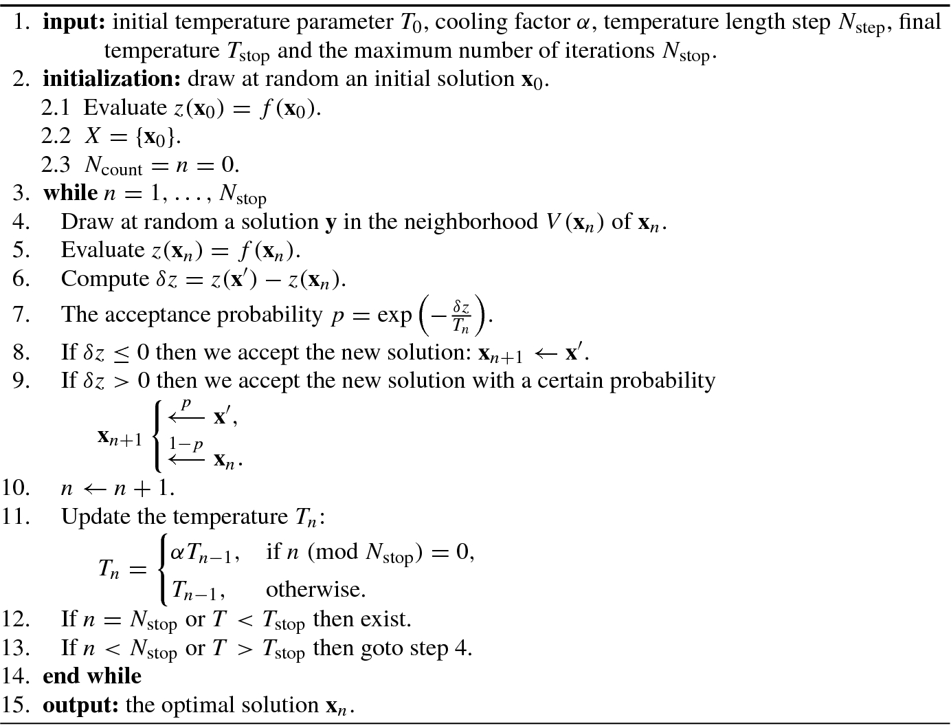
1. 1.
   Decision Rule: In this rule, when moving from a current solution (or state) x _i to the new solution x ^′, the cost criterion is defined as

   

   (9.5.2)
    
2. 2.

   Neighborhood V (x) is defined as a set of feasible solution close to x such that any solution satisfying the constraints of MOCO problems, D = {x : x ∈ LD, x ∈ B ⁿ} and LD = {x : Ax = b}, can be obtained after a finite number of moves.

    
3. 3.
   Typical parameters: Some simulated annealing-typical parameters must be fixed as follows:

   • The initial temperature parameter T ₀ or alternatively an initial acceptance probability p ₀;

   • The cooling factor α (α < 1) and the temperature length step N _step in the cooling schedule.

   • The stopping rule(s): final temperature T _stop and/or the maximum number of iterations without improvement N _stop.

    

Algorithm 9.4 shows a single-objective simulated annealing algorithm.

Algorithm 9.4 Single-objective simulated annealing [153]

Simulated annealing has the following two important features [88]:

1. 1.

   Annealing differs from iterative improvement in that the procedure need not get stuck since transitions out of a local optimum are always possible at nonzero temperature.

    
2. 2.

   Annealing is an adaptive form of the divide-and-conquer approach. Gross features of the eventual state of the system appear at higher temperatures, while fine details develop at lower temperatures.

    

9.5.2 Multiobjective Simulated Annealing Algorithm

Common ideas behind simulated annealing are [88, 91]:

• the concept of neighborhood;

• acceptance of new solutions with some probability;

• dependence of the probability on a parameter called the temperature; and

• the scheme of the temperature changes.

As comparison with single-objective simulated annealing, population-based simulated annealing (PSA) uses also the following ideas:

1. 1.

   Apply the concept of a sample (population) of interacting solutions from genetic algorithms [55] at each iteration in simulated annealing. The solutions are called generate solutions.

    
2. 2.

   In order to assure dispersion of the generated solutions over the whole set of efficient solutions, one must control the objective weights used in the multiple objective rules for acceptance probability in order to increase or decrease the probability of improving values of the particular objectives.

    

Different from the single-objective framework, in the multiple-objective framework, when comparing a new solution x ^′ with the current solution x _i according to K criteria z _k(x ^′, x _i), k = 1, …, K, three cases can obviously occur [153].

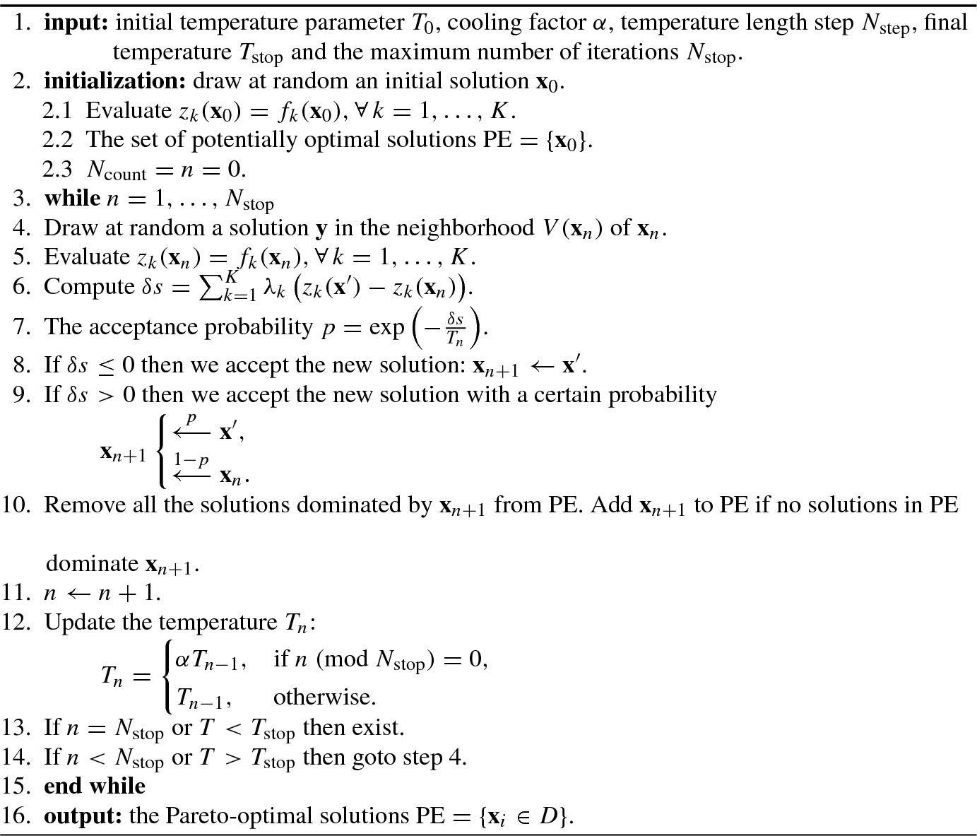
• If z _k(x ^′) ≤ z _k(x _n), ∀ k = 1, …, K then the move from x _i to x ^′ is an improvement with respect to all the objective δz _k(x ^′, x _n) = z _k(x ^′) − z _k(x _n) ≤ 0, ∀k = 1, …, K. Therefore, x ^′ is always accepted (p = 1).

• An improvement and a deterioration can be simultaneously observed on different cost criteria δz _k < 0 and . The first crucial point is how to define the acceptance probability p.

• When all cost criteria are deteriorated: ∀k, δz _k ≥ 0 at least one strict inequality, a probability p to accept x ^′ instead of x _i must be calculated. Let

  

  (9.5.3)

  For the computation of the probability p, the second crucial point is how to compute the “distance” between z(x ^′) and z(x _i).

To overcome the above two difficulties, Ulungu et al. [153] proposed a criterion scalarizing approach in 1999.

Define the probability from x _i to x ^′ with respect to the kth criterion as follows:

(9.5.4)

Then, the global acceptance probability p can be determined by

(9.5.5)

where Π = (π ₁, …, π _K) is an aggregation of K criteria π _k.

The most intuitive criterion scalarizing functions t(Π, λ) are the product function

(9.5.6)

and the minimum function

(9.5.7)

In order to compute the distance between two solutions for each individual and then to evaluate the acceptance probability of the move from x _i to x ^′ with respect to this particular criterion, an efficient criterion scalarizing approach is to choose the acceptance probability given by

(9.5.8)

Here δs = s(z(x ^′, λ)) − s(z(x _i, λ)) may take one of the following two forms:

• Weighed sum:

  

  (9.5.9)

  where

  

  (9.5.10)

  An equivalent alternative is given by Engrand [39]

  

  (9.5.11)
• Weighed Chebyshev norm L _∞:

  

  (9.5.12)

  where are the cost (criterion) values of the ideal point .

It is easily shown [153] that the global acceptance probability p in (9.5.8) is just a most intuitive scalarizing function, i.e., p = t(Π, λ).

Due to conflicting multiple objectives, a good algorithm for solving multiobjective optimization problems needs to have the following four important properties [114].

• Searching precision: Because of problem complexity of multiobjective optimization, the algorithm finds hardly the Pareto-optimal solutions, and hence it must find the possible near solutions to the optimal solutions set.

• Searching-time: The algorithm must find the optimal set efficiently during searching-time.

• Uniform probability distribution over the optimal set: The found solutions must be widely spread, or uniformly distributed over the real Pareto-optimal set rather than converging to one point because every solution is important in multiobjective optimization.

• Information about Pareto frontier: The algorithm must give as much information as possible about the Pareto frontier.

A multiobjective simulated annealing algorithm is shown in Algorithm 9.5.

Algorithm 9.5 Multiobjective simulated annealing [153]

It is recognized (see, e.g., [114]) that simulated annealing for multiobjective optimization has the following properties.

1. 1.

   By using the concepts of Pareto optimality and domination, high searching precision can be achieved by simulated annealing.

    
2. 2.

   The main drawback of simulated annealing is searching-time, as it is generally known that simulated annealing takes long time to find the optimum.

    
3. 3.

   An interesting advantage of simulated annealing is its uniform probability distribution property as it is mathematically proved [50, 104] that it can find each of the global optima with the same probability in a scalar finite-state problem.

    
4. 4.

   For multiobjective optimization, as all the Pareto solutions have different cost vectors that have a trade-off relationship, a decision maker must select a proper solution from the found Pareto solution set or sometimes by interpolating the found solutions.

    

Therefore, in order to apply simulated annealing in multiobjective optimization, one must reduce searching-time and effectively search Pareto optimal solutions. It should be noted that any solution in the set PE of Pareto-optimal solutions should not be dominated by other(s), otherwise any dominated solution should be removed from PE. In this sense, Pareto solution set should be the best nondominated set.

9.5.3 Archived Multiobjective Simulated Annealing

In multiobjective simulated annealing (MOSA) algorithm developed by Smith et al. [145], the acceptance of a new solution x is determined by its energy function. If the true Pareto front is available, then the energy of a particular solution x is calculated as the total energy of all solutions that dominates x. In practical applications, as the true Pareto front is not available all the time, one must estimate first the Pareto front F ^′ which is the set of mutually nondominating solutions found thus far in the process. Then, the energy of the current solution x is the total energy of nondominating solutions. These nondominating solutions are called the archival nondominating solutions or nondominating solutions in Archive.

In order to estimate the energy of the Pareto front F ^′, the number of archival nondominated solutions in the Pareto front should be taken into consideration in MOSA. But, this is not done in MOSA.

By incorporating the nondominating solutions in the Archive, one can determine the acceptance of a new solution. Such an MOSA is known as archived multiobjective simulated annealing (AMOSA), which was proposed by Bandyopadhyay et al. in 2008 [7], see Algorithm 9.6.

Algorithm 9.6 Archived multiobjective simulated annealing (AMOSA) algorithm [7]

The following parameters need to be set a priori in Algorithm 9.6.

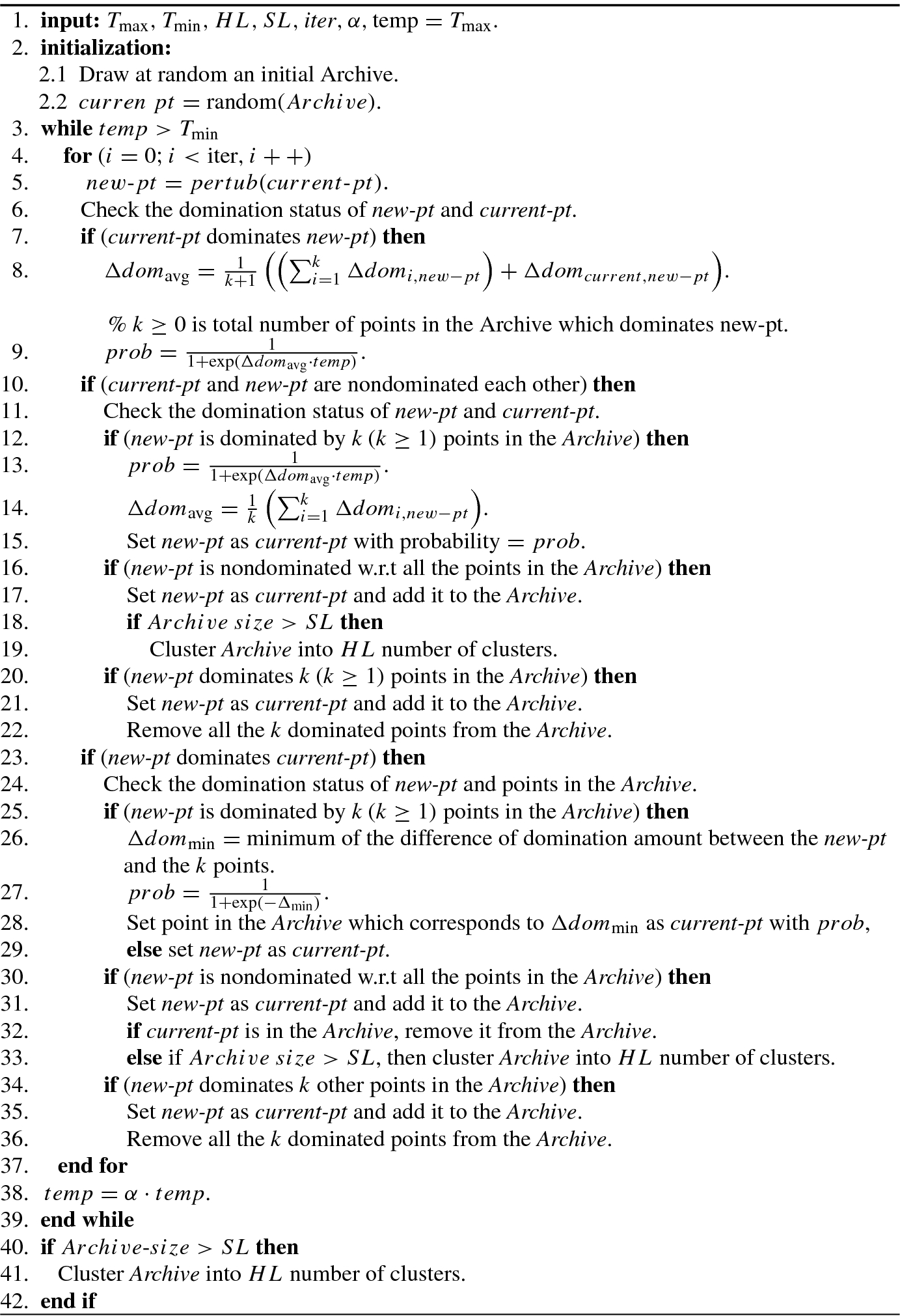
• HL: The maximum size of the Archive on termination. This set is equal to the maximum number of nondominated solutions required by the user;

• SL: The maximum size to which the Archive may be filled before clustering is used to reduce its size to HL;

• : Maximum (initial) temperature, : Minimal (final) temperature;

• iter: Number of iterations at each temperature;

• α: The cooling rate in SA.

Let denote the decision variable vector that simultaneously maximizes the objective values , while satisfying the constraints, if any. In maximization problems, a solution is said to dominate if and only if

(9.5.13)

(9.5.14)

Among a set of solutions P, the nondominated set P ^′ of solutions are those that are not dominated by any member of the set P. The nondominated set of the entire search space S is the globally Pareto-optimal set.

At a given temperature T, a new state s is selected with a probability

(9.5.15)

where q is the current state, whereas E(q, T) and E(s, T) are the corresponding energy values of q and s, respectively.

One of the points, called current-pt, is randomly selected from Archive as the initial solution at temperature . The current-pt is perturbed to generate a new solution called new-pt. The domination status of new-pt is checked with respect to the current-pt and solutions in Archive.

Depending on the domination status between current-pt and new-pt, the new-pt is selected as the current-pt with different probabilities. This process constitutes the core of Algorithm 9.6, see Step 4 to Step 37.

9.6 Genetic Algorithm

A genetic algorithm (GA) is a metaheuristic algorithm inspired by the process of natural selection. Genetic algorithms are commonly used to generate high-quality solutions to optimization and search problems by relying on bio-inspired operators such as mutation, crossover, and selection.

In a genetic algorithm, a population of candidate solutions (called individuals, creatures, or phenotypes) to an optimization problem is evolved toward better solutions. Each candidate solution has a set of properties (its chromosomes or genotype) which can be mutated and altered; traditionally, solutions are represented in binary as strings of 0s and 1s, but other encodings are also possible.

The evolution is an iterative process: (a) It usually starts from a population of randomly generated individuals. The population in each iteration is known as a generation. (b) In each generation, the fitness of every individual in the population is evaluated. The fitness is usually the value of the objective function in the optimization problem being solved. (c) The fitter individuals are stochastically selected from the current population, and each individual’s genome is modified (recombined and possibly randomly mutated) to form a new generation. (d) This new generation of candidate solutions is then used in the next iteration of the algorithm. (e) The algorithm terminates when either a maximum number of generations has been produced, or a satisfactory fitness level has been reached for the population.

9.6.1 Basic Genetic Algorithm Operations

The genetic algorithm consists of encoded chromosome, fitness function, reproduction, crossover, and mutation operations generally.

A typical genetic algorithm requires three important concepts:

• a genetic representation of the solution domain,

• a fitness function to evaluate the solution domain, and

• a notion of population. Unlike traditional search methods, genetic algorithms rely on a population of candidate solutions.

A genetic algorithm (GA) is a search technique used for finding true or approximate solutions to optimization and search problems. GAs are a particular class of evolutionary algorithms (EAs) that use inheritance, mutation, selection, and crossover (also called recombination) inspired by evolutionary biology.

GAs encode the solutions (or decision variables) of a search problem into finite-length strings of alphabets of certain cardinality. Candidate solutions are called individuals, creatures, or phenotypes. An abstract representation of individuals is called chromosomes, the genotype or the genome, the alphabets are known as genes and the values of genes are referred to as alleles. In contrast to traditional optimization techniques, GAs work with coding of parameters, rather than the parameters themselves.

One can think of a population of individuals as one “searcher” sent into the optimization phase space. Each searcher is defined by his genes, namely his position inside the phase space is coded in his genes. Every searcher has the duty to find a value of the quality of his position in the phase space.

To evolve good solutions and to implement natural selection, a measure is necessary for distinguishing good solutions from bad solutions. This measure is called fitness.

Once the genetic representation and the fitness function are defined, at the beginning of a run of a genetic algorithm a large population of random chromosomes is created. Each decoded chromosome will represent a different solution to the problem at hand.

When two organisms mate they share their genes. The resultant offspring may end up having half the genes from one parent and half from the other. This process is called recombination. Very occasionally a gene may be mutated.

Genetic algorithms are a way of solving problems by mimicking the same processes mother nature uses. They use the same combination of selection, recombination (i.e., crossover), and mutation to evolve a solution to a problem.

Chromosome Code

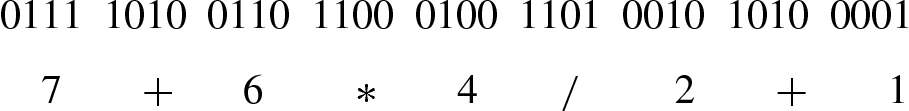
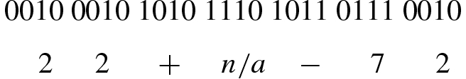
Each chromosome is made up of a sequence of genes from certain alphabet which can consist of binary digits (0 and 1), floating-point numbers, integers, symbols (i.e., A, B, C, D), etc.

In binary gene representation, a possible solution needs to be encoded as a string of bits (i.e., a chromosome), and these bits need to represent all the different characters available to the solution. For example, four bits are required to represent the range of characters used:

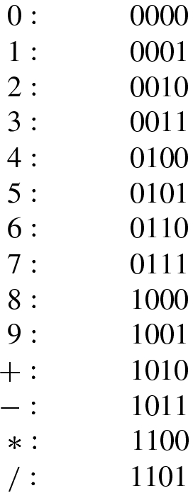
This shows all the different genes required to encode the problem as described. The possible genes 1110, 1111 will remain unused and will be ignored by the algorithm if encountered.

A string of four bits “7 + 6 ∗ 4 / 2 + 1” would be represented by nine genes as follows:

These genes are all strung together to form the chromosome:

Because the algorithm deals with random arrangements of bits it is often going to come across a string of bits like this:

Decoded, these bits represent:

Fitness Selection

To evolve good solutions and to implement natural selection, we need a measure for distinguishing good solutions from bad solutions. In essence, the fitness measure must determine a candidate solution’s relative fitness, which will subsequently be used by the GA to guide the evolution of good solutions. This is one of the characteristics of the GA: it only uses the fitness of individuals to get the relevant information for the next search step.

To assign fitness, Hajela and Lin [61] proposed a weighed-sum method: Each objective is assigned a weight w _i ∈ (0, 1) such that ∑_iw _i = 1, and the scalar fitness value is then calculated by summing up the weighted objective values w _if _i(x). To search multiple solutions in parallel, the weights are not fixed but coded in the genotype so that the diversity of the weight combinations is promoted by phenotypic fitness sharing [61, 169]. As a consequence, the fitness assignment evolves the solutions and weight combinations simultaneously.

Reproduction [164]

Individuals are selected through a fitness-based process, where fitter individuals with lower inferior value are typically more likely to be selected. On the one hand, excellent individuals must be reserved to avoid too random search and low efficiency. On the other hand, these high-fitness individuals are not expected to over breed, avoiding the premature convergence of the algorithm. For simplicity and efficiency, an elitist selection strategy is employed. First, the individuals in the population p(t) are sorted from small to large according to the inferior value. Then the former 1∕10 of the sorted individuals are directly selected into the crossover pool. The remaining 9∕10 of individuals are gained by random competitions of all individuals in the population.

Crossover and Mutation

Crossover is a unique feature of the originality of GA in evolutionary algorithms. Genetic crossover is a process of genetic recombination that mimics sexual reproduction in nature. Its role is to inherit the original good genes to the next generation of individuals and to generate new individuals with more complex genetic structures and higher fitness value.

The improved crossover probability P _ci of the ith individual is tuned adaptively as

(9.6.1)

where P _ci is the crossover probability of the GA, r _i is the inferior value of the individual, is the maximum inferior value, and r _avg is the average inferior value of the population.

By the crossover rate, it is simply the chance that two chromosomes will swap their bits. A good value for this is around 0.7. Crossover is performed by selecting a random gene along the length of the chromosomes and swapping all the genes after that point. For example, given two chromosomes

If choosing a random bit along the length, say at position 9, and swap all the bits after that point, then we have

It is seen from Eq. (9.6.1) for crossover probability that when the individual fitness value of the participating crossover is lower than the average fitness value of the population, i.e., the individual is a poor performing individual, a large crossover probability is adopted for it. When the individual fitness value of the crossover is higher than the average fitness value, i.e., the individual has excellent performance, then a small crossover probability is used to reduce the damage of the crossover operator to the better performing individual.

When the fitness values of the offspring generated by the crossover operation are no longer better than their parents, but the global optimal solution is not reached, the GA algorithm will occur premature convergence. At this time, the introduction of the mutation operator in the GA tends to produce good results.

Mutation in the GA simulates the mutation of a certain gene on the chromosome in the evolution of natural organisms in order to change the structure and physical properties of the chromosome.

On one hand, the mutation operator can restore the lost genetic information during population evolution to maintain individual differences in the population and prevent premature convergence. On the other hand, when the population size is large, for one to introduce moderate mutation after crossover operation, one can also improve the local search efficiency of the GA algorithm, thereby increasing the diversity of the population to reach the global domain of the search.

The improved mutation probability P _mi of the ith individual is tuned adaptively as

(9.6.2)

The mutation probability P _m of the population is adaptively changed according to the diversity of the current population as

(9.6.3)

where and are, respectively, the maximum and minimum inferior value of the individual, PopSize is the number of individuals, and P _m0 is the mutation probability of the program.

Mutation rate is the chance that one or more genes of a selected chromosome will be flipped (0 becomes 1, 1 becomes 0). Mutation probability is usually achieved using an adaptive selection:

(9.6.4)

Here k ₂ and k ₄ are equal to 0.5, and f is the fitness of the chromosome under mutation.

It can be seen from the expressions of P _ci in (9.6.1) and P _mi in (9.6.2) that

• When the individual fitness value is lower than the average fitness value of the population, namely the individual has a poor performance, one adopts a large crossover probability and mutation probability.

• If the individual fitness value is higher than the average fitness value, i.e., the individual’s performance is excellent, then the corresponding crossover probability and mutation probability are adaptively taken according to the fitness value.

• When the individual fitness value is closer to the maximum fitness value, the crossover probability and the mutation probability are smaller.

• If the individual fitness is equal to the maximum fitness value, then the crossover probability and the mutation probability are zero.

Therefore, individuals with optimal fitness values will remain intact in the next generation. However, this will allow individuals with the greatest fitness to rapidly multiply in the population, leading to premature convergence of the algorithm. Hence, this adjustment method is applicable to the population in the late stage of evolution, but it is not conducive to the early stage of evolution, because the dominant individuals in the early stage of evolution are almost in a state of no change, and the dominant individuals at this time are not necessarily optimized. The global optimal solution to the problem increases the likelihood of evolution to a locally optimal solution. To overcome this problem, we can use the default crossover probability p _c = 0.8 and the default mutation probability p _m = 0.001 for each individual, so that the crossover probability and mutation probability of individuals with good performance in the population are no longer zero.

9.6.2 Genetic Algorithm with Gene Rearrangement Clustering

Genetic clustering algorithms have a certain degree of degeneracy in the evolution process. The degeneracy problem is mainly caused by the non-one-to-one correspondence between the solution space of the clustering problem and the genetic individual coding in the evolution process [127].

The degeneracy of the evolutionary process usually causes the algorithm to search the local solution space repeatedly. Therefore, the search efficiency of the genetic clustering algorithm can be improved by avoiding the degeneracy of the evolution process.

To illustrate how the degeneracy occurs, consider a clustering problem in which a set of patterns is grouped into K clusters so that patterns in the same cluster are similar and differentiate from those of other clusters in some sense.

Denote two chromosomes as

(9.6.5)

(9.6.6)

with , and x is called a referenced vector. Let P ₁ = {1, …, K} be a set of indexes of {x ₁, …, x _K} and P ₂ = ∅. Consider the rearrangement of P ₁ to P ₂:

•   for i = 1 to K do

•    ,

•    P ₁ = P ₁∖k and P ₂(i) = k.

•   end for

Then, the elements of P ₂ will be a permutation of that of P ₁, and y will be rearranged according to P ₂, i.e.,

(9.6.7)

Definition 9.31 (Gene Rearrangement [16])

If x and y are two chromosomes in gene representation, and the elements of y are rearranged according to the indexes in P ₂ to get a new vector whose elements are given by

(9.6.8)

then the new chromosome is called the gene rearrangement of the original chromosome y.

The genetic algorithm with gene rearrangement (GAGR) clustering algorithm is given in Algorithm 9.7.

Algorithm 9.7 Genetic algorithm with gene rearrangement (GAGR) clustering algorithm [16]

The following are the illustration of the (GAGR) steps [16].

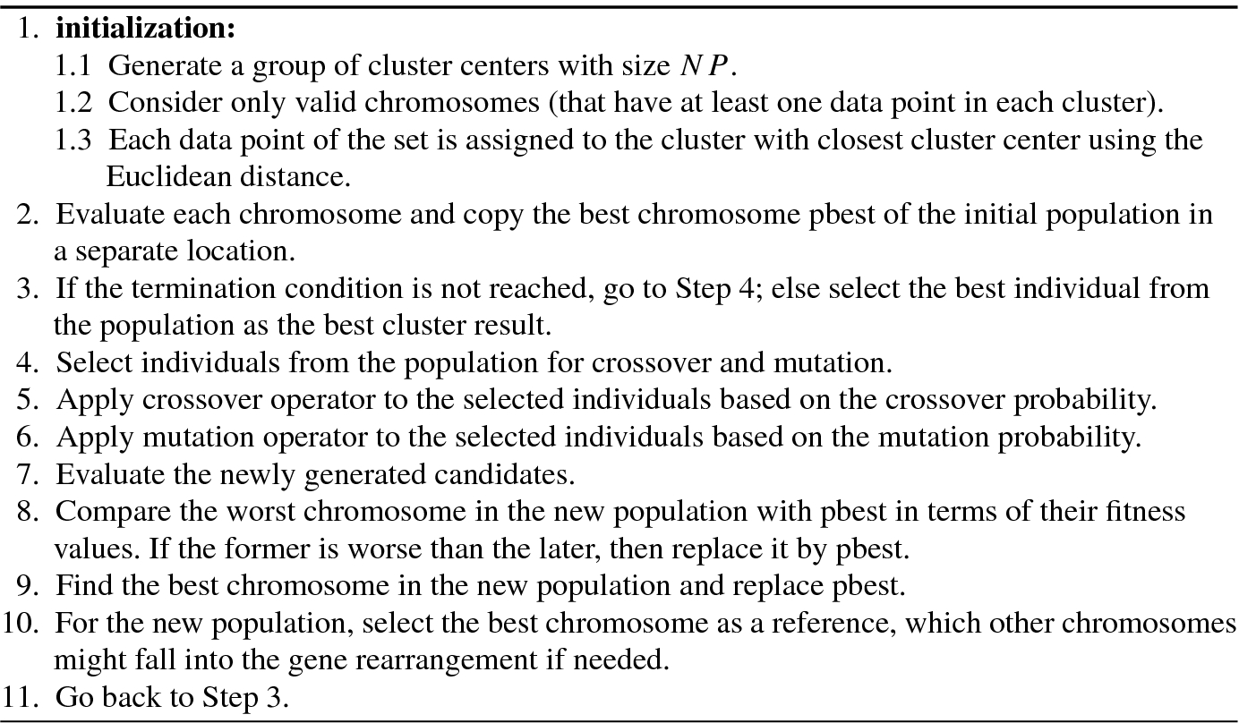
1. 1.
   Chromosome representation: Extensive experiments comparing real-valued and binary GAs indicate [102] that the real-valued GA is more efficient in terms of CPU time. In real-valued gene representation, each chromosome constitutes a sequence of cluster centers, i.e., each chromosome is described by M = N ⋅ K real-valued numbers as follows:

   

   (9.6.9)

   where N is the dimension of the feature space and K is the number of clusters; and the first N elements denote the first cluster center, the following N elements denote the second cluster center, and so forth.

    
2. 2.

   Population initialization: In GAGR clustering algorithm, an initial population of size N can be randomly generated and K data points randomly chosen from the data set, but on the condition that there are no identical points to form a chromosome, presenting the K cluster centers. This process is repeated until NP chromosomes are generated. Only valid strings (i.e., those that have at least one data point in each cluster) are considered to be included in the initial population.

   After the population initialization, each data point is assigned to the cluster with closest cluster center using the following equation:

   

   (9.6.10)

   where m _k is the center of the kth cluster.

    
3. 3.
   Fitness function: The fitness function is used to define a fitness value to each candidate solution. A common clustering criterion or quality indicator is the sum of squared error (SSE) measure, defined as

   

   (9.6.11)

   where x ∈ C _i is a data point assigned to that cluster. This measure computes the cumulative distance of each pattern from its cluster center of each cluster individually, and then sums those measures over all clusters. If this measure is small, then the distances from patterns to cluster centers are all small and the clustering would be regarded favorably. It is interesting to note that SSE has a theoretical minimum of zero, which corresponds to all clusters containing only a single data point. Then the fitness function of the chromosome is defined as the inverse of SSE, i.e.,

   

   (9.6.12)

   This fitness function will be maximized during the evolutionary process and lead to minimization of the SSE.

    
4. 4.
   Evolutionary operators:

   • Crossover: Let x and y be two chromosomes to be crossed, then the heuristic crossover is given by

     

     (9.6.13)
     

     (9.6.14)

     where r = U(0, 1) with U(0, 1) being a uniform distribution on interval [0, 1] and x is assumed to be better than y in terms of the fitness.

   • Mutation: Let and be the minimum and maximum fitness values in the current population, respectively. For an individual with fitness value f, a number δ ∈ [−R, +R] is generated with uniform distribution, where R is given by Bandyopdhyay and Maulik [5]:

     

     (9.6.15)
     If the minimum and maximum values of the data set along the ith dimension (i = 1, …, N) are and , respectively, then after mutation the ith element of the individual is given by Bandyopdhyay and Maulik [5]:

     

     (9.6.16)
    

One key feature of gene rearrangement is to avoid the degeneracy resulted by the representations used in many clustering problems. The degeneracy mainly arises from a non-one-to-one correspondence between the representation and the clustering result. To illustrate this degeneracy, let m ₁ = [1.1, 1.0, 2.2, 2.0, 3.4, 1.2] and m ₂ = [3.2, 1.4, 1.8, 2.2, 0.5, 0.7] represent, respectively, two clustering results of a two-dimensional data set with three cluster centers in one generation. If m ₁ is selected as the referenced vector, then m ₂ becomes after the gene rearrangement described by Definition 9.31.

Figure 9.3 provides a crossover results of m ₁ and .

Fig. 9.3

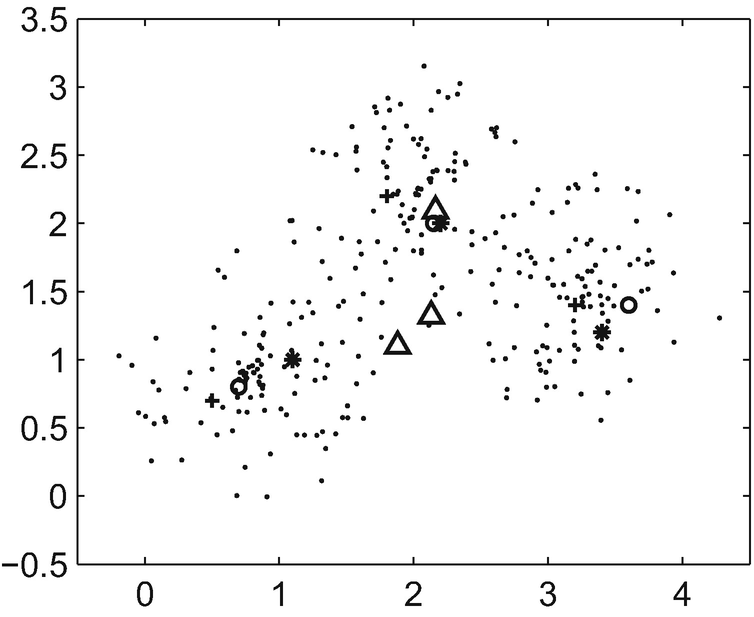
Illustration of degeneracy due to crossover (from [16]). Here, asterisk denotes three cluster centers (1.1, 1.0), (2.2, 2.0), (3.4, 1.2) for chromosome m ₁, +  denotes three cluster centers (3.2, 1.4), (1.8, 2.2), (0.5, 0.7) for the chromosome m ₂, open triangle denotes the chromosome obtained by crossing m ₁ and m ₂, and open circle denotes the chromosome obtained by crossing m ₁ and with three cluster centers (0.5, 0.7), (1.8, 2.2), (3.2, 1.4)

From Fig. 9.3 we can see that the performance of the chromosome marked by triangles in the figure directly obtained from crossing m ₁ and m ₂ is poor as two of the three clusters are very close, producing some confusion, while the chromosome marked by circles in the figure obtained from m ₁ and with gene rearrangement is more efficient because of no confusion between any pair of clusters.

Since there is a one-to-one correspondence between the representation and the clustering result through the gene rearrangement, there is no degeneracy, which makes the GAGR algorithm more efficient than the classical GA.

9.7 Nondominated Multiobjective Genetic Algorithms

In generation-based evolutionary algorithms (EAs) or genetic algorithms (GAs), the selected individuals are recombined (e.g., crossover) and mutated to constitute the new population. A designer/user prefers the more incremental, steady-state population update, which selects (and possibly deletes) only one or two individuals from the current population and adds the newly recombined and mutated individuals to it. Therefore, the selection of one or two individuals is a key step in generation-based EAs or GAs.

9.7.1 Fitness Functions

In the fields of genetic programming and genetic algorithms, each design solution is commonly represented as a string of numbers (called a chromosome). After each round of testing or simulation, the designer’s goal is to delete the “n” worst design solutions, and to breed “n” new ones from the best design solutions. To this end, each design solution needs to be evaluated by a figure of merit in order to determine how close it was to meeting the overall specification. This merit usually uses the fitness function to the test or simulation.

A fitness function, as a single figure of merit, is a particular type of objective function, and is used in genetic programming and genetic algorithms to guide simulations towards optimal design solutions.

According to “survival of the fittest” mechanism, a GA evaluates directly a solution by the fitness value of the solution. The GA requires only the fitness function to satisfy the nonnegativeness. This feature makes the genetic algorithm has wide applicability. Since a feasible solution x ₁ ∈ X is said to (Pareto) dominate another solution x ₂ ∈ X, if f _i(x ₁) ≤ f _i(x ₂) for all indices i ∈{1, …, k} and f _j(x ₁) < f _j(x ₂) for at least one index j ∈{1, …, k}, the objective function f _i(x) can naturally be taken as the fitness function of a candidate solution x. However, in practical problems, the fitness function is not completely consistent with the objective function of the problem.

In GAs, fitness is the key indicator to describe the individual’s performance. Due to selecting the fittest based on fitness, it becomes the driving force of the genetic algorithm. From a biological point of view, the fitness is equivalent to the survival competition. The “survival” biological viability is of great significance in the genetic process. Mapping the objective function of an optimization problem to the individual’s fitness can be achieved by optimizing the objective function of the optimization problem in the process of group evolution. The function is also known as the evaluation function, which is a criterion for distinguishing good individuals from bad ones in a group according to the objective function. The fitness is always nonnegative. In any case, it is expected that the larger the fitness value, the better.

In the selection operation, there are two genetic algorithm deceptive problems:

• In the early stage of GA, some supernormal individuals are usually generated. These supernormal individuals will control the selection process due to their outstanding competitiveness, which affects the global optimization performance of the algorithm.

• At the later stage of GA, if the algorithm tends to converge, then the potential for continued optimization is reduced and a certain local optimum solution may be obtained due to the small difference in individual fitness in the population. Therefore, if the fitness function is not properly selected, it will result in more than the problem of deception. The choice of fitness function can be seen as significant for genetic algorithms.

9.7.2 Fitness Selection

EAs/GAs are capable of solving complicated optimization tasks in which an objective function will be maximized, where i ∈ I is an individual from the set of feasible solutions. A population is a multi-set of individuals which is maintained and updated as follows: one or more individuals are first selected according to some selection strategy. In generation-based EAs, the selected individuals are then recombined (e.g., via crossover) and mutated in order to constitute the new population. We prefer to select (and possibly delete) only one or two individuals from the current population and adds the newly recombined and mutated individuals to it. We are interested in finding a single individual of maximal objective value for difficult multimodal and deceptive problems.

The following are the two common selection schemes [77]:

1. 1.
   Standard Selection Scheme: This scheme selects all favor individuals of higher fitness, and has the following variants:

   • Linear Proportionate Selection: In this method, the probability of selecting an individual depends linearly on its fitness [69].

   • Truncation Selection: In this selection the fittest individuals are selected, usually with multiplicity to keep the population size fixed [109].

   • Ranking Selection: This selection orders the individuals according to their fitness. The selection probability is, then, a (linear) function of the rank [157].

   • Tournament Selection: This method selects the best out of individuals. It has primarily developed for steady-state EAs, but can be adapted to generation based EAs [4].

    
2. 2.

   Fitness Uniform Selection Scheme (FUSS): FUSS is based on the insight that one is not primarily interested in a population converging to maximal fitness but only in a single individual of maximal fitness. The scheme automatically creates a suitable selection pressure and preserves genetic fitness values, and should help to preserve population diversity.

    

All above four standard selection schemes have the property (and goal) to increase the average fitness of a population, i.e., to evolve the population toward higher fitness [77].

Define the difference or distance between two individuals f(i) and f(j) as [77]:

(9.7.1)

The distance is based solely on the fitness function, and is independent of the coding/representation and other problem details, and of the optimization algorithm (e.g., the genetic mutation and recombination operators), and can trivially be computed from the fitness values. If making the natural assumption that functionally similar individuals have similar fitness, then they are also similar with respect to the distance d. On the other hand, individuals with very different coding and even functionally dissimilar individuals may be d-similar.

Two individuals i and j are said to be 𝜖-similar if d(i, j) = |f(i) − f(j)|≤ 𝜖.

Let the lowest and highest fitness values in the current population be and , respectively.

The fitness uniform selection scheme is a two-stage uniform selection process [77]:

• Randomly select a fitness value f uniformly from the fitness values .

• Select an individual i ∈ P with fitness nearest to f, and add a copy to the population P, possibly after mutation and recombination.

The probability of selecting a specific individual is proportional to the distance to its nearest fitness neighbor. In a population with a high density of unfitting and low density of fitting individuals, the more fitting ones are effectively favored.

To distinguish good solutions (individuals) from bad solutions, we need to make the fitness selection of individuals.

The fitness selection is a mathematical model or a computer simulation, or even is a subjective function for choosing better solutions over worse ones. In order to guide the evolution of good solutions in GAs, the fitness of every individual in the population is evaluated, multiple individuals are stochastically selected from the current population (based on their fitness), and modified (recombined and possibly mutated) to form a new population. The new population is then used in the next iteration of the GA. This iteration process is repeated until either a maximum number of generations has been produced, or a satisfactory fitness level has been reached for the population. However, if the algorithm has terminated due to a maximum number of generations, a satisfactory solution may or may not have been reached.

In contrast, we may also preserve diversity through deletion rather than selection, because we delete those individuals with “commonly occurring” fitness values. This method is called fitness uniform deletion scheme (FUDS) whose role is to govern actively different parts of the solution space rather than to move the population as a whole toward higher fitness [77]. Thus, FUDS is at least a partial solution to the problem of having to set correctly a selection intensity parameter.

A common fitness selection method is the Goldberg’s non-inferior sorting method for selecting the superior individuals [54]. Let x _i(t) be an arbitrary individual in the population p(t) of tth generation, r _i(t) indicate the number of individuals non-inferior to x _i(t) in this population. Then, r _i(t) is defined as the inferior value of the individual x _i(t) in the population. Obviously, individuals with small inferior value are superior, and are close to the Pareto solutions. In the process of evolution, the whole population keeps approaching to the Pareto boundary.

9.7.3 Nondominated Sorting Genetic Algorithms

Different from single-objective optimization problems, the performance improvement of one objective is often inevitable at the cost of descending at least another objective in the multiobjective optimization problems. In other words, it is hard to identify a unique optimal solution but rather a family of optimal solutions called the Pareto-optimal front or nondominated set.

Multiobjective evolutionary algorithms (MOEAs) are a most popular approach to solving multiobjective optimization problems because MOEAs are able to find multiple Pareto-optimal solutions in one single run. Since it is not possible for a multiobjective optimization problem to have a single solution which simultaneously optimizes all objectives, an algorithm is of great practical value if it gives a large number of alternative solutions lying on or near the Pareto-optimal front.

Earlier practical GA, called Vector Evaluated Genetic Algorithm (VEGA), was developed by Schaffer in 1985 [141]. One of the problems with VEGA is its bias toward some Pareto-optimal solutions. A decision maker may want to find as many nondominated points as possible in order to avoid any bias toward such middling individuals.

The number of dominating points d(s, P(t)) is the number of points y from set P(t) that dominate point s, namely

(9.7.2)

The d(s, P(t)) measure favors solutions located in those areas where the better fronts are sparsely populated. When the population may consist of nondominated solutions only, the d(s, P(t)) selection scheme is never available.

Definition 9.32 (Niched Pareto Genetic Algorithm [74])

A niched Pareto genetic algorithm combines tournament selection and the concept of Pareto dominance. For two competing individuals and a comparison set consisting of other individuals picked at random from the population, if one of the competing individuals is dominated by any member of the set, and the other is not, then the latter is chosen as winner of the tournament. If both individuals are dominated or not dominated, then the result of the tournament is decided by sharing: the individual which has the least individuals in its niche is selected for reproduction.

The niched Pareto genetic algorithm was proposed by Horn et al. in 1994 [74].

Nondominated sorting genetic algorithm (NSGA) differs from a simple genetic algorithm only in how the selection operator works. The crossover and mutation operators remain as usual: the population is ranked on the basis of an individual’s nondomination before the selection is performed. The nondominated individuals present in the population are first identified from the current population, then all these individuals are assumed to constitute the first nondominated front in the population and assigned a large dummy fitness value. If some nondominated individuals are assigned to the same fitness value, then all these nondominated individuals have an equal reproductive potential. To maintain diversity in the population, these classified individuals are then shared with their dummy fitness values.

Let the parameter d(x _i, x _j) be the phenotypic distance between two individuals x _i and x _j in the current front, and σ _share be the maximum phenotypic distance allowed between any two individuals to become members of a niche.

Definition 9.33 (Sharing Function Value [146])

For two individuals x _i and x _j in the same front, their sharing function value, denoted by sh(x _i, x _j), is defined as

(9.7.3)

For example, is taken.

Definition 9.34 (Niche Count [56])

Given X = {x ₁, …, x _L} (the union of the parent and offspring populations) and σ (the niche radius). Then, the niche count of x ∈ X is defined by

(9.7.4)

Sharing is achieved by performing selection operation via degraded fitness values obtained by dividing the original fitness value of an individual by a quantity proportional to the number of individuals around it. This causes multiple optimal points to co-exist in the population. These shared nondominated individuals are ignored temporarily, and are then assigned a new dummy fitness value for keeping smaller than the minimum shared dummy fitness of the previous front. This process is continued until the entire population is classified into several fronts [146].

In multiobjective optimization genetic algorithm, the whole population is checked and all nondominated individuals are assigned rank 1. Other individuals are ranked according to the nondominance of them with respect to the rest of the population as follows. For an individual point, the number of points that strictly dominate the point in the population is first found. Then, the rank of that individual is assigned to be one more than that number. At the end of this ranking procedure, there could be a number of points having the same rank. The selection procedure then uses these ranks to select or delete blocks of points to form the mating pool.

Algorithm 9.8 shows the nondominated sorting genetic algorithm (NSGA) [146].

Algorithm 9.8 Nondominated sorting genetic algorithm (NSGA) [146]

9.7.4 Elitist Nondominated Sorting Genetic Algorithm

The nondominated sorting genetic algorithm (NSGA) proposed by Srinivas and Deb [146] uses nondominated sorting and sharing, and its main criticism are as follows [25]:

• High computational complexity of nondominated sorting: Computational complexity of ordinary nondominated sorting algorithm is O(kN ³), where k is the number of objectives and N is the population size.

• Lack of elitism: Elitism can speed up the performance of the GA significantly, and also can help to prevent the loss of good solutions once they have been found.

• Need for specifying the sharing parameter σ _share: A parameterless diversity preservation mechanism is desirable.

To overcome the three shortcomings mentioned above, a fast and elitist multi-objective genetic algorithm (NSGA-II) was proposed by Deb et al. in 2002 [25]. Evolutionary multiobjective algorithms apply biologically inspired evolutionary processes as heuristics to generate nondominated sets of solutions. However, it should be noted that the solutions returned by evolutionary multiobjective algorithms may not be Pareto optimal (i.e., globally nondominated), but the algorithms are designed to evolve solutions that approach the Pareto front and spread out to capture the diversity existing on the Pareto front for obtaining a good approximation of the Pareto front [108].

The NSGA-II features nondominated sorting and a (μ + μ) (μ is the number of solution vectors) selection scheme. The secondary ranking criterion for solutions on the same front is called crowding distance. For a solution, the crowding distance is defined as the sum of the side lengths of the cuboid through the neighboring solutions on the front. For extremal solutions it is defined as infinity. The crowding distance value of a solution depends on its neighbors and not directly on the position of the point itself.

At the end of one generation of NSGA-II, the size of the population is twice bigger than the original size. This bigger population is pruned based on the nondominated sorting [80].

The basic NSGA-II steps are as follows [108]:

1. 1.

   Randomly generate the first generation.

    
2. 2.

   Partition the parents and offspring of the current generation into k fronts F ₁, …, F _k, so that the members of each front are dominated by all members of better fronts and by no members of worse fronts.

    
3. 3.

   Calculate the crowding distance for each potential solution: for each front, sort the members of the front according to each objective function from the lowest value to the highest value. Compute the difference between the solution and the closest lesser solution and the closest greater solution, ignoring the other objective functions. Repeat for each objective function. The crowding distance for that solution is the average difference over all the objective functions. Note that the extreme solutions for each objective function are always included.

    
4. 4.
   Select the next generation based on nondomination and diversity:

   • Add the best fronts F ₁, …, F _j to the next generation until it reaches the target population size.

   • If part of a front, F _j+1, must be added to the generation to reach the target population size, sort the members from the least crowded to most crowded. Then add as many members as are necessary, starting with the least crowded.

    
5. 5.
   Generate offspring:

   • Apply binary tournament selection by randomly choosing two solutions and including the higher-ranked solution with a fixed probability 0.5–1.

   • Apply single-point crossover and the sitewise mutation to generate offspring.

    
6. 6.

   Repeat steps 2 through 5 for the desired number of generations.

    

9.8 Evolutionary Algorithms (EAs)

Optimization plays a very important role in engineering, operational research, information science, and related areas. Optimization techniques can be divided into two categories: derivative-based methods and derivative-free methods. As an important branch of derivative-free methods, evolutionary algorithms (EAs) have shown considerable success in solving optimization problems and attracted more and more attention.

Single objective evolutional algorithms are general purpose optimization heuristics inspired by Darwin’s principle of natural evolution. Starting with a set of candidate solutions (population), in each iteration (generation), the better solutions are selected (parents) according to their fitness (i.e., function values under the objective function) and used to generate new solutions (offspring) through recombining the information of two parents in a new way (crossover) or randomly modifying a solution (mutation). These offspring are then inserted into the population, replacing some of the weaker solutions (individuals) [13].

By iteratively selecting the better solutions and using them to create new candidates, the population “evolves,” and the obtained solutions become better and better adapted to the optimization problem at hand, just like in the nature, where the individuals become better and better adapted to their environment through evolution.

EAs have successfully employed on a wide variety of complex optimization problems because they can deal with almost arbitrarily complex objective functions and constraints, resulting into very few assumptions and not even requiring a mathematical description of the problem.

9.8.1 (1 + 1) Evolutionary Algorithm

The most simple single objective evolutionary algorithm is called (1 + 1) evolutionary algorithm or (1 + 1) EA. The basic idea and steps of (1 + 1) EA are as follows [35]:

1. 1.

   The size of the population is restricted to just one individual and does not use crossover.

    
2. 2.

   The current individual is represented as a bit string.

    
3. 3.

   Use bitwise mutation operator that flips each bit independently of the others with some probability p _m.

    
4. 4.

   The current bit string is replaced by the new one if the fitness of the current bit string is not superior to the fitness of the new string. This replacement strategy selects the best individual of one parent and one child as the new generation.

    

(1 + 1) EA is shown in Algorithm 9.9.

Algorithm 9.9 (1 + 1) evolutionary algorithm [35]

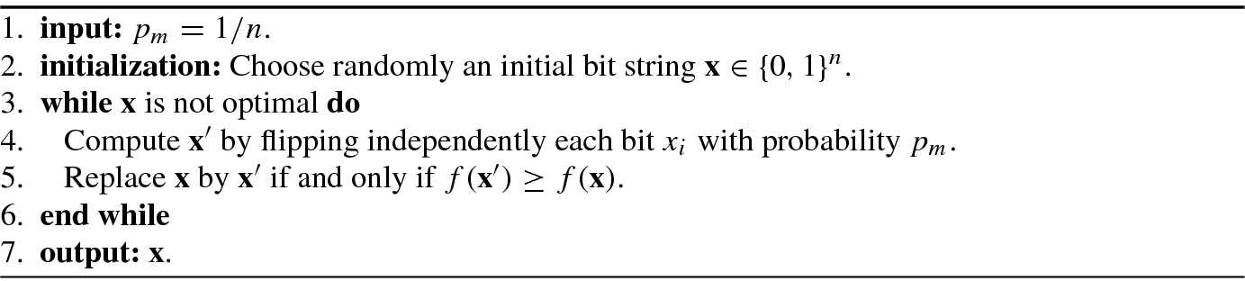
The different choices of selection, crossover, mutation, replacement, and concrete representation of the individuals offer a great variety of different EAs.

The combinatorial optimization problem can be described as follows: given a finite state space S and a function f(x), x ∈ S, find the solution

(9.8.1)

Assume x ^∗ is one state with the maximum function value, and . The EA for solving the combinatorial optimization problem can be described as follows:

1. 1.

   Initialization: generate, either randomly or heuristically, an initial population of 2N individuals, denoted by ξ ₀ = (x ₁, …, x _2N) (where N > 0 is an integer), and let k ← 0. For any population ξ _k, define .

    
2. 2.

   Generation: generate a new (intermediate) population by crossover and mutation (or any other operators for generating offspring), and denote it as ξ _k+1∕2.

    
3. 3.

   Selection: select and reproduce 2N individuals from populations ξ _k+1∕2 and ξ _k, and obtain another (new intermediate) population ξ _k+S.

    
4. 4.

   If , then stop; otherwise let ξ _k+1 = ξ _k+S and k ← k + 1, and go to step 2 to continue.

    

9.8.2 Theoretical Analysis on Evolutionary Algorithms

Several different methods are widely used in the theoretical analysis of EAs.

Fitness Partition

Fitness partition method is the very basic method, in which the objective fitness domain is partitioned into several levels.

Theorem 9.1 ([94])

Consider a maximization problem with fitness function . Suppose D can be partitioned into L subsets and for any solution x _i in subset i and x _j in subset j, we have f(x _i) < f(x _j) if i < j. In addition, subset L only contains optimal solution(s) of f. If an algorithm can jump from subset k to subset k + 1 or higher with probability at least p _k, then the total expected time for the algorithm to find the optimum satisfies

(9.8.2)

Drift Analysis

By considering the expected progress achieved in a single step at each search point, drift analysis [60, 66] can be used to analyze problems which are hard to be analyzed by fitness partition.

Assume x ^∗ is an optimal point, and let d(x, x ^∗) be the distance between two points x and x ^∗. If there are more than one optimal point (that is, a set S ^∗), then is used as the distance between individual x and the optimal set S ^∗. Denote the distance by d(x). Usually d(x) satisfies d(x ^∗) = 0 and d(x) > 0 for any x∉S ^∗.

Given a population X = {x ₁, …, x _2N}, let

(9.8.3)

which is used to measure the distance of the population to the optimal solution.

The drift of the random sequence {d(ξ _k);k = 0, 1, …} at time k is defined by

(9.8.4)

Define the stopping time of an EA as , which is the first hitting time on the optimal solution. The drift analysis focuses on the following question [66]: under what conditions of the drift can we estimate the expect first hitting time E[τ]?

A fitness function can be written as a polynomial [35]:

(9.8.5)

where coefficient .

Let the class of fitness functions f(s ₁, …, s _n) satisfy the condition

(9.8.6)

for any k = 1, …, n and fixed s ₁, …, s _k−1, s _k+1, …, s _n. This condition shows that if one “0” bit at any position flips into “1,” the fitness will increase, and thus (1, …, 1) is the unique maximum point.

Theorem 9.2 ([67])

For any fitness function (9.8.5) satisfying (9.8.6), the EA with mutation probability p _m = 1∕(2n) needs average steps to reach the optimal solution.

9.9 Multiobjective Evolutionary Algorithms

Multiobjective evolutionary algorithms (MOEAs) have been shown to be well-suited for solving multiobjective optimization problems (MOPs) with conflicting objectives as they can approximate the Pareto-optimal front with a population in a single run.

9.9.1 Classical Methods for Solving Multiobjective Optimization Problems

All classical methods for solving MOPs are to scalarize the objective vector into one scalar objective. The following are the three commonly used classical methods [146]:

1. 1.
   Method of objective weighting: multiple objective functions are combined into one overall objective function:

   

   (9.9.1)

   where w _i are fractional numbers (0 ≤ w _i ≤ l), and all weights are summed up to 1, or . In this method, the optimal solution is controlled by the weigh vector w = [w ₁, …, w _k]^T: the preference of each objective f _i(x) can be changed by modifying its corresponding weight w _i.

    
2. 2.
   Method of distance functions: the scalarization of objective vector f(x) = [f ₁(x), …, f _k(x)]^T is achieved by using a demand-level vector which has to be specified by the decision maker as follows:

   

   (9.9.2)

   where a Euclidean metric r = 2 is usually chosen, and the demand-level vector is individual optima of multiple objectives. The solution given by this method depends on the chosen demand-level vector. Arbitrary selection of a demand-level may be highly undesirable; a wrong demand-level will lead to a non-Pareto-optimal solution.

    
3. 3.
   Min-max formulation: this method attempts to minimize the relative deviations of the single objective functions from the individual optimum, namely it tries to minimize the objective conflict :

   

   (9.9.3)

   where Z _j(x) is calculated for nonnegative target optimal value as follows:

   

   (9.9.4)
    

Drawbacks of the above classical methods are: the optimization of the single objective may guarantee a Pareto-optimal solution, but results in a single-point solution. In real-world situations decision makers often need different alternatives in decision making. Moreover, if some of the objectives are noisy or have discontinuous variable space, then these methods may not work effectively.

Traditional search and optimization methods (such as gradient-based methods) are not available for extending to the multiobjective optimization because their basic design precludes the consideration of multiple solutions. In contrast, population-based methods (such as single objective evolutionary algorithms) are well-suited for handling such situations due to their ability to approximate the entire Pareto front in a single run [20, 24, 110].

The basic difference between multiobjective EAs from single objective EAs is how they rank and select individuals in the conflicting performance measures or objectives, many real-life multiobjective problems must be optimized simultaneously to achieve a trade-off.

In case of single objective, individuals are naturally ranked according to this objective, and it is clear which individuals are best and should be selected as parents. However, if there are multiple objectives, ranking the individuals is no longer obvious. Most people probably agree that a good approximation to the Pareto front is characterized by the following metrics [13]:

• a small distance of the solutions to the true Pareto frontier (such as dominated sorting solutions),

• a wide range of solutions, i.e., an approximation of the extreme values (such as extreme solutions),

• a good distribution of solutions, i.e., an even spread along the Pareto frontier (such as solutions with a larger distance to other solutions).

MOEAs then rank individuals according to how much they contribute to the above goals.

In MOEAs, the ability to balance between convergence and diversity depends on the selection strategy that can be broadly classified as: Pareto dominance-based MOEAs (PDMOEAs), indicator-based MOEAs, and decomposition-based MOEAs [119].

Difficulties in handling multiobjective problems can be roughly classified into the following five categories [87].

1. 1.

   Difficulties in searching for Pareto-optimal solutions.

    
2. 2.

   Difficulties in approximating the entire Pareto front.

    
3. 3.

   Difficulties in the presentation of obtained solutions.

    
4. 4.

   Difficulties in selecting a single final solution.

    
5. 5.

   Difficulties in the evaluation of search algorithms.

    

Two major problems must be addressed when an evolutionary algorithm is applied to multiobjective optimization [171]:

• How to accomplish fitness assignment and selection, respectively, in order to guide the search towards the Pareto-optimal set.

• How to maintain a diverse population in order to prevent premature convergence and achieve a well distributed trade-off front.

9.9.2 MOEA Based on Decomposition (MOEA/D)

Consider the multiobjective optimization problem (MOP)

(9.9.5)

where x = [x ₁, …, x _n]^T is the decision (variable) vector, Ω is the decision (variable) space, is the objective space, and consists of m real-valued objective functions. If Ω is a closed and connected region in and all the objectives are continuous of x, then the above problem is known as a continuous MOP.

A point x ^∗∈ Ω is called (globally) Pareto optimal if there is no x ∈  Ω such that f(x) dominates f(x ^∗), i.e., f _i(x) dominates f _i(x ^∗) for each i = 1, …, m. The set of all the Pareto-optimal points is called the Pareto set. The set of all the Pareto objective vectors, , is called the Pareto front.

Decomposition is a basic strategy in traditional multiobjective optimization. But, general MOEAs treat a MOP as a whole, and do not associate each individual solution with any particular scalar optimization problem. A multiobjective evolutionary algorithm based on decomposition (called MOEA/D) [167] decomposes an MOP by scalarizing functions into a number of subproblems, each of which is associated with a search direction (or weight vector) and assigned a candidate solution.

The followings are the three approaches for converting the problem of approximation of the Pareto front of problem (9.9.5) into a number of scalar optimization problems [167].

1. 1.
   Weighted sum approach: Let λ = [λ ₁, …, λ _m]^T be a weight vector with λ _i ≥ 0, ∀i = 1, …, m and . Then, the optimal solution to the scalar optimization problem

   

   (9.9.6)

   is a Pareto-optimal point to the MOP (9.9.5).

    
2. 2.
   Tchebycheff approach: This approach [103] can convert the problem of a Pareto-optimal solution of (9.9.5) into the scalar optimization problem:

   

   (9.9.7)

   where z = [z ₁, …, z _m]^T is the reference point vector, i.e., for each i = 1, …, m, and each optimal solution of (9.9.7) is a Pareto-optimal solution of (9.9.5), and thus one is able to obtain different Pareto-optimal solutions by altering the weight vector λ. Therefore, the Tchebycheff scalar optimization subproblem can be defined as [167]:

   

   (9.9.8)

   where λ _i is a weight parameter for the ith objective, and is set to the current best fitness of the ith objective. Tchebycheff approach used in MOEA/D can decompose the original MOP into several scalar optimization subproblems in form of (9.9.8), which can be solved with any optimization method for single objective optimization.

    
3. 3.
   Boundary intersection (BI) approach: This approach solves the following scalar optimization subproblem:

   

   (9.9.9)

   The goal of the constraint z ^∗−f(x) = dλ is to push f(x) as high as possible so that it reaches the boundary of the attainable objective set. In order to avoid the equality constraint in (9.9.9), one can use a penalty method to deal with the constraint [167]:

   

   (9.9.10)

   where θ > 0 is a preset penalty parameter, and

   

   (9.9.11)

   

   (9.9.12)
    

Multiobjective evolutionary algorithm based on decomposition (MOEA/D), proposed by Zhang and Li [167], uses the Tchebycheff approach to convert the problem of a Pareto-optimal solution of (9.9.5) into the scalar optimization problem (9.9.8).

Let be a set of weight vectors and z ^∗ be a reference point. The problem of approximation of the PF of (9.9.5) can be decomposed into scalar optimization subproblems by using the Tchebycheff approach and the objective function of the ith subproblem is given by

(9.9.13)

where .

As g ^tc is continuous of λ, the optimal solution of g ^tc(x|λ ⁱ, z ^∗) should be close to that of g ^tc(x|λ ^j, z ^∗) if λ ⁱ and λ ^j are close to each other. This makes any information about these g ^tc’s with weight vectors close to λ ⁱ should be helpful for optimizing g ^tc(x|λ ⁱ, z ^∗). This is a basic idea behind MOEA/D.

Let N be the number of the subproblems considered in MOEA/D, i.e., consider a population of N points x ¹, …, x ^N ∈ Ω, where x ⁱ is the current solution to the ith subproblem.

In MOEA/D, a neighborhood of weight vector λ ⁱ is defined as a set of its closest weight vectors in {λ ¹, …, λ ^N}. The neighborhood of the ith subproblem consists of all the subproblems with the weight vectors from the neighborhood of λ ⁱ. The population is composed of the best solution found so far for each subproblem. Only the current solutions to its neighboring subproblems are exploited for optimizing a subproblem in MOEA/D.

MOEA/D algorithm is shown in Algorithm 9.10.

Algorithm 9.10 Multiobjective evolutionary algorithm based on decomposition (MOEA/D) [167]

However, MOEA/D with simulated binary crossover has the following two shortcomings [93].

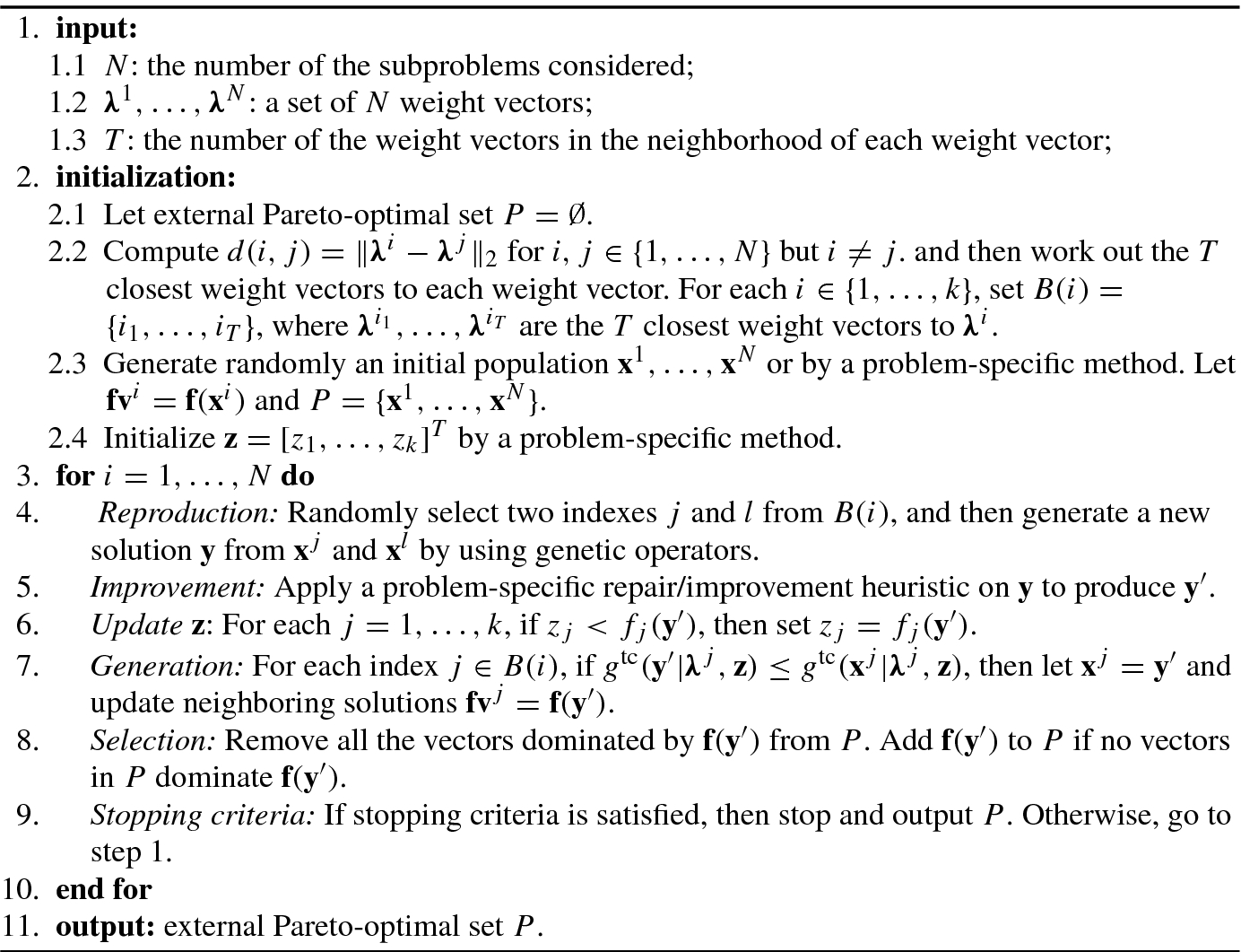
• The population in MOEA/D with simulated binary crossover may lose diversity, which is needed for exploring the search space effectively, particularly at the early stage of the search when applied to MOPs with complicated Pareto sets.

• The simulated binary crossover operator often generates inferior solutions in MOEAs.

To overcome these shortcomings, Li and Zhang [93] developed a version of MOEA/D based on differential evolution (DE), called MOEA/D-DE, which uses a differential evolution [124] operator and a polynomial mutation operator [24] to produce a new solution y = [y ₁, …, y _n]^T.

1. 1.
   Differential evolution operator: Generate a solution from three solutions , and selected randomly from P by a DE operator. The elements of are given by

   

   (9.9.14)

   for j = 1, …, n, where CR and F are two control parameters.

    
2. 2.
   Polynomial mutation operator: Generate y = [y ₁, …, y _n]^T from in the following way:

   

   (9.9.15)

   with

   

   (9.9.16)

   for j = 1, …, n, where rand is a uniform random number from [0, 1], the distribution index η and the mutation rate p _m are two control parameters, and a _j and b _j are the lower and upper bounds of the kth decision variable, respectively.

    

At each generation, MOEA/D-DE maintains the following:

• a population of points x ¹, …, x ^N ∈ Ω, where x ⁱ is the current solution to the ith subproblem;

• fv ¹, …, fv ^N, where fv ⁱ is the f-value of x ⁱ, i.e., fv ⁱ = [f ₁(x ⁱ), …, f _m(x ⁱ)]^T for each i = 1, …, N;

• z = [z ₁, …, z _m]^T, where z _i is the best value found so far for objective f _i.

MOEA/D-DE algorithm in [93] is shown in Algorithm 9.11.

Algorithm 9.11 MOEA/D-DE algorithm for Solving (9.9.5) [93]

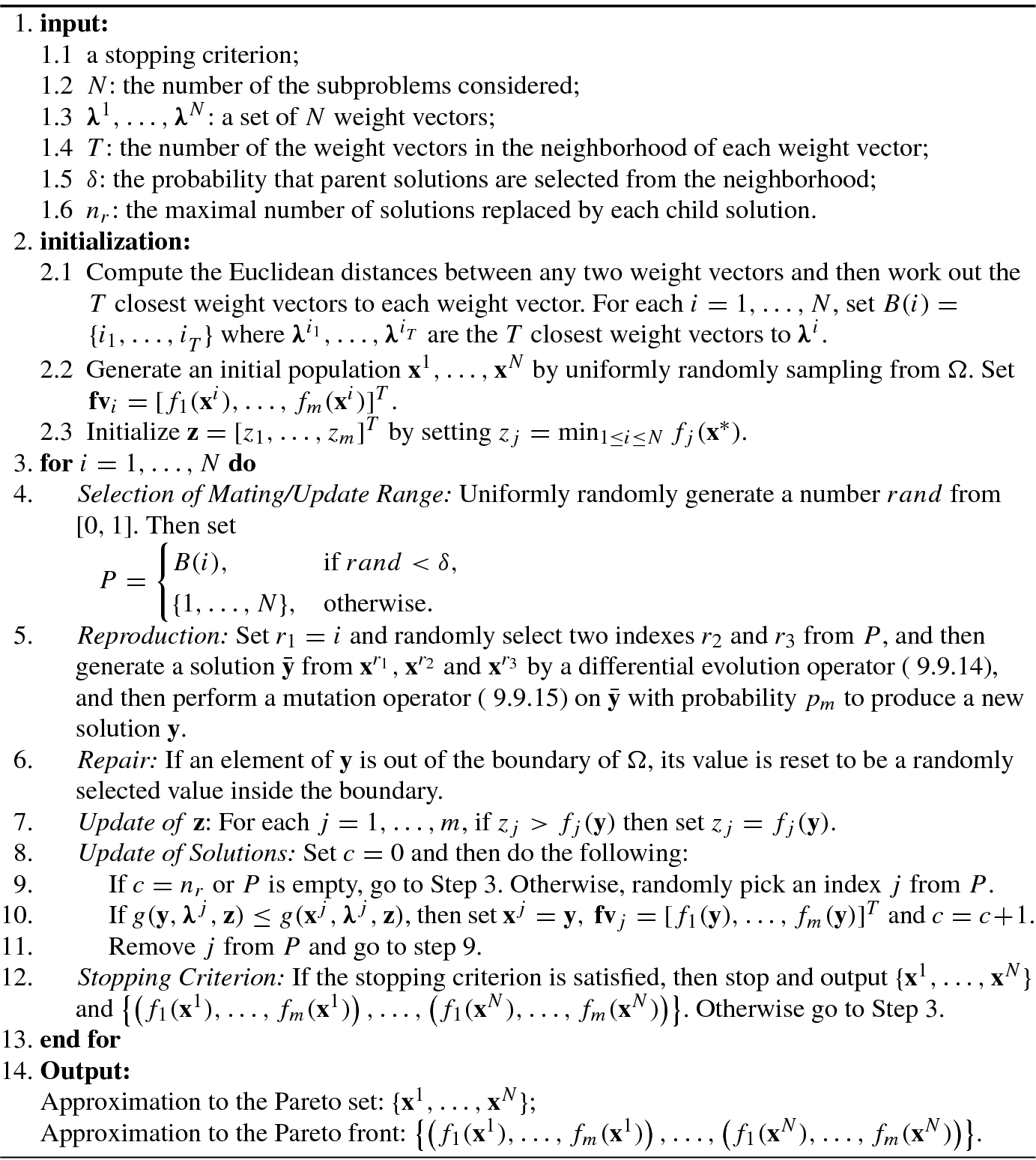
9.9.3 Strength Pareto Evolutionary Algorithm

It is widely recognized (e.g., see [45, 155]) that multiobjective evolutionary algorithms (MOEAs) can stochastically solve multiobjective optimization problems in an acceptable timeframe.

As their name implies, MOEAs are evolutionary computation based multiobjective optimization techniques.

General MOPs are mathematically defined as follows.

Definition 9.35 (General MOP [155])

In general, a multiobjective optimization (MOP) minimizes f(x) = [f ₁(x), …, f _k(x)] subject to g _i(x) ≤ 0, i = 1, …, m, x ∈ Ω. An MOP solution minimizes the components of a vector f(x), where x is an n-dimensional decision variable vector x = [x ₁, …, x _n]^T from some universe Ω.

Solution to MOP usually consists of both search (i.e., optimization) process and decision process. There are three decision making preferences [78]:

• A priori preference articulation (Decide → Search): Decision making combines the differing objectives into a scalar cost function. This effectively makes the MOP a single-objective prior to optimization.

• Progressive preference articulation (Search ↔ Decide): Decision making and optimization are intertwined. Partial preference information is provided upon which optimization occurs, providing an “updated” set of solutions for the decision making to consider.

• A posteriori preference articulation (Search → Decide): A decision making is presented with a set of Pareto optimal candidate solutions and chooses from that set. However, note that most MOEA researchers search for and present a set of nondominated vectors (PF _known) to the decision making.

As pointed out in [73] and [155], any practical MOEA implementation must include a secondary population composed of all Pareto-optimal solutions P _known(t) found so far during search. This is because the MOEA is a stochastic optimization, which does not guarantee that desirable solutions, once found, remain in the generational population until MOEA termination. For this end, one needs to make fitness assignment.

Let P denote the population and P′ be an external nondominated set. The fitness assignment procedure is a two-stage process [170].

1. 1.

   Each solution x _i ∈ P′ is assigned a real value s _i ∈ [0, 1), called strength; s _i is proportional to the number of population members for which x _i ≽x _j. Let n denote the number of individuals in P that are covered by x _i and assume N is the size of P. Then s _i is defined as . The fitness F _i of x _i is equal to its strength: F _i = s _i.

    
2. 2.
   The fitness of an individual j ∈ P is calculated by summing the strengths of all external nondominated solutions x _i ∈ P′ that cover x _j. The total fitness is added by 1 in order to guarantee that members of P′ have better fitness than members of P (note that fitness is to be minimized, i.e., small fitness values correspond to high reproduction probabilities):

   

   (9.9.17)
    

These are the following three main techniques used in MOEAs [170].

• Store the nondominated solutions in P′ found so far externally.

• Use the concept of Pareto dominance in order to assign scalar fitness values to individuals in P.

• Perform clustering to reduce the number of nondominated solutions stored in P without destroying the characteristics of the trade-off front.

Strength Pareto EA (SPEA) uses the following techniques for finding multiple Pareto-optimal solutions in parallel [170].

1. (a)

   It combines the above three techniques in a single algorithm.

    
2. (b)

   The fitness of an individual in P is determined only from the solutions stored in the external nondominated set P′; whether members of the population dominate each other is irrelevant.

    
3. (c)

   All solutions in the external nondominated set P′ participate in the selection.

    
4. (d)

   A niching method is provided in order to preserve diversity in the population P; this method is Pareto-based and does not require any distance parameter (like the niche radius for sharing).

    

Since SPEA uses a mixture of the three basic techniques in MOEAs in (a) and other three techniques (b)–(d), this MOEA method is a strength Pareto variant of MOEAs, and hence is named as SPEA.

Algorithm 9.12 shows the flow of the SPEA algorithm.

Algorithm 9.12 SPEA algorithm [170]

The average linkage method [107] can be used for the pruning by clustering in Step 5 in Algorithm 9.12. The average linkage method contains the following steps.

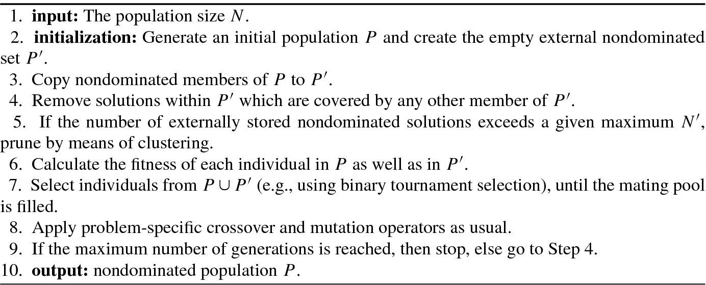
1. (1)

   Initialize cluster set C; each external nondominated point x _i ∈ P′ constitutes a distinct cluster: C =⋃_i{x _i}.

    
2. (2)

   If |C|≤ N′ , go to Step (5), else go to Step (3).

    
3. (3)
   Calculate the distance of all possible pairs of clusters. The distance d(c ₁, c ₂) of two clusters c ₁, c ₂ ∈ C is given as the average distance between pairs of individuals across the two clusters:

   

   (9.9.18)

   where |c _i| denotes the number of individuals in class c _i, i = 1, 2, the metric reflects the Euclidean distance between two individuals and , and is called as the Euclidean metric on the objective space.

    
4. (4)

   Determine two clusters c ₁ and c ₂ with minimal distance d(c ₁, c ₂); the chosen clusters amalgamate into a larger cluster C = C ∖{c ₁, c ₂}∪{c ₁ ∪ c ₂}. Go to Step (2).

    
5. (5)

   Compute the reduced nondominated set by selecting a representative individual per cluster. Use the centroid (the point with minimal average distance to all other points in the cluster) as representative solution.

    

Consider an improvement of SPEA, called SPEA2.

In multiobjective evolutionary optimization, the approximation of the Pareto-optimal set involves itself two (possibly conflicting) objectives: the distance to the optimal front is to be minimized and the diversity of the generated solutions is to be maximized (in terms of objective or parameter values). In this context, there are three fundamental issues when designing a multiobjective evolutionary algorithm [172]: fitness assignment, environmental selection, and mating selection.

Fitness Assignment

To avoid the situation that individuals dominated by the same archive members have identical fitness values, for each individual both dominating and dominated solutions are taken into account in SPEA2. Each individual i in the archive and the population P _t is assigned a strength value S(i), representing the number of solutions it dominates:

(9.9.19)

where |⋅| denotes the cardinality of a set, and the symbol >  corresponds to the Pareto dominance relation. Use the S(i) values to calculate the raw fitness value R(i) of an individual i as follows:

(9.9.20)

Remark 1

The raw fitness is determined by the strengths of its dominators in both archive and population in SPEA2, while SPEA considers only archive members in this context.

Remark 2

Fitness is to be minimized in SPEA2, i.e., R(i) = 0 corresponds to a nondominated individual, while a high R(i) value means that i is dominated by many individuals (which in turn dominate many individuals).

The raw fitness assignment provides a sort of niching mechanism based on the concept of Pareto dominance, but it may fail when most individuals do not dominate each other. To avoid this drawback, additional density information is incorporated to discriminate between individuals having identical raw fitness values. The density D(i) corresponding to i is defined by

(9.9.21)

where denotes the distance of i to its kth nearest neighbor in , and .

Finally, adding D(i) to the raw fitness value R(i) of an individual i yields its fitness F(i):

(9.9.22)

Environmental Selection

This selection involves which individuals in the population to keep during the evolution process. For this end, beside the population, an archive is necessary to contain a representation of the nondominated Pareto front among all solutions considered so far. During environmental selection, the first step is to copy all nondominated individuals having a fitness lower than one from archive and population to the archive of the next generation:

(9.9.23)

If the nondominated front fits exactly into the archive () the environmental selection step is completed. Otherwise, if the archive is too small (), then the best dominated individuals in the previous archive and population are copied to the new archive . This can be implemented by sorting the multi-set according to the fitness values and copy the first individuals i with F(i) ≥ 1 from the resulting ordered list to . Conversely, if the archive is too large () then an archive truncation procedure is invoked which iteratively removes individuals from until . In other words, the individual which has the minimum distance to another individual is chosen at each stage; if there are several individuals with minimum distance, the tie is broken by considering the second smallest distances and so forth.

Mating Selection

The pool of individuals at each generation is evaluated in a two stage process. First all individuals are compared on the basis of the Pareto dominance relation, which defines a partial order on this multi-set. Basically, the information which decides how each individual dominates, is dominated by or is indifferent to, is used to define a ranking on the generation pool. Afterwards, this ranking is refined by the incorporation of density information. Various density estimation techniques are used to measure the size of the niche in which a specific individual is located.

Algorithm 9.13 summarizes the improved strength Pareto evolutionary algorithm (SPEA2).

Algorithm 9.13 Improved strength Pareto evolutionary algorithm (SPEA2) [172]

The main differences of SPEA2 in comparison to SPEA are as follows [172].

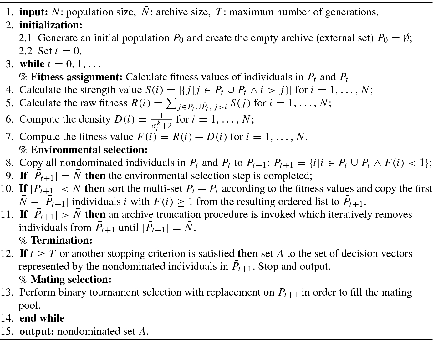
• An improved fitness assignment scheme is used, which takes for each individual into account how many individuals it dominates and it is dominated by.

• A nearest neighbor density estimation technique is incorporated which allows a more precise guidance of the search process.

• A new archive truncation method guarantees the preservation of boundary solutions.

9.9.4 Achievement Scalarizing Functions

Achievement scalarizing functions (ASFs), introduced by Wierzbicki [158], are denoted by which map (or scalarize) k objective functions to a scalar. The achievement scalarizing problem is given by

(9.9.24)

Certain properties of ASFs guarantee that scalarizing problem (9.9.24) yields Pareto-optimal solutions.

Definition 9.36 (Increasing Function [158])

An achievement scalarizing function is said to be

1. 1.

   Increasing: if for any for all i ∈{1, …, k}, then .

    
2. 2.

   Strictly increasing: if for any for all i ∈{1, …, k}, then .

    
3. 3.

   Strongly increasing: if for any for all i ∈{1, …, k} and y ¹ ≠ y ², then .

    

Clearly, any strongly increasing ASF is also strictly increasing, and any strictly increasing ASF is also increasing. The following theorems define necessary and sufficient conditions for an optimal solution of (9.9.24) to be (weakly) Pareto optimal.

Theorem 9.3 ([159, 160])

The necessary and sufficient conditions for an optimal solution being Pareto optimal are as follows.

1. 1.

   Let be strongly (strictly) increasing. If x ^∗∈ X is an optimal solution of problem (9.9.24), then x ^∗ is (weakly) Pareto optimal.

    
2. 2.

   If is increasing and the solution x ^∗∈ X of (9.9.24) is unique, then x ^∗ is Pareto optimal.

    

Theorem 9.4 ([103])

If is strictly increasing and x ^∗ ∈ X is weakly Pareto optimal, then it is a solution of (9.9.24) with the reference point f(x ^∗) and the optimal value of s _R is zero.

One example of the achievement scalarizing problems can be formulated as

(9.9.25)

(9.9.26)

where the term is called the augmentation term, in which ρ > 0 is a small constant, and z ^nad and z ^utopian are the nadir vector and utopian vectors, respectively. In the above problem, the parameter is the so-called reference point which represents objective function values preferred by the decision maker.

The following are the several most well-known ASFs [116].

1. 1.
   The strictly increasing ASF is of Chebyshev type:

   

   (9.9.27)

   where x ^∗ is a reference point, and λ is k-vector of nonnegative coefficients used for scaling purposes, that is, for normalizing objective functions of different magnitudes.

    
2. 2.
   The strongly increasing ASF is of augmented Chebyshev type:

   

   (9.9.28)

   where ρ > 0 is a small parameter.

    
3. 3.
   The additive ASF based on the L ₁ metric [137]:

   

   (9.9.29)
    
4. 4.
   The parameterized ASF: Let be a subset of N _k = {1, …, k} of cardinality q. The parameterized ASF is defined as follows [116]:

   

   (9.9.30)

   where q ∈ N _k and λ = [λ ₁, …, λ _k]^T, λ _i > 0, i ∈ N _k. Notice that

   • for ;

   • for ;

   • for .

   Here, “≅” means equality in the case where there exist no feasible solutions x ∈ X which strictly dominate the reference point, i.e., such that f _i(x) < f _i(x ^∗) for all i ∈ N _k.

    

The performance of the additive ASF can be described by the following two theorems.

Theorem 9.5 ([137])

Given problem (9.9.24) with ASF defined by (9.9.29), let f(x ^∗) be a reference point such that f(x ^∗) is not dominated by an objective vector of any feasible solution of problem (9.9.24). Also assume λ _i > 0 for all i ∈{1, …, k}. Then any optimal solution of problem (9.9.24) is a weakly Pareto-optimal solution.

Theorem 9.6 ([137])

Given problem (9.9.24) with ASF defined by (9.9.29) and any reference point f(x ^∗), and assume λ _i > 0 for all i ∈{1, …, k}. Then among the optimal solutions of problem (9.9.24) there exists at least one Pareto-optimal solution. If the optimal solution of problem (9.9.24) is unique, then it is Pareto optimal.

When adopting the parameterized ASF, the corresponding parameterized achievement scalarizing problem is given by Nikulin et al. [116]:

(9.9.31)

For any x ∈ X, denoting I _x = {i ∈ N _k : f _i(x ^∗) ≤ f _i(x)}, then the following two results are true:

Theorem 9.7 ([116])

Given problem (9.9.31), let f(x ^∗) be a reference point vector such that there exists no feasible solution whose image strictly dominates f(x ^∗). Also assume λ _i > 0 for all i ∈ N _k. Then, any optimal solution of problem (9.9.31) is a weakly Pareto-optimal solution.

Theorem 9.8 ([116])

Given problem (9.9.31), let f(x ^∗) be any reference point. Also assume λ _i > 0 for all i ∈ N _k. Then, among the optimal solutions of problem (9.9.31) there exists at least one Pareto-optimal solution.

Theorem 9.8 implies that the uniqueness of the optimal solution guarantees its Pareto optimality.

9.10 Evolutionary Programming

It is widely recognized [44] that evolutionary programming (EP) was first proposed as an approach to artificial intelligence. The EP has been applied with success to many numerical and combinatorial optimization problems.

9.10.1 Classical Evolutionary Programming

Consider a global minimization problem formalized as a pair (S, f), where with S being a bounded set on and f is an n-dimensional real-valued function. Our aim is to find a point such that is a global minimum on S, namely

(9.10.1)

where f is a bounded function which does not need to be continuous.

Optimization by EP can be summarized into two major steps:

• mutate the solutions in the current population;

• select the next generation from the mutated solutions and the current solutions.

There are the classical evolutionary programming (CEP) with self-adaptive mutation and the CEP without self-adaptive mutation. It is well-known (see, e.g., [3, 42, 165]) that the former usually performs better than the latter.

By Bäck and Schwefel [3], the CEP is implemented as follows (see also [165]).

1. 1.

   Initialization: Generate the initial population of μ individuals, and set k = 1. Each individual is taken as a pair of real-valued vectors (x _i, η _i) (i = 1, …, μ), where x _i are objective variables and η _i are standard deviations for Gaussian mutations (also called strategy parameters in self-adaptive evolutionary algorithms).

    
2. 2.

   Evaluation of fitness: Use the objective function f(x _i) to evaluate the fitness score for each individual (x _i, η _i), ∀ i = 1, …, μ.

    
3. 3.
   Self-adaptive mutation: Each parent (x _i(t − 1), η _i(t − 1)), i = 1, …, μ at the tth generation creates a single offspring (x _i(t), η _i(t)) at the tth generation:

   

   (9.10.2)

   

   (9.10.3)

   for i = 1, …, μ; j = 1, …, n. Here and denote the jth components of the parent vectors x _i(t − 1) and η _i(t − 1) at the (t − 1)th generations, respectively; and and are, respectively, the jth components of the offspring x _i(t) and η _i(t) at the tth generation; while N(0, 1) is a standard Gaussian distribution used for all j = 1, …, n, and N _j(0, 1) represents the standard Gaussian distribution used just for some given j. The factors are commonly set to and .

    
4. 4.

   Fitness for each offspring: Calculate the fitness of each offspring (x _i(t), η _i(t)), i = 1, …, μ.

    
5. 5.

   Pairwise comparison: Conduct pairwise comparison over the union of parents (x _i(t − 1), η _i(t − 1)) and offspring (x _i(t), η(t)) for all i = 1, …, μ. For each individual, opponents are chosen uniformly at random from all the parents and offspring. For each comparison, if the individual’s fitness is no smaller than the opponent’s, it receives a “win.”

    
6. 6.

   Selection: Select the μ individuals out of (x _i(t − 1), η _i(t − 1)) and (x _i(t), η _i(t)), that have the most wins to be parents of the next generation.

    
7. 7.

   Stopping criteria: Stop if the halting criterion is satisfied; otherwise, k = k + 1 and go to Step 3, and repeat the above steps.

    

The feature of CEP is to use the standard Gaussian mutation operator N _j(0, 1) in self-adaptive mutation (9.10.2).

9.10.2 Fast Evolutionary Programming

To speed up the convergence of the CEP, a fast evolutionary programming (FEP) was suggested by Yao et al. [165]. The one-dimensional Cauchy density function centered at the origin is defined by

(9.10.4)

where t > 0 is a scale parameter. The corresponding distribution function is

(9.10.5)

The variance of the Cauchy distribution is infinite.

The FEP is exactly the same as the CEP except for Gaussian mutation operator N _j(0, 1) in (9.10.2) which is replaced by Cauchy mutation operator as follows:

(9.10.6)

where C _j(0, 1) is a standard Cauchy random variable with the scale parameter t = 1 and is generated anew for each value of j.

The main difference between the FEP and CEP is: the CEP mutation equation (9.10.2) is a self-adaption controlled by the Gaussian distribution N _j(0, 1); while the FEP mutation equation (9.10.6) is a self-adaption controlled by the Cauchy random variable δ _i.

It is known [165] that Cauchy mutation is more likely to generate an offspring further away from its parent than Gaussian mutation due to its long flat tails. It is expected to have a higher probability of escaping from a local optimum or moving away from a plateau, especially when the “basin of attraction” of the local optimum or the plateau is large relative to the mean step size. Therefore, the FEP is expected to be faster than the CEP from viewpoint of convergence.

The basic steps of the FEP algorithm are described as follows [18].

1. 1.

   Generate an initial population of μ solutions (x _i, η _i), i ∈{1, …, μ}, and evaluate their fitness f(x _i).

    
2. 2.
   For every parent solution (x _i, η _i) in the population, create an offspring using

   

   where x _i(j), η _i(j) denote the jth components of the parent vectors x _i, η _i, and are the jth components of the offspring , respectively; while N(0, 1) is sampled from a standard Gaussian distribution for all j = 1, …, n, and N _j(0, 1) is sampled from an another standard Gaussian distribution just for some given j, while C _j(0, 1) is sampled from a standard Cauchy distribution for each i and j. The factors τ and τ ^′ are commonly set to and .

    
3. 3.
   For every parent solution (x _i, η _i) in the population, create another offspring using

   
    
4. 4.

   Evaluate the fitness of offspring solutions and .

    
5. 5.

   Perform pairwise tournaments over the union of parents (x _i, η _i) and offspring (i.e., and . For each solution in the union, q opponents are chosen uniformly at random from the union. For every tournament, if the fitness of the solution is no smaller than the fitness of the opponent, it is awarded a “win.” The total number of wins awarded to a solution (x _i, η _i) is denoted by win(x _i, η _i).

    
6. 6.

   Choose μ individual solutions from the union of parents and offspring at step 5. Chosen solutions will form the population of the next generation.

    
7. 7.

   Stop if the number of generations exceeds a predetermined number.

    

By performing on a number of benchmark problems, the experimental results show [165] that FEP with the Cauchy mutation operator C _j(0, 1) performs much better than CEP with the Gaussian mutation operator for multimodal functions with many local minima while being comparable to CEP in performance for unimodal and multimodal functions with only a few local minima.

A comparative study of applications of Cauchy and Gaussian mutation operators in electromagnetics reported in [70] and [72] was also observed that Cauchy mutation operator performs better than its Gaussian counterpart for a number of unconstrained or weakly constrained antenna optimization problems, but it performs relatively poor for highly constrained problems.

9.10.3 Hybrid Evolutionary Programming

Consider evolutionary programming for constrained optimization problems

(9.10.7)

where f and g ₁, …, g _r are functions on , and h ₁, …, h _m are functions on for m ≤ n and and x ∈ F ⊆ S. A vector x is called a feasible solution to the optimization problem (P) if and only if x satisfies the r inequality constraints g _i(x) ≤ 0, i = 1, …, r and m equality constraints h _j(x) = 0, j = 1, …, m. When the collection of feasible solutions is empty, x is said to be infeasible. The set defines the search space for x and the set F ⊆ S defines a feasible part of the search space S.

Use the cost function to evaluate a feasible solution, i.e.,

(9.10.8)

and define the constraint violation measure for the constraints as follows:

(9.10.9)

or

(9.10.10)

where |⋅| denotes an absolute value of the argument, and

(9.10.11)

is the magnitude of the violation of the ith constraint in (P), where 1 ≤ i ≤ r. Then,

(9.10.12)

defines the total evaluation of an individual x, where s is a penalty parameter of a positive for minimization or a negative constant for maximization. Clearly, Φ(x) can be interpreted as the error (for a minimization problem) or fitness (for a maximization problem) of an individual x to the optimization problem (P).

Therefore, the original constrained optimization problem (P) becomes the following unconstrained optimization problem:

(9.10.13)

where Φ _u(x) is defined by (9.10.9) or (9.10.10).

Different from CEP and FEP whose each individual is a two-tuples of real-valued vectors (x _i, η _i), Myung et al. [112, 113] proposed an EP to update a triplet of real-valued vectors , and named it as the hybrid evolutionary programming (HEP).

In HEP, , while and are the n-dimensional solution vector and its two corresponding strategy parameter vectors, respectively. Here and are initialized based on the specified search domains, , which may be imposed at the initialized stage.

HEP is named because of applying hybrid (Cauchy +  Gaussian) mutation operators as follows [71]:

(9.10.14)

(9.10.15)

(9.10.16)

(9.10.17)

for i = 1, …, n, where x _i(j), σ _i(j), and η _i(j) are the jth components of the vectors x _i, σ _i, and η _i, respectively. C _j(0, 1) in (9.10.14) and N _j(0, 1) in (9.10.14), (9.10.16), and (9.10.17) indicate that the random variables are generated anew for each value of j in each equation.

9.11 Differential Evolution

Problems involving global optimization over continuous spaces are ubiquitous throughout the scientific community [147]. When the cost function is nonlinear and non-differentiable, one usually uses direct search approaches. Most standard direct search methods use the greedy criterion under which a new parameter vector is accepted if and only if it reduces the value of the cost function. Although the greedy decision process converges fairly fast, it is easily trapped in a local minimum.

Users generally demand that a practical minimization technique should fulfill the following requirements [147].

1. 1.

   Ability to handle non-differentiable, nonlinear, and multimodal cost functions.

    
2. 2.

   Parallelizability to cope with intensive computation cost functions.

    
3. 3.

   Ease of use, i.e., few control variables to steer the minimization. These variables should also be robust and easy to choose.

    
4. 4.

   Good convergence properties, i.e., consistent convergence to the global minimum in consecutive independent trials.

    

A minimization method called “differential evolution” (DE) was designed by Storn and Price in 1997 [147] to fulfill all of the above requirements.

9.11.1 Classical Differential Evolution

Differential evolution (DE) of Storn and Price [124, 147] is a simple yet effective algorithm for global optimization. DE is a parallel direct search method which utilizes D-dimensional parameter vectors

(9.11.1)

as a population for each generation G, where N _P is the population size which does not change during the minimization process. The initial vector population is assumed to be a uniform probability distribution for all random decisions.

Solutions in DE are represented by D-dimensional vectors p _i, ∀ i ∈{1, …, N _P}. For each solution p _i, select three parents , where i ≠ i ₁ ≠ i ₂ ≠ i ₃.

Algorithm 9.14 gives the details of the classical DE algorithm, in which BFV: best fitness value so far, NFC: number of function calls, VTR: value to search, and MAX_NFC: maximum number of function calls.

Algorithm 9.14 Differential evolution (DE) [128]

The main operations of the classical DE algorithm can be summarized as follows [147].

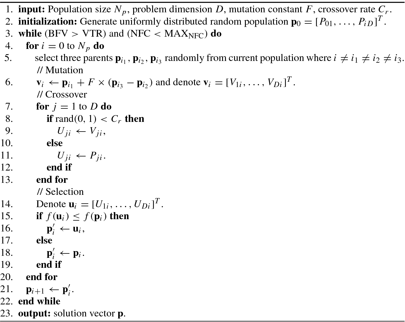
1. 1.
   Mutation: For each target vector , create the mutant individual by adding a weighted difference vector between two individuals and according to

   

   (9.11.2)

   where F > 0 is a constant coefficient used to control the differential variation . The evolution optimization based on difference vector between two populations or solutions is known as the differential evolution.

    
2. 2.
   Crossover: Denote . In order to increase the diversity of the perturbed parameter vectors, introduce crossover

   

   (9.11.3)

   for j = 1, 2, …, D, where rand_j(0, 1) is an uniformly distributed random number between 0 and 1, and j _rand is a randomly chosen index to ensure that the trial vector does not duplicate . CR ∈ (0, 1) is the crossover rate.

    
3. 3.
   Selection: To decide whether or not it should become a member of the next generation G + 1, the trial vector is compared to the target vector according to the fitness values of the parent individual and the trial individual , i.e.,

   

   (9.11.4)

   Here is the offspring of for the next generation.

    

9.11.2 Differential Evolution Variants

There are several schemes of DE based on different mutation strategies [124]:

(9.11.5)

(9.11.6)

(9.11.7)

(9.11.8)

(9.11.9)

where is the best vector in the population. , and are four different randomly selected vectors (where i ≠ r ₁ ≠ r ₂ ≠ r ₃ ≠ r ₄) from the current population.

These schemes can be unified by the notation DE∕a∕b∕c [101]. The meaning of a, b, c in this notation is as follows [101, 128].

• “a” specifies the vector which should be mutated; it can be the best vector (a = “best”) of the current population or a randomly selected one (a = “rand”).

• “b” denotes the number of difference vectors which participate in the mutation (b = 1 or b = 2).

• “c” denotes the applied crossover scheme, binary (c = “bin”) or exponential (c = “exp”).

The classical DE (9.11.5) with notation DE∕rand∕1∕bin and the scheme (9.11.7) with notation DE∕best∕2∕exp and exponential crossover are the most often used in practice due to their good performance [124, 166].

There are the following DE variants.

1. 1.
   Neighborhood search differential evolution (NSDE): it has been shown to play a crucial role in improving evolutionary programming (EP) algorithm’s performance [165]. The neighborhood search differential evolution (NSDE) developed in [162] is the same as the above classical DE except for mutation (9.11.2) replaced by

   

   (9.11.10)

   Here , N(0.5, 0.5) denotes a Gaussian random number with mean 0.5 and standard deviation 0.5, and δ denotes a Cauchy random variable with scale parameter 1.

    
2. 2.
   Self-adaptive differential evolution (SaDE): As compared with the classical DE of Storn and Price [147], the SaDE of Qin and Suganthan [125] has the following main differences: (a) SaDE adopts two different mutation strategies in single DE variant and introduces a probability p to control which mutation strategy to use, and p is gradually self-adapted according to the learning experience. (b) SaDE utilizes two methods to adapt and self-adapt DE’s parameters F and CR. The detailed operations of SaDE are summarized as follows:

   • Mutation strategies self-adaptation: SaDE selects mutation strategies (9.11.5) and (9.11.7) as candidates to create the mutant individual:

     

     (9.11.11)
     Here, the probability p is updated as

     

     (9.11.12)

     where ns1 and ns2 are, respectively, the number of offspring successfully entering the next generation while generated by Eqs. (9.11.5) and (9.11.7) after evaluation of all offspring; and both nf1 and nf2 are the numbers of offspring discarded while generated by Eqs. (9.11.5) and (9.11.7), respectively.

   • Scale factor F setting:

     

     (9.11.13)

     where N _i(0.5, 0.3) denotes a Gaussian random number with mean 0.5 and standard deviation 0.3.

   • Crossover rate CR self-adaptation: SaDE allocates a CR _i for each individuals:

     

     (9.11.14)
     with the updating formula

     

     (9.11.15)

     where CRm is set to 0.5 initially, and CRrec is the CR values associated with offspring successfully entering the next generation. CRrec will be reset once CRm is updated. This self-adaptation scheme for CR is denoted as SaCR.

    
3. 3.

   Self-adaptive NSDE (SaNSDE): This is an algorithm incorporating self-adaptive mechanisms into NSDE, see [166] for details.

    

On opposition-based differential evolution, an important extension to DE, we will present it in Sect. 9.15.

9.12 Ant Colony Optimization

In addition to evolutionary algorithms, another group of nature inspired metaheuristic algorithms is based on swarm intelligence in biology society.

Swarm intelligence refers to a kind of problem-solving ability through the interactions of simple information-processing units. Swarm intelligence includes two important concepts [85]:

1. 1.

   The concept of a swarm means multiplicity, stochasticity, randomness, and messiness.

    
2. 2.

   The concept of intelligence suggests that the problem-solving method is somehow successful.

    

The information-processing units that compose a swarm can be animate (such as ants, bees, fishes, etc.), mechanical, computational, or mathematical. Three famous swarm intelligence algorithms are ant colony algorithms, artificial bee colony algorithms, and swarm intelligence algorithms. In this section, we focus on ant colony algorithms.

The original inspired optimization idea behind ant algorithms came from observations of the foraging behavior of ants in the wild, and moreover, the phenomena called stigmergy [111]. By stigmergy, it means the indirect communication among a self-organizing emergent system via individuals modifying their local environment [59]. The stigmergic nature of ant colonies was explored by Deneubourg et al. in 1990 [27]: ants communicate indirectly by laying down pheromone trails, which ants then tend to follow.

Depending on the criteria being considered, modern heuristic algorithms for solving combinatorial and numeric optimization problems can be classified into the following four main different groups [82]:

• Population-based algorithm: An algorithm working with a set of solutions and trying to improve them is called population based algorithm.

• Iterative based algorithm: An algorithm using multiple iterations to approach the solution sought is named as iterative based algorithm.

• Stochastic algorithm: An algorithm employing a probabilistic rule for improving a solution is called probabilistic or stochastic algorithm.

• Deterministic algorithm: An algorithm employing a deterministic rule for improving a solution is known as deterministic algorithm.

The most popular population-based algorithm is evolutionary algorithms, and the most typical stochastic algorithms are swarm intelligence based algorithms. Both evolutionary algorithms and swarm intelligence based algorithms depend on the nature of phenomenon simulated by algorithms. As the most popular evolutionary algorithm, genetic algorithm attempts to simulate the phenomenon of natural evolution.

The two important swarm optimization algorithms are the ant colony optimization (ACO) algorithms and the artificial bee colony (ABC) algorithms. An ant colony can be thought of as a swarm whose individual agents are ants. Similarly, an artificial bee colony can be thought of as a swarm whose individual agents are bees.

Recently, ABC algorithm has been proposed to solve many difficult optimization problems in different fields such as constraint optimization problem, machine learning, and bioinformatics.

This section discusses ACO algorithms, and the next section discusses ABC algorithms.

9.12.1 Real Ants and Artificial Ants

In nature, the behavioral rules of ants are very simple, and their communication rules via “pheromones” are also very simple. However, a swarm of ants can solve very complex problems such as finding the shortest path between their nest and the food source. If finding the shortest path is looked upon as an optimization problem, then each path between the starting point (their nest) and the terminal (the food source) can be viewed as a feasible solution.

Each real ant in the ant system has the following characteristics [111]:

• By using a transition rule that is a function of the distance to the source, an ant decides which food source to go and the amount of pheromone present along the connecting path.

• Transitions to already visited food sources are added to a tabu list and are not allowed.

• Once a tour is complete, the ant lays a pheromone trail along each path visited in the source.

By Beckers, Deneubourg, and Goss [9], it was demonstrated experimentally that ants are able to find the shortest path.

Artificial ants of the colony have the following properties [21, 31]:

• An ant searches for minimum cost feasible solutions .

• An ant k has an internal memory which is used to store the path information followed by the ant k so far (i.e., the previously visited states). Memory can be used to build feasible solutions, to evaluate the solution found, and to retrace the path backward.

• An ant k in state S _r,i can move from node i to any node j in its feasible neighborhood .

• An ant k can be assigned a start state and one or more termination conditions e ^k. Usually, the start state is expressed as a unit length sequence, that is, a single component.

• Starting from an initial state S _initial, each ant tries to build a feasible solution to the given problem in an incremental way, moving to feasible neighbor states in an iterative fashion through its search space/environment. The construction procedure stops when for at least one ant k, at least one of the termination conditions e ^k is satisfied.

• The guidance factors involved in an ant’s movement take the form of a transition rule which is applied before every move from state S _i to state S _j. The transition rule may also include additional problem specific constraints and may utilize the ants internal memory.

• The ants’ probabilistic decision rule is a function of (a) the values stored in a node local data structure called ant-routing table, obtained by a functional composition of node locally available pheromone trails and heuristic values, (b) the ant’s private memory storing its past history, and (c) the problem constraints.

• When moving from node i to neighbor node j the ant can update the pheromone trail τ _ij on the arc (i, j). This is called online step-by-step pheromone update.

• Once built a solution, the ants can retrace their same path backward and update the pheromone trails on the traversed arcs. This is called online delayed pheromone update.

• The amount of pheromone each ant deposits is governed by a problem specific pheromone update rule.

• Ants may deposit pheromone associated with states, or alternatively, with state transitions.

• Once it has built a solution, and, if the case, after it has retraced the path back to the source node, the ant dies, freeing all the allocated resources.

Artificial ants have several characteristics similar to real ants, namely [122]:

1. (a)

   Artificial ants have a probabilistic preference for paths with a larger amount of pheromone.

    
2. (b)

   Shorter paths tend to have larger rates of growth in their amount of pheromone.

    
3. (c)

   Artificial ants use an indirect communication system based on the amount of pheromone deposited on each path.

    

By mimicking bionic swarm intelligence that simulates the behavior of ants and their communication ways in searching for food, ACO algorithms, as a heuristic positive feedback search algorithm, are especially available for solving the optimization problem including two parts: the feasible solution space and the objective function.

The key component of an ACO algorithm is a parameterized probabilistic model, which is called the pheromone model [30].

For a constrained combinatorial optimization problem, the central component of an ACO algorithm is also the pheromone model which is used to probabilistically sample the search space S.

Definition 9.37 (Pheromone Model [30])

A pheromone model P = (S,  Ω, f) of a combinatorial optimization problem consists of two parts:

1. (1)

   a search (or solution) space S defined over a finite set of discrete decision variables and a set Ω of constraints among the variables and

    
2. (2)

   an objective function to be minimized, which assigns a positive cost function to each solution s ∈ S.

    

The problem representation of a combinatorial optimization problem which is exploited by the ants can be characterized as follows [33].

• A finite set of components is given.

• The states of the problem are defined in terms of sequences x = {c _i, c _j, …, c _k, …} over the elements of C. The set of all possible sequences is denoted by X. The length of a sequence x, that is, the number of components in the sequence, is expressed by |x|. The maximum length of a sequence is bounded by a positive constant n < +∞.

• The set of (candidate) solutions S is a subset of X (i.e., S ⊆ X).

• The finite set of constraints Ω defines the set of feasible states with .

• A non-empty set S ^∗ of feasible solutions is given, with and S ^∗⊆ S.

• A cost f(s, t) is associated with each candidate solution s ∈ S.

• In some cases a cost, or the estimate of a cost, J(x _i, t), can be associated with states other than solutions. If x _i can be obtained by adding solution components to a state x _j, then J(x _i, t) ≤ J(x _j, t). Note that J(s, t) ≡ J(t, s).

In combinatorial optimization a system may occur in many different configurations. Any configuration has a cost function for that particular configuration. Similar to the simulated annealing of solids, one can statistically model the evolution of the system to be optimized into a state that corresponds with the minimum cost function value.

In order to probabilistically construct solutions, ACO algorithms for combinatorial optimization problems use a pheromone model that consists of a set of pheromone values, i.e., a function of the search experience of the algorithm. The pheromone model is used to bias the solution construction toward regions of the search space containing high-quality solutions.

Definition 9.38 (Mixed-Variable Optimization Problem [95])

A pheromone model R = (S,  Ω, f) of a mixed-variable optimization problem (MVOP) consists of the following parts.

• A search space S defined over a finite set of both discrete and continuous decision variables and a set Ω of constraints among the variables;

• An objective function to be minimized. The search space S is defined by a set of n = d + r variables x _i, i = 1, …, n, of which d is the number of discrete decision variables and r is the number of continuous decision variables. A solution s ∈ S is a complete value assignment, that is, each decision variable is assigned a value. A feasible solution is a solution that satisfies all constraints in the set Ω. A global optimum s ^∗∈ S is a feasible solution satisfying f(s ^∗) ≤ f(s), ∀s ∈ S. The set of all globally optimal solutions is denoted by s ^∗∈ S ^∗⊆ S. Solving an MVOP requires finding at least one s ^∗∈ S ^∗.

9.12.2 Typical Ant Colony Optimization Problems

Ant colony optimization is so called because of its original inspiration: some ant species forage between their nests and food sources by collectively exploiting the pheromone they deposit on the ground while walking [29]. Similar to real ants, artificial ants in ant colony optimization deposit artificial pheromone on the graph of the problem they are solving.

In ant colony optimization, each individual of the population is an artificial ant that builds incrementally and stochastically a solution to the considered problem. At each step the moves of ants define which solution components are added to the solution under construction.

A probabilistic model is associated with the graph G(C, L) and is used to bias the agents’ choices. The probabilistic model is updated online by the agents in order to increase the probability that future agents will build good solutions.

In order to build good solutions, there are three main construction functions (ACO construction functions for short) [111]:

• Ant solution construct: In the solution construction process, artificial ants move through adjacent states of a problem according to a transition rule, iteratively building solutions.

• Pheromone update: It performs pheromone trail updates and may involve updating the pheromone trails once complete solutions have been built, or updating after each iteration.

• Deamon actions: It is an optional step in the ant colony optimization and involves applying additional updates from a global perspective (there exists no natural counterpart). An example could be applying additional pheromone reinforcement to the best solution generated (known as offline pheromone trail update).

The following are the three typical optimization problems whose solutions are available for adopting ant colony optimization.

1. 1.
   Job Scheduling Problems (JSP) [105] have a vital role in recent years due to the growing consumer demand for variety, reduced product life cycles, changing markets with global competition, and rapid development of new technologies. The job shop scheduling problem (JSSP) is one of the most popular scheduling models existing in practice, which is among the hardest combinatorial optimization problems. The job scheduling problem consists of the following components:

   • a number of independent (user/application) jobs to be the elements in C,

   • a number of heterogeneous machine candidates to participate in the planning,

   • the workload of each job (in millions of instructions),

   • the computing capacity of each machine,

   • ready time indicates when machine will have finished the previously assigned jobs, and

   • the expected time to compute (ETC) matrix (“n _b” jobs × “n _b” numbers of components machines) in which ETC[i][j] is the expected execution time of job “i” in machine “j.”

    
2. 2.
   Data mining [122]: In an ant colony optimization algorithm, each ant incrementally constructs/modifies a solution for the target problem.

   • In the context of classification task of data mining, the target problem is the discovery of classification rules that is often expressed in the form of IF-THEN rules as follows:

     

     The rule antecedent (IF part) contains a set of conditions, usually connected by a logical conjunction operator (AND). The rule consequent (THEN part) specifies the class predicted for cases whose predictor attributes satisfy all the terms specified in the rule antecedent. As a promising research area, ACO algorithms involve simple agents (ants) that cooperate with others to achieve an emergent unified behavior for the system as a whole, producing a robust system capable of finding high-quality solutions for problems with a large search space.

   • In the context of rule discovery, an ACO algorithm is able to perform a flexible robust search for a good combination of terms (logical conditions) involving values of the predictor attributes.

    
3. 3.

   Network coding resource minimization (NCRM) problem [156]: As a resource optimization problem emerging from the field of network coding, although all nodes have the potential to perform coding would perform coding by default, only a subset of coding-possible nodes suffices to realize network coding-based multicast (NCM) with an expected data rate. Hence, it is worthwhile to study the problem of minimizing coding operations within NCM. EAs are the mainstream solutions for NCRM in the field of computational intelligence, but EAs are not good for integrating local information of the search space or domain-knowledge of the problem, which could seriously deteriorate their optimization performance. Different from EAs, ACO algorithms are the classes of reactive search optimization methods adopting the principle of “learning while optimizing.” ACOs may be a good candidate for solving the NCRM problem.

    

9.12.3 Ant System and Ant Colony System

As the first ant algorithm, ant system was developed by Dorigo et al. in 1996 [34] for applying the well-known benchmark traveling salesman problem.

Let τ _ij be the pheromone trail between components (nodes) i and j that determines the path taken by the ants, and η _ij = 1∕d _ij be the heuristic values, where τ _ij constitute the pheromone matrix T = [τ _ij]. In other words, the shorter the distance d _ij between two cities i and j, the higher the heuristic value η _ij that constitutes the heuristic matrix.

The values from multiple pheromone (or heuristic) matrices need to be aggregated into a single pheromone (or heuristic) value. The following are the three alternatives of aggregation [97]:

1. 1.
   Weighted sum: for example

   

   (9.12.1)
    
2. 2.
   Weighted product: for example

   

   (9.12.2)
    
3. 3.

   Random: at each construction step, given a uniform random number U(0, 1), an ant selects the first of the two matrices if U(0, 1) < 1 − λ; otherwise, it selects the other matrix.

    

The ants exists in an environment represented mathematically as a construction graph G(C, L).

1. 1.

   denotes a set of components, where c _i is the ith city and N _c is the number of all cities in tour.

    
2. 2.

   L is a set of connections fully connecting.

    

By Dorigo et al. [34] and Neto and Filho [115], ant model has the following characteristics:

• The ant always occupies a node in a graph which represents a search space. This node is called nf.

• It has an initial state.

• Although it cannot sense the whole graph, it can collect two kinds of information about the neighborhood: (a) the weight of each trail linked to nf and (b) the characteristics of each pheromone deposited on this trail by other ants of the same colony.

• It moves toward a trail C _ij that connects nodes i and j of the graph.

• Also, it can alter the pheromones of the trail C _ij, in an operation called as “deposit of pheromone levels.”

• It can sense the pheromone levels of all C _ij trails that connect a node i.

• It can determine a set of “prohibited” trails.

• It presents a pseudo-random behavior enabling the choice among the various possible trails.

• This choice can be (and usually is) influenced by the level of pheromone.

• It can move from node i to node j.

An ant system utilizes the graph representation G(C, L): for each cost measure δ(r, s) (distance from city r moving to city s), each edge (r, s) has also a desirability measure (called pheromone) τ _rs = τ(r, s) which is updated at run time by ants.

An ant system works according to the following rules [32]:

1. 1.

   State transition rule: Each ant generates a complete tour by choosing the cities according to a probabilistic state transition rule; ants prefer to move to cities which are connected by short edges with a high amount of pheromone.

    
2. 2.

   Global (pheromone) updating rule: Once all ants have completed their tours, a global updating rule is used; a fraction of the pheromone evaporates on all edges, and then each ant deposits an amount of pheromone on edges which belong to its tour in proportion to how short its tour was. The process is then iterated.

    
3. 3.
   Random-proportional rule: It gives the probability with which the kth ant in city r chooses to move to the city s:

   

   (9.12.3)

   Here τ is the pheromone, η = 1∕δ is the inverse of the distance δ(r, s), J _k(r, s) is the set of cities that remain to be visited by ant k positioned on city r (to make the solution feasible), and β > 0 is a parameter for determining the relative importance of pheromone versus distance.

    

In the way given by (9.12.3), the ants favor the choice of edges which are shorter and have a greater amount of pheromone.

In an ant system, once all ants have built their tours, pheromone is updated on all edges according to the following global updating rule:

(9.12.4)

where

(9.12.5)

Here 0 < α < 1 is a pheromone decay parameter, L _k is the length of the tour performed by ant k, and m is the number of ants.

The ant colony system (ACS) differs from the ant system in three main aspects [32]:

• State transition rule provides a direct way to balance between exploration of new edges and exploitation of a priori and accumulated knowledge about the problem.

• Global updating rule is applied only to edges which belong to the best ant tour.

• A local (pheromone) updating rule is applied while ants construct a solution.

Different from ant system, ant colony system works according to the following rules [32]:

1. 1.
   ACS state transition rule: In ACS, an ant positioned on node r chooses the city s to move to by applying the ACS state transition rule given by

   

   (9.12.6)

   Here q is a random number uniformly distributed in [0, 1], 0 ≤ q ₀ ≤ 1 is a parameter, and S is a random variable selected according to the probability distribution given in (9.12.3). The state transition rule given by (9.12.6) and (9.12.3) is known as pseudo-random-proportional rule. This rule favors transitions toward nodes connected by short edges and with a large amount of pheromone.

    
2. 2.
   ACS global updating rule: In ACS only the globally best ant, constructed the shortest tour from the beginning of the trial, is allowed to deposit pheromone. After all ants have completed their tours, the pheromone level is updated by the following ACS global updating rule:

   

   (9.12.7)

   where

   

   (9.12.8)

   Here 0 < α < 1 is the pheromone decay parameter, and L _gb is the length of the globally best tour from the beginning of the trial.

    
3. 3.
   ACS local updating rule: While building a solution (i.e., a tour) of the traveling salesman problem (TSP), ants visit edges and change their pheromone level by applying the following local updating rule:

   

   (9.12.9)

   where 0 < ρ < 1 is a parameter.

    

9.13 Multiobjective Artificial Bee Colony Algorithms

Artificial bee colony (ABC) algorithm, proposed by Karaboga in 2005 [81], is inspired by the intelligent foraging behavior of the honey bee swarm. Numerical comparisons show that the performance of ABC is competitive to that of other population-based algorithms with an advantage of employing fewer control parameters [82–84]. The main advantages of ABC are its simplicity and ease of implementation, but ABC also faces up to the poor convergence commonly existing in evolutionary algorithms.

9.13.1 Artificial Bee Colony Algorithms

The design of an ant colony optimization (ACO) algorithm implies the specification of the following aspects [11, 99, 122]:

• An appropriate representation of the problem, which allows the ants to incrementally construct/modify solutions through the use of a probabilistic transition rule, based on the amount of pheromone in the trail and on a local problem-dependent heuristic.

• A method to enforce the construction of valid solutions, i.e., solutions that are legal in the real-world situation corresponding to the problem definition.

• A problem dependent heuristic function η that provides a quality measurement of items that can be added to the current partial solution.

• A rule for pheromone updating, which specifies how to modify the pheromone trail τ.

• A probabilistic transition rule based on the value of the heuristic function η and on the contents of the pheromone trail τ that is used to iteratively construct a solution.

• A clear specification of when the algorithm converges to a solution.

Unlike ant swarms, the collective intelligence of honey bee swarms consists of three essential components: food sources, employed bees, unemployed (onlooker) bees.

In the ABC algorithm, the position of a food source represents a possible solution of the optimization problem and the nectar amount of a food source corresponds to the quality (fitness) of the associated solution. The artificial bee colony is divided into three groups of bees: employed bees, onlooker bees, and scout bees. Half of the colony consists of the employed bees, and another half consists of the onlookers.

Each cycle of the search consists of three steps.

• Employed bees are responsible for exploring the nectar sources and sharing their food information with onlookers within the hive.

• The onlooker bees select good food sources from those foods found by the employed bees to further search the foods.

• If the quality of some food source is not improved through a predetermined number of cycles, then the food source is abandoned by its employed bee, and the employed bee becomes a scout and starts to search for a new food source randomly in the vicinity of the hive.

Each food source x _i = [x _i,1, …, x _i,D]^T (i = 1, …, SN) is a D-dimensional vector, and stands for a potential solution of the problem to be optimized. Let P = {x ₁, …, x _SN} denotes the population of SN food solutions (individuals). The ABC algorithm is an iterative algorithm. At the beginning, ABC generates the population with randomly generated food solutions. The newly generated population P contains SN individuals , where the population size SN is identical to the number of those different kinds of bees. ABC generates a randomly distributed initial population P of SN solutions (food source positions) x ₁, …, x _SN whose elements are as follows:

(9.13.1)

where i = 1, …, SN; j = 1, …, D, and D is the number of optimization parameters; and are the lower and upper bounds for the dimension j, respectively; and U(0, 1) is a random number with uniform distribution in (0, 1).

After the initialization, the population of solutions (i.e., food sources) undergoes repeated cycles of the search processes of the employed bees, onlooker bees, and scout bees. Each employed bee always remembers its previous best position and produces a new position within its neighborhood in its memory.

After all employed bees finish their search process, they will share the information about nectar amounts and positions of food sources with onlookers. Each onlooker chooses a food source depending on the probability value p _i associated with the food source through

(9.13.2)

where fit_i represents the fitness value of the ith solution f(x _i).

If the new food source has the equal or better quality than the old source, then the old source is replaced by the new source. Otherwise, the old source is retained. ABC uses

(9.13.3)

to produce a candidate food position from the old solution x _i in memory. Here, l ∈{1, …, SN} and j ∈{1, …, D} are randomly chosen indices, and ϕ _ij is a random number in the range [−1, 1].

Then, ABC searches the area within its neighborhood to generate a new candidate solution. If a position cannot be improved further through a predetermined number of cycles, then that food source is said to be abandoned. The value of the predetermined number of cycles is an important control parameter of ABC, and is called the limit for abandonment. When the nectar of a food source is abandoned, the corresponding employed bee becomes a scout. The scout will randomly generate a new food source to replace the abandoned position.

The above framework of artificial bee colony (ABC) algorithm is summarized as Algorithm 9.15.

Algorithm 9.15 Framework of artificial bee colony (ABC) algorithm [49]

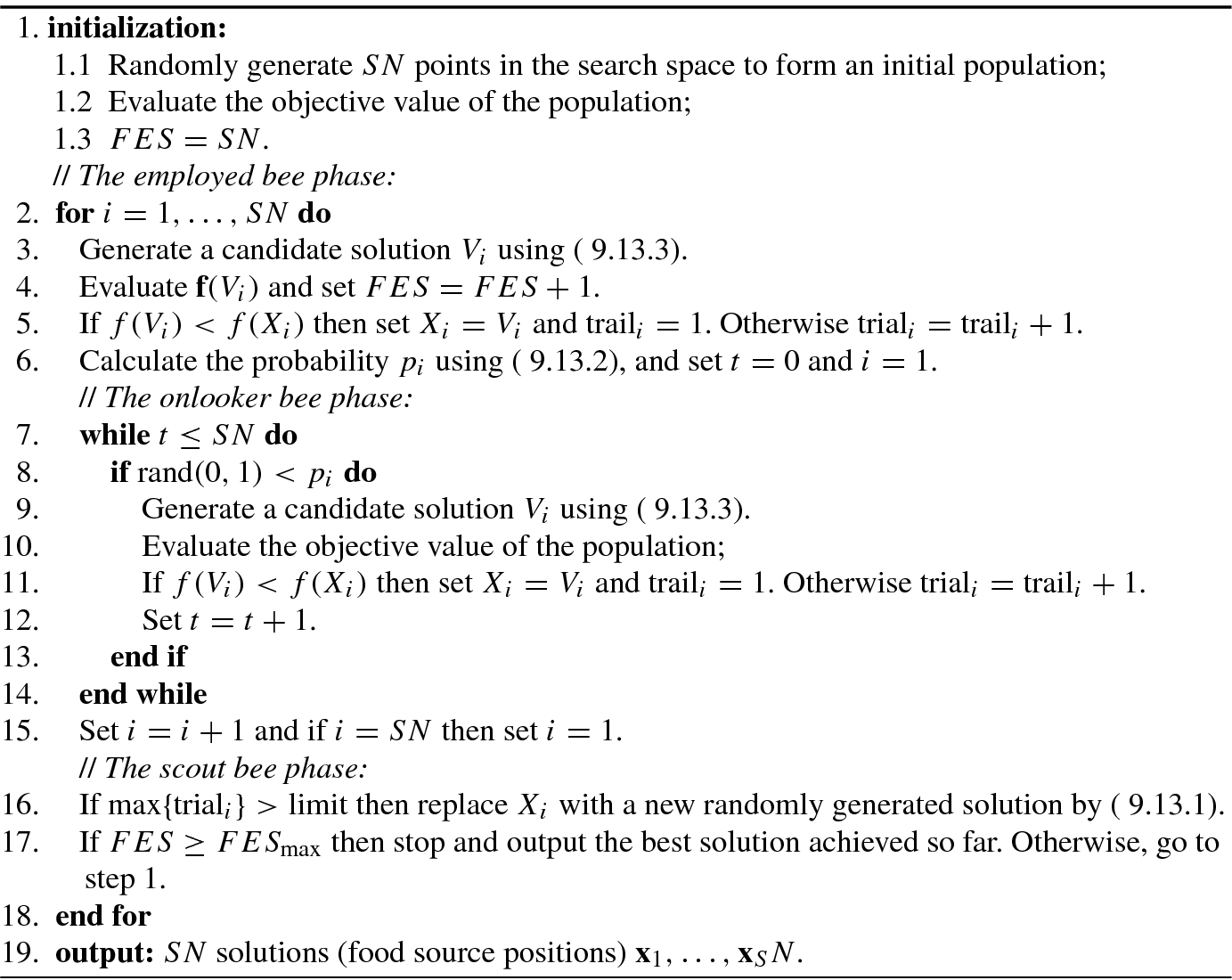
9.13.2 Variants of ABC Algorithms

The solution search equation of ABC, for generating new candidate solutions based on the information of previous solutions, is good at exploration, but it is poor at exploitation. To achieve good performance on problem optimizations, exploration and exploitation should be well balanced.

To improve the performance of ABC, several variants of ABC were proposed.

1. 1.
   GABC: This a gbest-guided artificial bee colony algorithm [168]. By incorporating the information of the gbest solution into the solution search equation to improve the exploitation of ABC. The solution search equation in GABC is given by

   

   (9.13.4)

   where the third term in the right-hand side is a new added term called the gbest term, g _j is the jth element of the gbest solution vector , ϕ _ij is a random number in the range [−1, 1], and ψ _ij is a uniform random number in [0, 1.5]. As demonstrated by experimental results, GABC can outperform ABC in most experiments.

    
2. 2.
   IABC: This is an improved artificial bee colony (IABC) algorithm [48]. In this algorithm, two improved solution search equations are given by

   

   (9.13.5)

   

   (9.13.6)

   where the indices r1 and r2 are mutually exclusive integers randomly chosen from {1, 2, …, SN}, and both of them are different from the base index i; g _best,j is the jth element of the best individual vector with the best fitness in the current population, and j ∈{1, …, D} is a randomly chosen index. Since (9.13.5) generates a candidate solution around g _best, it focuses on the exploitation. On the other hand, as (9.13.6) is based on three vectors x _i, x _r1, and x _r2, and the two latter ones are two different individuals randomly selected from the population, it emphasizes the exploration.

    
3. 3.
   CABC: The solution search equation is given by Gao et al. [49]

   

   (9.13.7)

   where the indices r1 and r2 are distinct integers uniformly chosen from the range [1, SN] and are also different from i, and ϕ _ij is a random number in the range [−1, 1]. Since (9.13.7) looks like the crossover operator of GA, the ABC with this search equation is named as crossover-like artificial bee colony (CABC) [49].

    

9.14 Particle Swarm Optimization

Particle swarm optimization (PSO) is a global optimization technique originally developed by Eberhart and Kennedy [36, 86] in 1995. PSO is essentially an optimization technique based on swarm intelligence, and adopts a population-based stochastic algorithm for finding optimal regions of complex search spaces through the interaction of individuals in a population of particles. Different from evolutionary algorithms, the particle swarm does not use selection operation; while interactions of all population members result in iterative improvement of the quality of problem solutions from the beginning of a trial until the end.

PSO is rooted in artificial life and social psychology, as well as in engineering and computer science. It is widely recognized (see, e.g., [19, 37, 85]) that swarm intelligence (SI) is an innovative distributed intelligent paradigm for solving optimization problems, and PSO was originally inspired by the swarming behavior observed in flocks of birds, swarms of bees, or schools of fish, and even human social behavior, from which the idea is emerged.

Due to computational intelligence, PSO is not largely affected by the size and nonlinearity of the optimization problem, and can converge to the optimal solution in many problems where most analytical methods fail to converge.

In PSO, the term “particles” refers to population members with an arbitrarily small mass or volume and is subject to velocities and accelerations towards a better mode of behavior.

9.14.1 Basic Concepts

PSO is based on two fundamental disciplines: social science and computer science, and is closely based on the swarm intelligence concepts and principles [26].

1. 1.

   Social concepts: It is known [37] that “human intelligence results from social interaction.” Evaluation, comparison, and imitation of others, as well as learning from experience allow humans to adapt to the environment and determine optimal patterns of behavior, attitudes, and so on.

    
2. 2.
   Swarm intelligence principles [ 37, 85, 86]: Swarm Intelligence can be described by considering the following five fundamental principles.

   • Proximity principle: the population should be able to carry out simple space and time computations.

   • Quality principle: the population should be able to respond to quality factors in the environment.

   • Diverse response principle: the population should not commit its activity along excessively narrow channels.

   • Stability principle: the population should not change its mode of behavior whenever the environment changes.

   • Adaptability principle: the population should be able to change its behavior mode when it is worth the computational price.

    
3. 3.
   Computational characteristics [ 37]: As a useful paradigm for implementing adaptive systems, the swarm intelligence computation is an extension of evolutionary computation and includes the softening parameterization of logical operators like AND, OR, and NOT. In particular, PSO is an extension, and a potentially important incarnation of cellular automata (CA). The particle swarm can be conceptualized as cells in CA, whose states change in many dimensions simultaneously. Both PSO and CA share the following computational attributes.

   • Individual particles (cells) are updated in parallel.

   • Each new value depends only on the previous value of the particle (cell) and its neighbors.

   • All updates are performed according to the same rules.

    

9.14.2 The Canonical Particle Swarm

Given an unleveled data set Z = {z ₁, …, z _N} representing N patterns , each having D features. Then partitional clustering approach aims at clustering the data set into K groups (K ≤ N) such that

(9.14.1)

(9.14.2)

The clustering operation is dependent on the similarity between elements present in the data set. If f denotes the fitness function, then the clustering task can be viewed as an optimization problem: . That is to say, the optimization based clustering task is carried out by single objective nature inspired metaheuristic algorithms.

PSO is inspired by social interaction (e.g., foraging process of bird flocking). The original concept of PSO is to simulate the behavior of flying birds and their means of information exchange to solve problems. In PSO, each single solution is like a “bird.” Imagine the following scenario: a group of birds are randomly searching food in an area in which only one piece of food is assumed to exist, and the birds do not know where the food is. An efficient strategy for finding the food is to follow the bird nearest to the food.

In a particle swarm optimizer, instead of using genetic operators, each single solution is regarded as a “bird” (particle or individual) in the search space. These individuals are “evolved” by cooperation and competition among the individuals themselves through generations. Each particle adjusts its flying according to its own flying experience and its companions’ flying experience. Each individual or particle represents a potential solution to an optimization problem, and is treated as a point in a D-dimensional space.

Define the notations and parameters as follows.

• N _p: the swarm (or population) size;

• x _i(t): the position vector of the ith particle at time t in the search space;

• v _i(t): the velocity vector of the ith particle at time t in the search space;

• : the previous best position (the position giving the best fitness value, simply named pbest) of the ith particle (up to time t) in the search space;

• : the best particle found so far among all the particles in the population, and is named as the global best position (gbest) vector of the swarm;

• U(0, β): a uniform random number generator;

• α: inertia weight or constriction coefficient;

• β: acceleration constant.

Position and velocity of each particle are adjusted, and the fitness function with the new position is evaluated at each time step. A population of particles at the time t is initialized with random position of the ith particle at the time t, , and the velocity of the ith particle at the time t, .

The most common type of implementation defines the particles’ behaviors in the following two formulas [19, 85]. First adjust the step size of the particle:

(9.14.3)

and then move the particle by adding the velocity to its previous position:

(9.14.4)

By Clerc and Kennedy [19], though there is variety in the implementations of the particle swarm, the most standard version uses α = 0.7298 and β = ψ∕2, where ψ = 2.9922.

The personal best position of each particle is updated using

(9.14.5)

for i = 1, …, N _p, and the global best position g _best found by any particle during all previous steps is defined as

(9.14.6)

The basic particle swarm optimization algorithm is shown in Algorithm 9.16.

Algorithm 9.16 Particle swarm optimization (PSO) algorithm

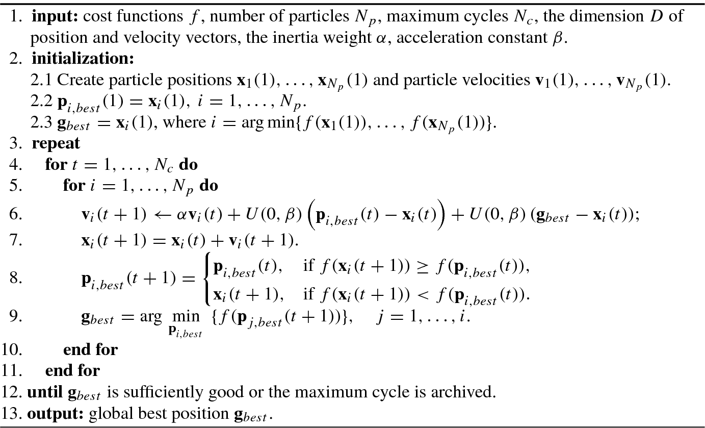
9.14.3 Genetic Learning Particle Swarm Optimization

Advantages of PSO over other similar optimization techniques such as GA can be summarized as follows [26]:

• PSO is easier to implement and there are fewer parameters to adjust.

• In PSO, every particle remembers its own previous best value as well as the neighborhood best; therefore, it has a more effective memory capability than the GA.

• PSO is more efficient in maintaining the diversity of the swarm [38] (more similar to the ideal social interaction in a community), since all the particles use the information related to the most successful particle in order to improve themselves, whereas in GA, the worse solutions are discarded and only the good ones are saved; therefore, in GA the population evolves around a subset of the best individuals.

The following are the two main drawbacks of PSO [123].

1. 1.
   The swarm may prematurely converge.

   • For the global best PSO, particles converge to a single point, which is on the line between the global best and the personal best positions. This point is not guaranteed for a local optimum [154].

   • The fast rate of information flow between particles, resulting in the creation of similar particles with a loss in diversity that increases the possibility of being trapped in local optima.

    
2. 2.

   Stochastic approaches have problem-dependent performance. This dependency usually results from the parameter settings in each algorithm. Increasing the inertia weight will increase the speed of the particles resulting in more exploration (global search) and less exploitation (local search) will decrease the speed of the particles resulting in more exploitation and less exploration.

    

The problem-dependent performance can be addressed via hybrid mechanism combining different approaches in order to be benefited from the advantages of each approach. The following are the comparison between PSO and GA.

• In general PSO, particles are guided by their previous best positions (pbests) and the global best position (gbest) found by the swarm, so the search is more directional than that of GA. Hence, it is expected that GA possesses a better exploration ability than PSO, whereas the latter facilitates faster convergence.

• By applying crossover operation in GA, information can be swapped between two particles to have the ability to fly to the new search area. If applying mutation used in GA to PSO, then it is expected to increase the diversity of the population and the ability to have the PSO to avoid the local maxima.

This hybrid of genetic algorithm and particle swarm optimization is simply called GA-PSO, which combines the advantages of swarm intelligence and a natural selection mechanism in GA, and thus increases the number of highly evaluated agents, while decreases the number of lowly evaluated agents at each iteration step.

An alternative of GA-PSO is the genetic learning particle swarm optimization (GL-PSO) in [57], as shown in Algorithm 9.17.

Algorithm 9.17 Genetic learning PSO (GL-PSO) algorithm [57]

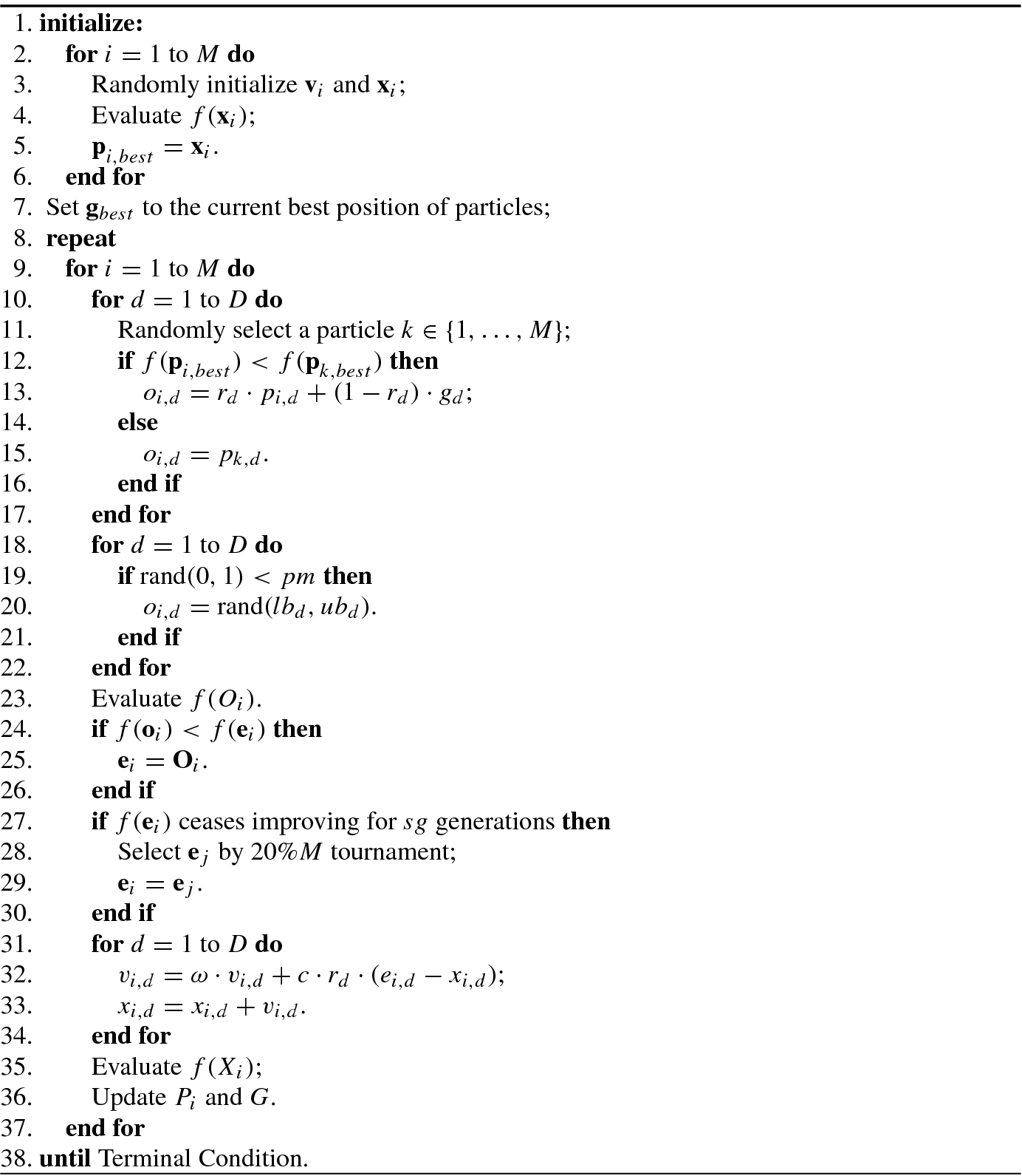
The GL-PSO is an optimization algorithm hybridized by genetic learning and particle swarm optimization hybridized in a highly cohesive way.

9.14.4 Particle Swarm Optimization for Feature Selection

To find the optimal feature subset one needs to enumerate and evaluate all the possible subsets of features in the entire search space, which implies that the search space size is 2ⁿ where n is the number of the original features. Therefore, evaluating the entire feature subset is computationally expensive and also impractical even for a moderate-sized feature set.

Although many feature selection algorithms involve heuristic or random search strategies to find the optimal or near optimal subset of features in order to reduce the computational time, metaheuristic algorithms may clearly be more efficient for feature subset selection.

Consider feature selection in supervised classification. Given the data set S = {(x ₁, y ₁), …, (x _n, y _n)}, where x _i = [x _i1, …, x _id]^T is a multi-dimensional vector sample, d denotes the number of features, n is the number of samples, and y _i ∈ I = {1, …, d} denotes the label of the sample x _i. Let X = {x ₁, …, x _n}. The main goal of the supervised learning is to approximate a function f : X → I to predict the class label for a new input vector x.

In the learning problems, choice of the optimization method is very important to reduce the dimensionality of the feature space and to improve the convergence speed of the learning model. The PSO method would be preferred because it can handle a large number of features.

Potential advantages of PSO for feature selection can be summarized as follows [138]:

• PSO has a powerful exploration ability until the optimal solution is found because different particles can explore different parts of the solution space.

• PSO is particularly attractive for feature selection since the particle swarm has memory, and knowledge of the solution is retained by all particles as they fly within the problem space.

• The attractiveness of PSO is also due to its computationally inexpensive implementation that still gives decent performance.

• PSO works with the population of potential solutions rather than with a single solution.

• PSO can address binary and discrete data.

• PSO has better performance compared to other feature selection techniques in terms of memory and runtime and does not need complex mathematical operators.

• PSO is easy to implement with few parameters, and is easy to realize and gives promising results.

• The performance of PSO is almost unaffected by the dimension of the problem.

Although PSO provides a global search strategy for finding a better solution in the feature selection task, it is infected with two shortcomings: premature convergence and weakness in fine-tuning near local optimum points. To overcome these weaknesses, a hybrid feature selection method based on PSO with local search, called HPSO-LS, was developed in [106].

Define the relevant symbols are as follows. n _f denotes the number of the original features in a given data set, n _s = |X _s| is the number of the selected features, c _ij is the Pearson correlation coefficient between two features x _i and x _j, cor_i is the correlation value for feature i, is the best previously visited position (up to time t) of the ith particle, is the global best position of the swarm, is the position of the dth dimension of the ith particle, v _i(t) is the velocity of the ith particle, x _i(k) and x _j(k) denote the values of the feature vectors i and j for the kth sample.

The pseudo code of the HPSO-LS algorithm is shown in Algorithm 9.18.

Algorithm 9.18 Hybrid particle swarm optimization with local search (HPSO-LS) [106]

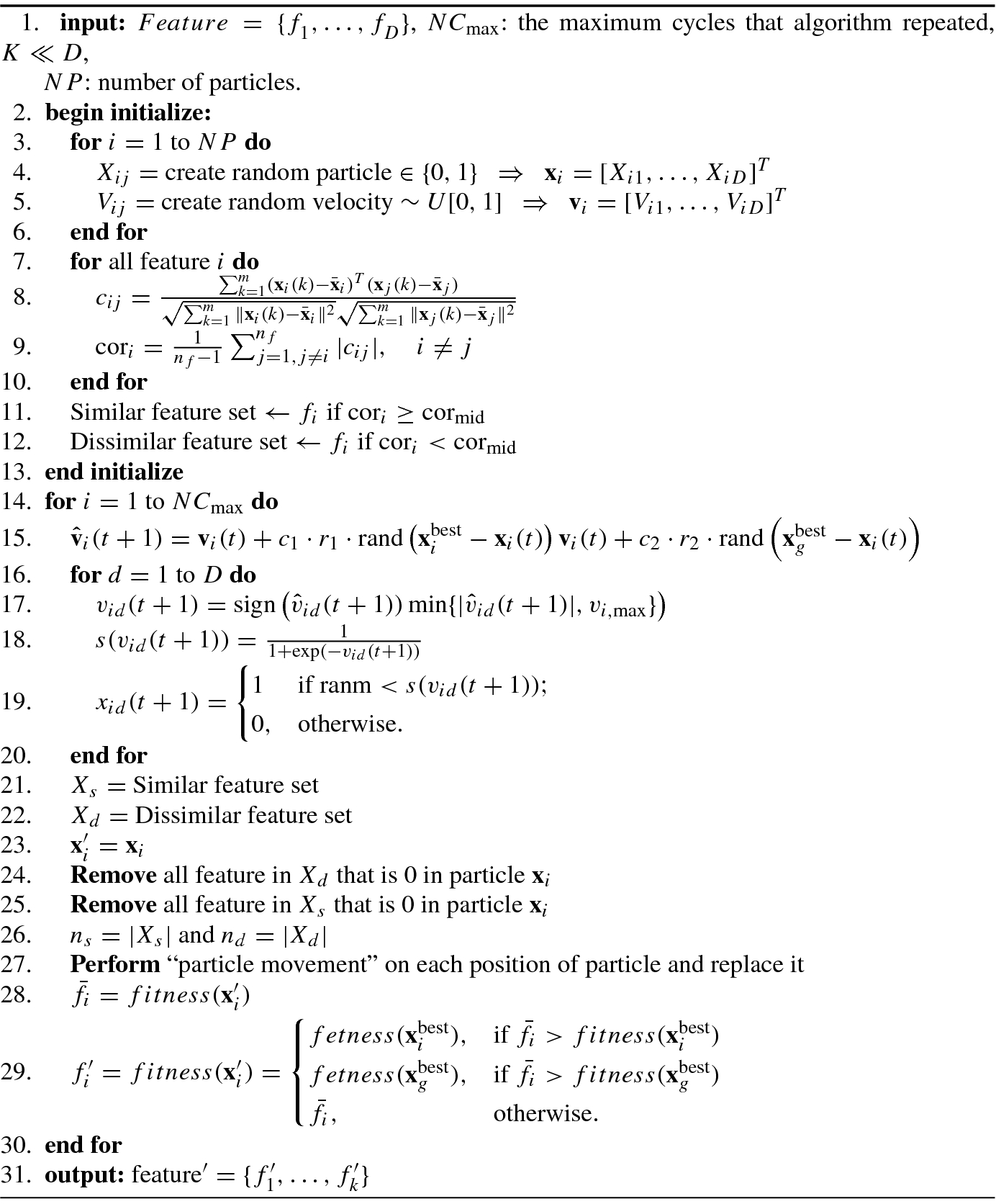
9.15 Opposition-Based Evolutionary Computation

It is widely recognized that hybridization with different algorithms is another direction for improving machine intelligence algorithms.

Learning, search, and optimization are fundamental tasks in the machine intelligence: Artificial intelligence algorithms learn from past data or instructions, optimize estimated solutions, and search for an existing solution in large spaces. In many cases, the machine learning starts at a random point, such as weights of a neural network, initial population of soft computing algorithms, and action policy of reinforcement agents. If the starting point is close to the optimal solution, then its convergence is faster. On the other hand, if it is very far from the optimal solution, such as opposite location in the worst case, the convergence will take much more time or even the solution can be intractable. In these bad cases, looking simultaneously for a better candidate solution in both current and opposite directions may help us to solve the present problem quickly and efficiently, which could be beneficial.

Opposition-based evolutionary computation is inspired in part by the observation that opposites permeate everything around us, in some form or another.

9.15.1 Opposition-Based Learning

There are several definitions on opposition of an existing solution x. Focused on metaheuristics and optimization, opposition is presented as a relationship between a pair of candidate solutions. In combinatorial and continuous optimization, each candidate solution has its own particularly defined opposite candidate.

Definition 9.39 (Opposite Number [151])

Let be a real number defined on a certain interval: x ∈ [a, b]. The opposite number x̆ is defined as

(9.15.1)

The opposite number in a multidimensional case can be analogously defined.

Figure 9.4 shows opposite number of a real number x.

Fig. 9.4

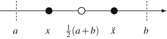
Geometric representation of opposite number of a real number x

Definition 9.40 (Opposite Point [131, 151])

Let be a point (vector) in D-dimensional space, where and . The opposite point is completely defined by its components

(9.15.2)

Theorem 9.9 (Uniqueness [130])

Every point of real numbers with x _i ∈ [a _i, b _i] has a unique opposite point defined by .

Definition 9.41 (Opposite Solution)

Given a candidate solution in a d-dimensional vector space, its opposition solution is defined as element form:

(9.15.3)

and generalized opposition solution is defined as

(9.15.4)

where k a random number in [0, 1]; while a _i and b _i are the minimum and maximum values for ith element of x.

Center-based sampling (CBS) [129] is a variant of opposition solution similar to generalized opposition solution.

Definition 9.42 (Center-Based Sampling [129, 135])

Let be a solution in a D-dimension vector space. An opposite candidate solution is defined by a random point between x and its opposite point as follows:

(9.15.5)

where rand_i is a uniformly distributed random number in [0, 1]; and a _i and b _i are the minimum and maximum values of the ith component of x.

The objective of center-based sampling is to obtain opposite candidate solutions closer to the center of the domain of each variable.

Definition 9.43 (Opposition-Based Learning [151])

Let and be a solution point and its opposition solution point in D-dimensional vector space, respectively. If the opposition solution has the better fitness, i.e., , then the original solution x should be replaced with the new candidate solution ; otherwise, x is continue to be used as a candidate solution. This machine learning based on opposition is called opposition-based learning (OBL). The optimization using the candidate solution and its opposition solution simultaneously for searching the better one is referred to as the opposition-based optimization (OBO).

The basic concept of OBL was originally introduced by Tizhoosh in 2005 [151]. The OBL has been applied in evolutionary algorithms, differential evolution, particle swarm optimization, harmony search, among others (see, e.g., Survey Papers [135, 161]).

9.15.2 Opposition-Based Differential Evolution

For evolutionary optimization methods, they start with some initial solutions (initial population) and try to improve them toward some optimal solution(s). In the absence of a priori information about the solution, some initial solutions are needed to be randomly guessed. Then, evolutionary optimization is related to the distance of these initial guesses from the optimal solution. An important fact is [131] that evolutionary optimization can be improved, if it starts with a closer (fitter) solution by simultaneously checking the opposite solution.

Let be a candidate solution in D-dimensional space, and be the opposite solution in D-dimensional space. Assume that f(p) is a fitness function for point p, which is used to measure the candidate’s fitness. If f(p̆) ≥ f(p), then point p can be replaced with p̆; otherwise, continue with p. Hence, the point p and its opposite point p̆ are evaluated simultaneously in order to continue with the fitter one.

By applying the OBL to the classical DE, Rahnamayan et al. [131] developed an opposition-based differential evolution (ODE).

The ODE consists of the following two OBL parts [131].

1. 1.
   Opposition-based population initialization:

   • Initialize the population randomly, here p _i = [P_i1, …, P_iD]^T.

   • Calculate opposite population by OP_ij = a _j + b _j −P_ij for i = 1, …, N _p; j = 1, …, D. Here, P_ij and OP_ij denote jth variable of the ith vector of the population and the opposite-population, respectively.

   • Select the N _p fittest individuals from {P ∪OP} as initial population.

    
2. 2.

   Opposition-based generation jumping: This part forces the evolutionary process to jump to a new solution candidate which ideally is fitter than the current population. Unlike opposition-based initialization that selects OP_ij = a _j + b _j −P_ij, opposition-based generation jumping selects the new population from the current population as for i = 1, …, N _p; j = 1, …, D. Here, and are minimum and maximum values of the jth variable in the current population.

    

In essence, opposition-based differential evolution is an evolution optimization based on both difference vector between two populations or solutions for mutation and opposition-based learning for initialization and generation jumping. Opposition-based differential evolution is shown in Algorithm 9.19. As compared with the classical differential evolution Algorithm 9.14, the opposition-based differential evolution Algorithm 9.19 adds one pre-processing (Opposition-Based Population Initialization) and one post-processing (Opposition-Based Generation Jumping).

Algorithm 9.19 Opposition-based differential evolution (ODE) [130]

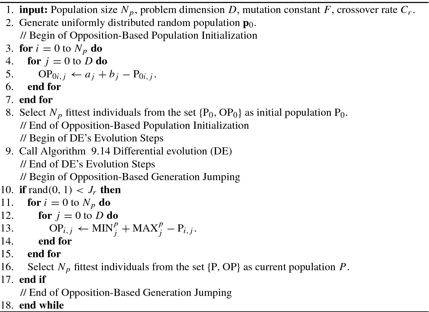
9.15.3 Two Variants of Opposition-Based Learning

In opposition-based learning, an opposite point is deterministically calculated with the reference point at the center in the fixed search range. There are two variants of opposite point selection.

The first variant is called quasi opposition-based learning (quasi-OBL), proposed in [130].

Definition 9.44 (Quasi-Opposite Number [130])

Let x be any real number between [a, b] and be its opposite number. The quasi-opposite number of x, denoted by x ^q, is defined as

(9.15.6)

where m = (a + b)∕2 is the middle of the interval [a, b] and rand(m, x ^o) is a random number uniformly distributed between m and the opposite point x ^o.

Definition 9.45 (Quasi-Opposite Point [130])

Let be any vector (point) in D-dimensional real space, and x _ij ∈ [a _j, b _j] for i = 1, …, N _p;j = 1, …, D. The quasi-opposite point of x _i, denoted by , is defined in its element form as

(9.15.7)

where i = 1, …, N _p;j = 1, …D, M _ij = (a _j + b _j)∕2 is the middle of the interval [a _j, b _j], and rand(M _ij, OP_ij) is a random number uniformly distributed between the middle M _ij and opposite number .

The calculation of the quasi-opposite point in (9.15.7) depends on the comparison of the values between the opposite-point and the original point as follows:

(9.15.8)

Figure 9.5 shows the opposite and quasi-opposite points of a solution (point) x.

Fig. 9.5

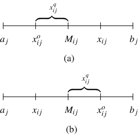
The opposite point and the quasi-opposite point. Given a solution with x _ij ∈ [a _j, b _j] and M _ij = (a _j + b _j)∕2, then and are the jth elements of the opposite point and the quasi-opposite point of x _i, respectively. (a) When x _ij > M _ij. (b) When x _ij < M _ij

Theorem 9.10 ([130])

Given a guess point , its opposite point and quasi opposite point , and given the distance from the solution d(⋅) and probability function P _r(⋅), then

(9.15.9)

The distance in the above theorem can take the Euclidean distance

(9.15.10)

or other distances.

Theorem 9.10 implies that for a black-box optimization problem (which means solution can appear anywhere over the search space), the quasi opposite point x ^q has a higher chance than the opposite point x ^o to be closer to the solution.

The quasi opposition-based learning consists of Quasi-Oppositional Population Initialization and Quasi-Oppositional Generation Jumping [130].

1. 1.
   Quasi-oppositional population initialization: Generate uniformly distributed random populations for i = 1, …, N _p, where for j = 1, …, D.

   • Compute the opposite populations associated with in element form:

     

     (9.15.11)
   • Denote the middle point between a _j and b _j as

     

     (9.15.12)
   • If letting the quasi-opposition of p _i be , then its elements are given by

     

     (9.15.13)

     Here, i = 1, …, N _p;j = 1, …, D.

   • Select N _p fittest individuals from the set as initial population p ⁰.

    
2. 2.
   Quasi-oppositional generation jumping: Let J _r be jumping rate, be minimum value of the jth individual in the current population, and denote maximum value of the jth individual in the current population.

   • If rand(0, 1) < J _r then calculate

     

     (9.15.14)
     

     (9.15.15)
     

     (9.15.16)

     Here, i = 0, …N _p − 1;j = 0, …, D − 1.

   • Select N _p fittest individuals from set the {P_ij, QOP_ij} as current population p.

    

If the oppositional population initialization and the oppositional generation jumping in Algorithm 9.19 are, respectively, replaced by the above quasi-oppositional population initialization and quasi-oppositional generation jumping, then the opposition-based differential evolution (ODE) described in Algorithm 9.19 becomes the quasi-oppositional differential evolution (QODE) in [130].

The second variant of the OBL is quasi reflection point-based OBL, which was proposed in [40].

Definition 9.46 (Quasi-Reflected Point [40])

Let be any point in D-dimensional real space, and x _ij ∈ [a _j, b _j]. Then the quasi-reflected point of x _i, denoted by , is defined in its element form as

(9.15.17)

where M _ij = (a _j + b _j)∕2, and rand(M _ij, x _ij) is a random number uniformly distributed between M _ij and x _ij.

Figure 9.6 shows the opposite, quasi-opposite, and quasi-reflected points of a solution (point) x _i.

Fig. 9.6

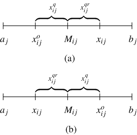
The opposite, quasi-opposite, and quasi-reflected points of a solution (point) x _i. Given a solution with x _ij ∈ [a _j, b _j] and M _ij = (a _j + b _j)∕2, then , , and are the jth elements of the opposite point , the quasi-opposite point , and the quasi-reflected opposite point of x _i, respectively. (a) When x _ij > M _ij. (b) When x _ij < M _ij

There are the following relations between the quasi-opposite point and quasi-reflected opposite point.

• The quasi-opposite point is generated by , whereas the quasi-reflected opposite point is defined by .

• The quasi-reflected opposite point is the mirror image of the quasi-opposite point with regard to the middle point M _ij, and hence is named as the quasi-reflected opposite point.

After calculating the fitness of opposite population generated by quasi-reflected opposition, the fittest N _p individuals in P and OP constitute the updated population. The application of the quasi-opposite points or the quasi-reflected opposite points will result into various variants and extensions of the basic OBL algorithm. For example, a stochastic opposition-based learning using a Beta distribution in differential evolution can be found in [121].

Brief Summary of This Chapter

• This chapter presents evolutionary computation tree.

• Evolutionary computation is a subset of artificial intelligence, which is essentially a computational intelligence for solving combinatorial optimization problems.

• Evolutionary computation, starting from a group of randomly generated individuals, imitates the biological genetic mode to update the next generation of individuals by replication, crossover, and mutation. Then, according to the size of fitness, the individual survival of the fittest improves the quality of the new generation of groups, after repeated iterations, gradually approaching the optimal solution. From the mathematical point of view, evolutionary computation is essentially a search optimization method.

• This chapter focuses on the Pareto optimization theory in multiobjective optimization problems existing in coevolutionary computation.

• Evolutionary computation has been widely used in artificial intelligence, pattern recognition, image processing, biology, electrical engineering, communication, economic management, mechanical engineering, and many other fields.

References

1. 1.
   Agrawal, R., Imielinski, T., Swami, A.N.: Mining association rules between sets of items in large databases. In: Proceedings of ACM SIGMOD International Conference on the Management of Data, pp. 207–216 (1992)
2. 2.
   Bäck, T., Hammel, U.: Evolution strategies applied to perturbed objective functions. In: Proceedings of 1st IEEE Conference Evolutionary Computation, vol. 1, pp. 40–45 (1994)
3. 3.
   Bäck, T., Schwefel H.-P.: An overview of evolutionary algorithms for parameter optimization. Evol. Comput. 1(1), 1–23 (1993)
4. 4.
   Baker, J.E.: Adaptive selection methods for genetic algorithms. In: Proceedings of the First International Conference on Genetic Algorithms and their Applications, Pittsburgh, pp. 101–111 (1985)
5. 5.
   Bandyopdhyay, S., Maulik, U.: An evolutionary technique based on K-means algorithm for optimal clustering in . Inform. Sci. 146(1–4), 221–237 (2002)
6. 6.
   Bandyopadhyay, S., Maulik, U., Holder, L.B., Cook, D.J.: Advanced Methods for Knowledge Discovery From Complex Data (Advanced Information and Knowledge Processing). Springer, London (2005)zbMATH
7. 7.
   Bandyopadhyay, S., Saha, S., Maulik, U., Deb, K.: A simulated annealing-based multiobjective optimization algorithm: AMOSA. IEEE Trans. Evol. Comput. 12(3), 269–283 (2008)
8. 8.
   Basu, M.: Dynamic economic emission dispatch using non-dominated sorting genetic algorithm-II. Electr. Power Energy Syst. 30, 140–149 (2008)
9. 9.
   Beckers, R., Deneubourg, J.L., Goss, S.: Trails and U-turns in the selection of the shortest path by the ant Lasius Niger. J. Theor. Biol. 159, 397–415 (1992)
10. 10.
    Benson, H.P., Sayin, S.: Towards finding global representations of the efficient set in multiple objective mathematical programming. Naval Res. Logist. 44, 47–67 (1997)MathSciNetzbMATH
11. 11.
    Bonabeau, E., Dorigo, M., Theraulaz, G.: Swarm Intelligence: From Natural to Artificial Systems. Oxford University Press, New York (1999)zbMATH
12. 12.
    Box, G.E.P.: Evolutionary operation: a method for increasing industrial productivity. Appl. Stat. VI(2), 81–101 (1957)
13. 13.
    Branke, J.: Multi-objective evolutionary algorithms and MCDA. European Working Group “Multiple Criteria Decision Aiding”, ser. 3, vol. 25, pp. 1–3 (2012)
14. 14.
    Branke, J., Schmidt, C., Schmeck, H.: Efficient fitness estimation in noisy environments. In: Proceedings of the Genetic and Evolutionary Computation, pp. 243–250 (2001)
15. 15.
    Bremermann, H.J.: Optimization through evolution and recombination. In: Yovits M.C., et al. (eds.) Self-Organizing Systems. Spartan, Washington (1962)
16. 16.
    Chang, D.X., Zhang, X.D., Zheng, C.W.: A genetic algorithm with gene rearrangement for K-means clustering. Pattern Recognit. 42, 1210–1222 (2009)
17. 17.
    Charnes, A., Cooper, W., Niehaus, R., Stredry, A.: Static and dynamic model with multiple objectives and some remarks on organisational design. Manag. Sci. 15B, 365–375 (1969)
18. 18.
    Chen, G., Low, C.P., Yang, Z.: Preserving and exploiting genetic diversity in evolutionary programming algorithms. IEEE Trans. Evol. Comput. 13(3), 661–673 (2009)
19. 19.
    Clerc, M., Kennedy, J.: The particle swarm - explosion, stability, and convergence in a multidimensional complex space. IEEE Trans. Evol. Comput. 6(1), 58–73 (2002)
20. 20.
    Coello Coello, C.A., Lamont, G.B., van Veldhuizen, D.A.: Evolutionary Algorithms for Solving Multi-Objective Problems (Genetic and Evolutionary Computation), 2nd edn. Springer, Berlin (2007)zbMATH
21. 21.
    Cordon, O., Herrera, F., Stutzle, T.: A review on the ant colony optimization metaheuristic: basis, models and new trends. Mathware Soft Comput. 9(2–3), 141–175 (2002)MathSciNetzbMATH
22. 22.
    Czyzak, P., Jaszkiewicz, A.: Pareto simulated annealing—a metaheuristic technique for multiple-objective combinatorial optimization. J. Multi-Crit. Decis. Anal. 7, 34–47 (1998)zbMATH
23. 23.
    Deb, K.: Multi-objective genetic algorithms: problem difficulties and construction of test problems. Evol. Comput. 7(3), 205–230 (1999)
24. 24.
    Deb, K.: Multi-Objective Optimization Using Evolutionary Algorithms. Wiley, London (2001)zbMATH
25. 25.
    Deb, K., Agarwal, S., Pratap, A., Meyarivan, T.: A fast and elitist multiobjective genetic algorithm: NSGA-II. IEEE Trans. Evol. Comput. 6(2), 182–197 (2002)
26. 26.
    del Valle, Y., Venayagamoorthy, G.K., Mohagheghi, S., Hernandez, J.-C., Harley, R.G.: Particle swarm optimization: basic concepts, variants and applications in power systems. IEEE Trans. Evol. Comput. 12(2), 171–195 (2008)
27. 27.
    Deneubourg, J.L., Aron, S., Goss, S., Pasteels, J.M.: The self-organizing exploratory pattern of the argentine ant. J. Insect Behav. 3, 159 (1990)
28. 28.
    Dorigo, M.: Optimization, learning and natural algorithms, Ph.D.Thesis, Politecnico diMilano (1992)
29. 29.
    Dorigo, M., Birattari, M.: Ant colony optimization. In: Sammut, C., Webb, G.I. (eds.) Encyclopedia of Machine Learning, pp. 37–40. Springer, Berlin (2011)
30. 30.
    Dorigo, M., Blumb, C.: Ant colony optimization theory: a survey. Theor. Comput. Sci. 344, 243–278 (2005)MathSciNetzbMATH
31. 31.
    Dorigo, M., Caro, G.D.: The ant colony optimization meta-heuristic. In: Corne, D., Dorigo, M, Glover, F. (eds.) New Ideas in Optimization, chap. 2. McGraw-Hill, New York (1999)
32. 32.
    Dorigo, M., Gambardella, L.M.: Ant colony system: a cooperative learning approach to the traveling salesman problem. IEEE Trans. Evol. Comput. 1(1), 53–66 (1997)
33. 33.
    Dorigo, M., Stützle, T.: The ant colony optimization metaheuristic: algorithms, applications, and advances. In: Glover, F., Kochenberger, G.A. (eds.) Handbook of Metaheuristics, chap. 9. Kluwer Academic, New York (2003)
34. 34.
    Dorigo, M., Maniezzo, V., Colorni, A.: The ant system: optimization by a colony of cooperating agents. IEEE Trans. Syst. Man Cybern. B 26(2), 29–41 (1996)
35. 35.
    Droste, S., Jansen, T., Wegener, I.: On the analysis of the (1 + 1) evolutionary algorithms. Theor. Comput. Sci. 276, 51–81 (2002)MathSciNetzbMATH
36. 36.
    Eberhart, R., Kennedy, J.: A new optimizer using particle swarm theory. In: Proceedings of the 6th International Symposium on Micro Machine and Human Science (MHS), pp. 39–43 (1995)
37. 37.
    Eberhart, R., Shi, Y., Kennedy, J.: Swarm Intelligence. Morgan Kaufmann, San Francisco (2001)
38. 38.
    Engelbrecht, A.P.: Particle swarm optimization: where does it belong? In: Proceedings of the 2003 IEEE Swarm Intelligence Symposium, pp. 48–54 (2006)
39. 39.
    Engrand, P.: A multi-objective approach based on simulated annealing and its application to nuclear fuel management. In: 5th International Conference on Nuclear Engineering, Nice, pp. 416–423 (1997)
40. 40.
    Ergezer, M., Simon, D., Du, D.: Oppositional biogeography-based optimization. In: Proceedings of IEEE International Conference on Systems, Man and Cybernetics (SMC), San Antonio, pp. 1009–1014 (2009)
41. 41.
    Fogel, L.J.: Autonomous automata. Ind. Res. 4, 14–19 (1962)
42. 42.
    Fogel, D.B.: An introduction to simulated evolutionary optimization. IEEE Trans. Neural Netw. 5, 3–14 (1994)
43. 43.
    Fogel, D.B.: Evolutionary Computation: Toward a New Philosophy of Machine Intelligence. IEEE Press, Piscataway (1995)zbMATH
44. 44.
    Fogel, L.J., Owens, A.J., Walsh, M.J.: Artificial Intelligence Through Simulated Evolution. Wiley, New York (1966)zbMATH
45. 45.
    Fonseca, C.M., Fleming, P.J.: An overview of evolutionary algorithms in multiobjective optimization. Evol. Comput. 3(1), 1–16 (1995)
46. 46.
    Friedberg, R.M.: A learning machine: part I. IBM J. 2(1), 2–13 (1958)MathSciNet
47. 47.
    Friedberg, R.M., Dunham, B., North, J.H.: A learning machine: part II. IBM J. 3(7), 282–287 (1959)MathSciNet
48. 48.
    Gao, W.F., Liu, S.Y.: Improved artificial bee colony algorithm for global optimization. Inf. Process. Lett. 111(17), 871–882 (2011)MathSciNetzbMATH
49. 49.
    Gao, W.F., Liu, S.Y., Huang, L.L.: A novel artificial bee colony algorithm based on modified search equation and orthogonal learning. IEEE Trans. Cybern. 43(3), 1011–1024 (2013)
50. 50.
    Geman, A., Geman, D.: Stochastic relaxation, Gibbs distributions, and the Bayesian restoration of images. IEEE Trans. Pattern Anal. Mach. Intell. 6(6), 721–741 (1984)zbMATH
51. 51.
    Gendreau, M., Potvin, J.-Y.: Metaheuristics in combinatorial optimization. Ann. Oper. Res. 140(1), 189–213 (2005)MathSciNetzbMATH
52. 52.
    Glover, F.: Tabu search — Part I. ORSA J. Comput. 1, 190–206 (1989)zbMATH
53. 53.
    Goh, C.K., Tan, K.C.: An investigation on noisy environments in evolutionary multiobjective optimization. IEEE Trans. Evol. Comput. 11(3), 354–381 (2007)
54. 54.
    Goldberg, D.E.: Genetic Algorithms in Search, Optimization, and Machine Learning. Addison-Wesley, Reading (1989)zbMATH
55. 55.
    Goldberg, D.E., Holland, J.H.: Genetic algorithms and machine learning. Mach. Learn. 3(2), 95–99 (1988)
56. 56.
    Goldberg, D.E., Richardson, J.: Genetic algorithms with sharing for multimodal function optimization. In: Proceedings of the Second International Conference on Genetic Algorithms on Genetic Algorithms and Their Application, Cambridge, pp. 41–49 (1987)
57. 57.
    Gong, Y.-J., Li, J.-J., Zhou, Y., Li, Y.,, Chung, H.S., Shi, Y.-H., Zhang, J.: Genetic learning particle swarm optimization. IEEE Trans. Cybern. 46(10), 2277–2290 (2016)
58. 58.
    Gong, D., Sun, J., Miao, Z.: A set-based genetic algorithm for interval many-objective optimization problems. IEEE Trans. Evol. Comput. 22(1), 47–60 (2018)
59. 59.
    Grasse, P.P.: La reconstruction du nid et les coordinations interindividuelles chez bellicositermes natalensis et cubitermes sp. la theorie de la stigmergie: Essai dinterpretation du comportement des termites constructeurs. Insectes Sociaux 6, 41–81 (1959)
60. 60.
    Hajek, B.: Hitting-time and occupation-time bounds implied by drift analysis with applications. Adv. Appl. Probab. 14(3), 502–525 (1982)MathSciNetzbMATH
61. 61.
    Hajela, P., Lin, C.-Y.: Genetic search strategies in multicriterion optimal design. Struct. Optim. 4, 99–107 (1992)
62. 62.
    Han, J., Kamber, M.: Data Mining: Concepts and Techniques. Morgan Kaufmann, San Francisco (2000)zbMATH
63. 63.
    Hans, A.E.: Multicriteria optimization for highly accurate systems. In: Stadler, W. (ed.) Multicriteria Optimization in Engineering and Sciences, Mathematical concepts and methods in science and engineering, vol. 19, pp. 309–352. Plenum Press, New York (1988)
64. 64.
    Hansen, M.P., Jaszkiewicz, A.: Evaluating the quality of approximations to the non-dominated set. Technical Report IMM-REP-1998-7, Technical University of Denmark (1998)
65. 65.
    Hastings, W.K.: Monte Carlo sampling methods using Markov chains and their applications. Biometrika 57(1), 97–109 (1970)MathSciNetzbMATH
66. 66.
    He, J., Yao, X.: Drift analysis and average time complexity of evolutionary algorithms. Artif. Intell. 127(1), 57–85 (2001)MathSciNetzbMATH
67. 67.
    He, J., Yao, X.: Erratum to: drift analysis and average time complexity of evolutionary algorithms. Artif. Intell. 140, 245–248 (2002)zbMATH
68. 68.
    Holland, J.H.: Outline for a logical theory of adaptive systems. J. Assoc. Comput. Mach. 3, 297–314 (1962)zbMATH
69. 69.
    Holland, J.H.: Adaption in Natural and Artificial Systems. University of Michigan Press, Ann Arbor (1975)zbMATH
70. 70.
    Hoorfar, A.: Mutation-based evolutionary algorithms and their applications to optimization of antennas in layered media. In: Proceedings of IEEE Antennas and Propagation Society International Symposium, Orlando, pp. 2876–2879 (1999)
71. 71.
    Hoorfar, A.: Evolutionary programming in electromagnetic optimization: a review. IEEE Trans. Antennas Propag. 55(3), 523–537 (2007)
72. 72.
    Hoorfar, A., Liu, Y.: A study of Cauchy and Gaussian mutation operators in evolutionary programming optimization of antenna structures. In: Proceedings of 16th Annual Applied Computational Electromagnetics Conference, Monterey, pp. 63–69 (2000)
73. 73.
    Horn, J.: Multicriterion decision making. In: Bäck, T., Fogel, D., Michalewicz, Z. (eds.) Handbook of Evolutionary Computation, vol. 1, pp. F1.9:1–F1.9:15. Oxford University Press, Oxford (1997)
74. 74.
    Horn, J., Nafpliotis, N., Goldberg, D.E.: A niched Pareto genetic algorithm for multiobjective optimization. In: Proceedings of the First IEEE Conference on Evolutionary Computation, IEEE World Congress on Computational Intelligence, vol. 1, pp. 82–87. IEEE Press, Piscataway (1994)
75. 75.
    Hughes, E.J.: Evolutionary multi-objective ranking with uncertainty and noise. In: Proceedings of first International Conference on Evolutionary Multi-Criterion Optimization, Zürich, pp. 329–343 (2001)
76. 76.
    Hughes, E.J.: Constraint handling with uncertain and noisy multi-objective evolution. In: Proceedings of 2001 Congress on Evolutionary Computation, vol. 2, pp. 963–970 (2001)
77. 77.
    Hutter, M., Legg, S.: Fitness uniform optimization. IEEE Trans. Evol. Comput. 10(5), 568–589 (2006)
78. 78.
    Hwang, C.-L., Masud, A.S.M.: Multiple Objective Decision Making-Methods and Applications. Springer, Berlin (1979)zbMATH
79. 79.
    Ishibuchi, H., Akedo, N., Nojima, Y.: Behavior of multiobjective evolutionary algorithms on many-objective knapsack problems. IEEE Trans. Evol. Comput. 19(2), 264–283 (2015)
80. 80.
    Jensen, M.T.: Reducing the run-time complexity of multiobjective EAs: the NSGA-II and other algorithms. IEEE Trans. Evol. Comput. 7(5), 503–515 (2003)
81. 81.
    Karaboga, D.: An idea based on honey bee swarm for numerical optimization. Erciyes University, Kayseri, Tech. Rep.-TR06 (2005)
82. 82.
    Karaboga, D., Basturk, B.: A powerful and efficient algorithm for numerical function optimization: artificial bee colony (ABC) algorithm. J. Global Optim. 39, 459–471 (2007)MathSciNetzbMATH
83. 83.
    Karaboga, D., Basturk, B.: On the performance of artificial bee colony (ABC) algorithm. Appl. Soft Comput. 8(1), 687–697 (2008)
84. 84.
    Karaboga, D., Basturk, B.: A comparative study of artificial bee colony algorithm. Appl. Math. Comput. 214(1), 108–132 (2009)MathSciNetzbMATH
85. 85.
    Kennedy, J.: Swarm intelligence. In: Zomaya, A.Y. (ed.) Handbook of Nature-Inspired and Innovative Computing, pp. 187–219. Springer, New York (2006)
86. 86.
    Kennedy, J., Eberhart, R.: Particle swarm optimization. In: Proceedings of IEEE International Conference on Neural Networks (ICNN), vol. IV, pp. 1942–1948 (1995)
87. 87.
    Kim, J.-H., Han, J.-H., Kim, Y.-H., Choi, S.-H., Kim, E.-S.: Preference-based solution selection algorithm for evolutionary multiobjective optimization. IEEE Trans. Evol. Comput. 16(1), 20–34 (2012)
88. 88.
    Kirkpatrick, S., Gelatt, C.D., Vecchi, M.P.: Optimization by simulated annealing. Science 220, 671–680 (1983)MathSciNetzbMATH
89. 89.
    Knowles, J.D., Corne, D.W.: On metrics for comparing nondominated sets. In: Proceedings of the Congress on Evolutionary Computation, vol. 1, pp. 711–716 (2002)
90. 90.
    Kursawe, F.: A variant of evolution strategies for vector optimization. In: Schwefel, H.-P., Manner, R. Parallel Problem Solving from Nature, 193–197. Springer, Berlin (1991)
91. 91.
    Laarhoven, P.J.M., Aarts, E.H.L.: Simulated Annealing: Theory and Applications. Reidel, Dordrecht (1987)zbMATH
92. 92.
    Laumanns, M., Rudolph, G., Schwefel, H.-P.: Mutation control and convergence in evolutionary multi-objective optimization. In: Proceedings of the 7th International Mendel Conference on Soft Computing (MENDEL 2001), Brno (2001)
93. 93.
    Li, H., Zhang, Q.: Multiobjective optimization problems with complicated Pareto sets, MOEA/D and NSGA-II. IEEE Trans. Evol. Comput. 13(2), 284–302 (2009)
94. 94.
    Li, Y.-L., Zhou, Y.-R., Zhan, Z.-H., Zhang, J.: A primary theoretical study on decomposition-based multiobjective evolutionary algorithms. IEEE Trans. Evol. Comput. 20(4), 563–576 (2016)
95. 95.
    Liao, T., Socha, K., Montes, M.A., Stützle, T., Dorigo, M.: Ant colony optimization for mixed-variable optimization problems. 18(4), 503–518 (2014)
96. 96.
    Limbourg, P., Aponte, D.E.S.: An optimization algorithm for imprecise multi-objective problem function. In: Proceedings of IEEE Congress on Evolutionary Computation, Edinburgh, pp. 459–466 (2005)
97. 97.
    López-Ioán̄ez, M., Stützle, T.: The automatic design of multiobjective ant colony optimization algorithms. IEEE Trans. Evol. Comput. 16(6), 861–875 (2012)
98. 98.
    Luo, B., Zheng, J., Xie, J., Wu, J.: Dynamic crowding distance - a new diversity maintenance strategy for MOEAs. In: Fourth International Conference on Natural Computation, pp. 580–585 (2008)
99. 99.
    Martens, D., Backer, M.D., Haesen, R., Vanthienen, J., Snoeck, M., Baesens, B.: Classification with ant colony optimization. IEEE Trans. Evol. Comput. 11(5), 651–665 (2007)
100. 100.
     Metropolis, N., Rosenbluth, A.W., Rosenbluth, M.N., Teller, A.H., Teller, E.: Equations of state calculations by fast computing machines. J. Chem. Phys. 21(6), 1087–1092 (1953)zbMATH
101. 101.
     Mezura-Montes, E., Velázquez-Reyes, J., Coello, C.A.C.: A comparative study of differential evolution variants for global optimization. In: Proceedings of the 2006 Conference on Genetic and Evolutionary Computation (GECCO-2006), Seattle, pp. 485–492 (2006)
102. 102.
     Michalewicz, Z.: Genetic Algorithms+Data Structures= Evolution Programs. AI Series. Springer, New York (1994)
103. 103.
     Miettinen, K.: Nonlinear Multiobjective Optimization. Kluwer, Norwell (1999)zbMATH
104. 104.
     Mitra, D., Romeo, F., Sangiovanni-Vincentelli, A.: Convergence and finite-time behavior of simulated annealing. Adv. Appl. Probab. 18, 747–771 (1986)MathSciNetzbMATH
105. 105.
     Mohan, B.C., Baskaran, R.: A survey: ant colony optimization based recent research and implementation on several engineering domain. Exp. Syst. Appl. 39, 4618–4627 (2012)
106. 106.
     Moradi, P., Gholampour, M.: A hybrid particle swarm optimization for feature subset selection by integrating a novel local search strategy. Appl. Soft Comput. 43, 117–130 (2016)
107. 107.
     Morse, J.N.: Reducing the size of the nondominated set: pruning by clustering. Comput. Oper. Res. 7(1–2), 55–66 (1980)
108. 108.
     Moulton, C.M., Roberts, S.A., Calatn, P.H.: Hierarchical clustering of multiobjective optimization results to inform land-use decision making. URISA J. 21(2), 25–38 (2009)
109. 109.
     Mühlenbein, H., Schlierkamp-Voosen, D.: The science of breeding and its application to the breeder genetic algorithm (BGA). Evol. Comput. 1(4), 335–360 (1994)
110. 110.
     Mukhopadhyay, A., Maulik, U., Bandyopadhyay, S., Coello Coello, C.A.: A survey of multiobjective evolutionary algorithms for data mining: part I. IEEE Trans. Evol. Comput. 18(1), 4–19 (2014)
111. 111.
     Mullen, R.J., Monekosso, D., Barman, S., Remagnino, P.: A review of ant algorithms. Exp. Syst. Appl. 36, 9608–9617 (2009)
112. 112.
     Myung, H., Kim, J.-H.: Hybrid evolutionary programming for heavily constrained problems. BioSystems 38, 29–43 (1996)
113. 113.
     Myung, H., Kim, J.-H., Fogel, D.B.: Preliminary investigations into a two-stage method of evolutionary optimization on constrained problems. In: McDonnell, J.R., Reynolds, R.G., Fogel, D.B. (eds.) Proceedings of the Fourth Annual Conference Evolutionary Programming, pp. 449–463. MIT Press, Cambridge (1995)
114. 114.
     Nam, D.K., Park, C.H.: Multiobjective simulated annealing: a comparative study to evolutionary algorithms. Inf. J. Fuzzy Syst. 2(2), 87–97 (2000)
115. 115.
     Neto, R.F.T., Filho, M.G.: A software model to prototype ant colony optimization algorithms. Exp. Syst. Appl. 38, 249–259 (2011)
116. 116.
     Nikulin, Y., Miettinen, K., Mäkelä, M.M.: A new achievement scalarizing function based on parameterization in multiobjective optimization. OR Spectr. 34, 69–87 (2012)MathSciNetzbMATH
117. 117.
     Oberkampf, W.L., Helton, J.C., Joslyn, C.A., Wojtkiewicz, S.F., Ferson, S.: Challenge problems: uncertainty in system response given uncertain parameters. Reliab. Eng. Syst. Saf. 85, 11–19 (2004)
118. 118.
     Osman, I.H., Laporte, G.: Metaheuristics: a bibliography. Ann. Oper. Res. 63(5), 511–623 (1996)zbMATH
119. 119.
     Palakonda, V., Mallipeddi, R.: Pareto dominance-based algorithms with ranking methods for many-objective optimization. IEEE Access 5, 11043–11053 (2017)
120. 120.
     Papadimitriou, C.H., Steiglitz, K.: Combinatorial Optimization: Algorithms and Complexity. Dover, New York (1982)zbMATH
121. 121.
     Park, S.-Y., Lee, J.-J.: Stochastic opposition-based learning using a Beta distribution in differential evolution. IEEE Trans. Cybern. 46(10), 2184–2194 (2016)
122. 122.
     Parpinelli, R.S., Lopes, H.S., Freitas, A.A.: Data mining with an ant colony optimization algorithm. IEEE Trans. Evol. Comput. 6(4), 321–332 (2002)zbMATH
123. 123.
     Premalatha, K., Natarajan, A.M.: Hybrid PSO and GA for global maximization. Int. J. Open Problems Compt. Math. 2(4), 597–608 (2009)MathSciNet
124. 124.
     Price, K., Storn, R., Lampinen, J.: Differential Evolution: A Practical Approach to Global Optimization. Springer, Berlin (2005)zbMATH
125. 125.
     Qin, A.K., Suganthan, P.N.: Self-adaptive differential evolution algorithm for numerical optimization. In: Proceedings of the 2005 IEEE Congress on Evolutionary Computation, vol. 2, pp. 1785–1791 (2005)
126. 126.
     Quagliarella, D., Vicini, A.: Coupling genetic algorithms and gradient based optimization techniques. In: Quagliarella, D., Periaux, J., Poloni, C., Winter, G. (eds.) Genetic Algorithms and Evolution Strategy in Engineering and Computer Science – Recent Advances and Industrial Applications. Wiley, Chichester (1997)zbMATH
127. 127.
     Radcliffe, N., Surry, P.: Fitness variance of formae and performance prediction. In: Foundations of Genetic Algorithms 3, pp. 51–72. Morgan Kaufmann, San Mateo (1995)
128. 128.
     Rahnamayan, S.: Opposition-based differential evolution. Thesis for Doctor of Philosophy, University of Waterloo (2007)
129. 129.
     Rahnamayan, S., Wang, G.G.: Center-based sampling for population-based algorithms. In: 2009 IEEE Congress on Evolutionary Computation, pp. 933–938 (2009)
130. 130.
     Rahnamayan, S., Tizhoosh, H.R., Salama, M.: Quasi-oppositional differential evolution. In: Proceedings of the IEEE Congress on Evolutionary Computation (CEC), Singapore, pp. 2229–2236 (2007)
131. 131.
     Rahnamayan, S., Tizhoosh, H.R., Salama, N.M.M.: Opposition-based differential evolution. IEEE Trans. Evol. Comput. 12(1), 64–79 (2008)
132. 132.
     Rakshit, P., Konar, A.: Differential evolution for noisy multiobjective optimization. Artif. Intell. 227, 165–189 (2015)MathSciNetzbMATH
133. 133.
     Rechenberg, I.: Cybernetic solution path of an experimental problem. Royal Aircraft Establishment, Library translation No. 1122, Farnborough, Hants (1965)
134. 134.
     Revelle, C., Cohon, J.L., Shobys, D.: Multiple objectives in facility location: a review. In: Beckmann, M., Kunzi, A.P. (eds.) Lecture Notes in Economics and Mathematical Systems, vol. 190, pp. 321–337. Springer, Berlin (1981)
135. 135.
     Rojas-Morales, N., Riff Rojas, M.-C., Ureta, E.M.: A survey and classification of opposition-based metaheuristics. Comput. Ind. Eng. 110, 424–435 (2017)
136. 136.
     Rosenthal, R.E.: Principles of multiobjective optimization. Decis. Sci. 16, 133–152 (1985)
137. 137.
     Ruiz, F., Luque, M., Miguel, F., del Mar Muñoz, M.: An additive achievement scalarizing function for multiobjective programming problems. Eur. J. Oper. Res. 188(3), 683–694 (2008)MathSciNetzbMATH
138. 138.
     Sakri, S., Rashid, N.A., Zain, Z.M.: Particle swarm optimization feature selection for breast cancer recurrence prediction. IEEE Access 6, 29637–29647 (2018)
139. 139.
     Santana, R.A., Pontes, M.R., Bastos-Filho, C.J.A.: A multiple objective particle Swarm optimization approach using crowding distance and roulette wheel. In: Ninth International Conference on Intelligent Systems Design and Applications, pp. 237–242 (2009)
140. 140.
     Sastry, K., Goldberg, D., Kendall, G.: Genetic algorithms. In: Burke, E.K., Kendall, G. (eds.) Search Methodologies: Introductory Tutorials in Optimization and Decision Support Techniques. Springer, New York (2005)
141. 141.
     Schaffer, J.D.: Multiple objective optimization with vector evaluated genetic algorithms. In: Proceedings of the First International Conference on Genetic Algorithms (ICGA’85), pp. 93–100 (1985)
142. 142.
     Schapire, R.E.: The strength of weak learnability. Mach. Learn. 5, 197–227 (1990)
143. 143.
     Schwefel, H.P.: Numerical Optimization of Computer Models. Wiley, Hoboken (1981)zbMATH
144. 144.
     Slater, M.: Lagrange multipliers (revisited). Cowles Commission Discussion Paper: Mathematics 403 (1950)
145. 145.
     Smith, K., Everson, R., Fieldsend, J.: Dominance measures for multi-objective simulated annealing. In: Proceedings of the 2004 IEEE Congress on Evolutionary Computation, pp. 23–30 (2004)
146. 146.
     Srinivas, N., Deb, K.: Multiobjective optimization using nondominated sorting in genetic algorithms. Evol. Comput. 2(3), 221–248 (1995)
147. 147.
     Storn, R., Price, K.: Differential evolution - a simple and efficient heuristic for global optimization over continuous spaces. J. Global Optim. 11, 341–359 (1997)MathSciNetzbMATH
148. 148.
     Tan, P.-N., Kumar, V., Srivastava, J.: Selecting the right interestingness measure for association patterns. In: Proceedings of the 8th ACM SIGKDD International Conference on KDD, pp. 32–41 (2002)
149. 149.
     Tang, K., Li, X., Suganthan, P.N., Yang, Z., Weise, T.: Benchmark functions for the CEC’2010 special session and competition on large-scale global optimization. Tech. Rep. (2009)
150. 150.
     Teich, J.: Pareto-front exploration with uncertain objectives. In: Zitzler, E. et al. (eds.) Evolutionary Multi-Criterion Optimization (EMO) 2001. Lecture Notes in Computer Science, vol. 1993, pp. 314–328 (2001)MathSciNet
151. 151.
     Tizhoosh, H.R.: Opposition-based learning: a new scheme for machine intelligence. In: Proceedings of the International Conference on Computational Intelligence for Modelling, Control and Automation, and International Conference on Intelligent Agents, Web Technologies and Internet Commerce, 28–30 November, Vienna, vol. 1, pp. 695–701 (2005)
152. 152.
     Ulungu, E.L., Teghem, J.: Multi-objective combinatorial optimization problems: a survey. J. MultiCrit. Decis. Anal. 3, 83–101 (1994)zbMATH
153. 153.
     Ulungu, E.L., Teghem, J., Fortemps, P., Tuyttens, D.: MOSA method: a tool for solving multiobjective combinatorial optimization problems. J. MultiCrit. Decis. Anal. 8, 221–236 (1999)zbMATH
154. 154.
     van den Bergh, F., Engelbrecht, A.P.: A cooperative approach to particle swarm optimization. IEEE Trans. Evol. Comput. 8(3), 225–239 (2004)
155. 155.
     Van Veldhuizen, D.A., Lamont, G.B.: Multiobjective evolutionary algorithms: analyzing the state-of-the-art. Evol. Comput. 8(2), 125–147 (2000)
156. 156.
     Wang, R., Zhang, Q., Zhang, T.: Decomposition-based algorithms using Pareto adaptive scalarizing methods. IEEE Trans. Evol. Comput. 20(6), 821–837 (2016)
157. 157.
     Whitley, D.: The GENITOR algorithm and selection pressure: why rank-based allocation of reproductive trials is best. In: Proceedings of the Third International Conference on Genetic Algorithms, San Mateo, pp. 116–123 (1989)
158. 158.
     Wierzbicki, A.P.: The use of reference objectives in multiobjective optimization. In: Fandel, G., Gal, T. (eds.) Multiple Criteria Decision Making Theory and Applications. MCDM Theory and Applications Proceedings. Lecture Notes in Economics and Mathematical Systems, vol. 177. Springer, Berlin, pp. 468–486 (1980)
159. 159.
     Wierzbicki, A.P.: A methodological approach to comparing parametric characterizations of efficient solutions. In: Fandel, G. et al. (eds.) Large-Scale Modeling and Interactive Decision Analysis. Lecture Notes in Economics and Mathematical Systems, vol. 273, pp. 27–45. Springer, Berlin (1986)
160. 160.
     Wierzbicki, A.P.: On the completeness and constructiveness of parametric characterizations to vector optimization problems. OR Spectr. 8, 73–87 (1986)MathSciNetzbMATH
161. 161.
     Xu, Q., Wang, L., Wang, N., Hei, X., Zhao, L.: A review of opposition-based learning from 2005 to 2012. Eng. Appl. Artif. Intell. 29, 1–12 (2014)
162. 162.
     Yang, Z., He, J., Yao, X.: Making a difference to differential evolution. In: Michalewicz, Z., Siarry, P. (eds.) Advances in Metaheuristics for Hard Optimization, pp. 397–414. Springer, Berlin (2008)
163. 163.
     Yang, L., Guan, Y., Sheng, W.: A novel dynamic crowding distance based diversity maintenance strategy for MOEAs. In: Proceedings of the 2017 International Conference on Machine Learning and Cybernetics, Ningbo, pp. 211–216 (2017)
164. 164.
     Yang, D., Liu, Z., Shu, T., Yang, L., Ouyang, J., Shen, Z.: An improved genetic algorithm for multiobjective optimization of helical coil electromagnetic launchers. IEEE Trans. Plasma Sci. 46(1), 127–133 (2018)
165. 165.
     Yao, X., Liu, Y., Lin, G.: Evolutionary programming made faster. IEEE Trans. Evol. Comput. 3(2), 82–102 (1999)
166. 166.
     Yao, X., Liu, Y., Lin, G.: Self-adaptive differential evolution with neighborhood search. In: Proceedings of the 2008 Congress on Evolutionary Computation (CEC2008), pp. 1110–1116 (2008)
167. 167.
     Zhang, Q., Li, H.: MOEA/D: a multiobjective evolutionary algorithm based on decomposition. IEEE Trans. Evol. Comput. 11(6), 712–731 (2007)
168. 168.
     Zhu, G.P., Kwong, S.: Gbest-guided artificial bee colony algorithm for numerical function optimization. Appl. Math. Comput. 217(7), 3166–3173 (2010)MathSciNetzbMATH
169. 169.
     Zitzler, E., Thiele, L.: Multiobjective optimization using evolutionary algorithms - a comparative case study. In: Eiben, V.A.E. et al. (eds.) Parallel Problem Solving From Nature. Springer, Berlin, 292–301 (1998)
170. 170.
     Zitzler, E., Thiele, L.: Multiobjective evolutionary algorithms: a comparative case study and the strength Pareto approach. IEEE Trans. Evol. Comput. 3(4), 257–271 (1999)
171. 171.
     Zitzler, E., Deb, K., Thiele, L.: Comparison of multiobjective evolutionary algorithms: empirical results. Evol. Comput. 8(2), 173–195 (2000)
172. 172.
     Zitzler, E., Laumanns, M., Thiele, L.: SPEA2: improving the strength Pareto evolutionary algorithm for multiobjective optimization. In: Proceedings of the Evolutionary Methods for Design, Optimization and Control with Applications to Industrial Problems (EUROGEN), pp. 95–100 (2002)
173. 173.
     Zitzler, E., Thiele, L., Laumanns, M., Fonseca, C.M., Fonseca, V.G.: Performance assessment of multiobjective optimizers: an analysis and review. IEEE Trans. Evol. Comput. 7(2), 117–132 (2003)