15.1 Introduction
In bilevel optimization one typically assumes that one has scalar-valued objective functions in the two levels of the bilevel program. This may be, for instance, costs, or time which has to be minimized. However, many real world problems can only be modeled adequately by considering several, in most cases conflicting, objective functions simultaneously, as weight and stability, or costs and time.
This occurs for instance in transportation planning [51]. We illustrate this with an example, cf. [17]. Let us consider a city bus transportation system financed by the public authorities. They have as target the reduction of the money losses in this non-profitable business. As a second target they want to motivate as many people as possible to use the buses instead of their own cars, as it is a public mission to reduce the overall traffic. The public authorities can decide about the bus ticket price, but this will influence the customers in their usage of the buses. The public has several, possibly conflicting, objectives, too, as to minimize their transportation time and costs. Hence, the usage of the public transportation system can be modeled on the lower level with the bus ticket price as parameter and with the solutions influencing the objective values of the public authorities on the upper level. Thus, such a problem can be modeled by multiobjective bilevel optimization.
In [17, 40] also a problem in medical engineering was discussed. There, the task was the configuration of coils. In the original version, this problem was a usual scalar-valued standard optimization problem which had to be reformulated as a bilevel optimization problem due to the need of real-time solutions and because of its structure. It turned out that the engineers would accept—or even prefer—solutions which do not satisfy a previous equality constraint strictly in favor of incorporating some additional objectives. This led to the examination of two objective functions on both levels.
Dempe and Mehlitz consider in [11] a bilevel control problem, where the three objective functions are approximating a given target state as good as possible, minimizing the overall control effort, and the sparcity of the chosen control.
In case we have more than one objective function then we speak of a multiobjective optimization problem. Collecting for instance m objective functions in an m-dimensional vector also leads to the name vector optimization, as now vector-valued maps have to be optimized. In case we have a bilevel program with a vector-valued objective on one or both of the levels we speak of a multiobjective bilevel optimization problem. In case one has multiple functions just on one level one also uses the name semivectorial bilevel problem.
For instance, Pilecka studies in [39] bilevel optimization problems with a single-objective lower level and a vector-valued function on the upper level. The same structure was assumed by Gadhi and Dempe in [23, 24] or Ye in [50]. Bonnel and co-authors [3] study semivectorial bilevel problems with a multiobjective optimization problem on the lower level. For optimality conditions for bilevel problems with such a structure (multiobjective on the lower level, single-objective on the upper level), see also Dempe and co-authors in [12].
In this chapter we will give a short introduction to multiobjective optimization. First, an optimality concept for such optimization problems has to be formulated. By doing that, one can define stricter or weaker concepts, which may have advantages from applications point of view or from the theoretical or numerical point of view, respectively.
We give scalarization results and optimality conditions which allow to characterize the set of optimal solutions of a multiobjective optimization problem. We also point out some of the developments on numerical solvers. Throughout the chapter we emphasize more on nonlinear problems. For the linear case of a multiobjective bilevel optimization problem with multiple functions on each level see for instance [9] and the references therein. We will also study reformulations of the feasible set of the upper level problem, which can be used to formulate numerical solution approaches.
In bilevel optimization also multiple objectives arise: a function on the upper level and a function on the lower level. Hence, we will also discuss the relationship between multiobjective and bilevel optimization from this perspective.
15.2 Basics of Multiobjective Optimization
As we will consider bilevel optimization problems with a multiobjective optimization problem on the lower or/and on the upper level, we start by giving an overview on the main optimality notions typically used in multiobjective optimization.

 (
( ) and a nonempty set of feasible points
  .
. . A set K is a convex cone if λ(x + y) ∈ K for all λ ≥ 0, x, y ∈ K, and K is a pointed convex cone if additionally K ∩ (−K) = {0}. A partial ordering introduced by a pointed convex cone is antisymmetric. The partial ordering is then defined by
 be a closed pointed convex cone.
 we have for

 . For more details on ordering structures in vector optimization we refer to [21].
By using the concept of a partial ordering, we are now able to define two types of optimal solutions of (MOP)


Of course, any efficient point is also weakly efficient, in case int(K) ≠ ∅. Whenever we speak of weakly efficient points, we assume that the ordering cone K has a nonempty interior. We denote the set of all K-minimal points, i. e. of all efficient points, as  , and the set of all weakly efficient points as
  . The set
  is called nondominated set and the set
  weakly nondominated set.
 the efficient points are also denoted as Edgeworth-Pareto (EP)-minimal points. Then the definition can also be formulated as follows: a point
  is an EP-minimal point for (MOP) if there is no x ∈ Ω with
 if there is no x ∈ Ω with
![$$\displaystyle \begin{aligned}f_i(\lambda\, x+(1-\lambda)\,y)<\lambda\,f_i(x)+(1-\lambda)\,f_i(y)\ \mbox{ for all }\ x,y\in\Omega,\ x\neq y,\ \lambda\in]0,1[,\end{aligned}$$](../images/480569_1_En_15_Chapter/480569_1_En_15_Chapter_TeX_Equg.png)
 is also an efficient point of (MOP) w.r.t.
  .
.For iterative numerical approaches, the following result is useful: in case the feasible set becomes larger and one has already determined the efficient points of the smaller set, then this can be used for determining the efficient points w.r.t. a larger superset.
 , and a vector-valued function
 , consider the sets

Let f(A
0) be compact. Then it holds
 .△
.△
For numerical calculations, also the notion of ε-minimal solutions can be useful. We state here a definition for the ordering cone  , see also for instance [30, 31, 48]:
 with ε
i > 0, i = 1, …, m, be given. A point
with ε
i > 0, i = 1, …, m, be given. A point  is an ε-EP-minimal solution of the multiobjective optimization problem (MOP) if there is no x ∈ Ω with
 ,
,  be defined by f(x) = x for all
  and
and  . Then the set of efficient points is


 is an ε-EP-minimal solution of the multiobjective optimization problem minx ∈ Ωf(x) but not an efficient point.
For multiobjective optimization problems also more general optimality notions have been introduced, which use more general ordering structures. For instance, Ye discusses in [50] semivectorial bilevel problems where the preference relation is locally satiated and almost transitive. Moreover, the concept of using a fixed ordering cone can be replaced by using an ordering map which associates to each element y of the space an ordering cone K(y). This was done by Dempe and Gadhi in [10]. They study semivectorial bilevel problems with a multiobjective optimization problem on the upper level and where the cones K(y) are assumed to be Bishop-Phelps-cones. For such multiobjective optimization problems also proper nonlinear scalarizations exist, see [19], which have also been used by Dempe and Gadhi in their approach for formulating necessary optimality conditions. Variable ordering structures have been intensively studied, cf. [18] and, within the context of set-optimization, in [20]. There is a strong relation between bilevel optimization and set optimization, i.e. with optimization with a set-valued objective function. This arises whenever the optimal solution set on the lower level is not unique, see [39].
15.3 Characterization of Optimal Solutions of a Multiobjective Optimization Problem
For solving problem (MOP) several methods are discussed in the literature. For surveys see [13, 29, 35, 42]. An often used approach is to replace the vector optimization problem by a suitable scalar-valued optimization problem. This fact is also used in numerical methods for multiobjective bilevel problems to reformulate the lower level problem by a single-objective problem or by the optimality conditions of this reformulation.


 we have
  and
and  .
.For convex multiobjective optimization problems one can use linear scalarization for a full characterization of the weakly efficient points.


△
Hence, in the convex case, we have a full characterization of weakly efficient points. A similar result as in (b) does not exist for efficient points and for K #. This is shown with the next example.
 with f(x) = x,
  , and
, and  . Then
 there exists no
  with
with 
 is a minimal solution of

 . Such linear scalarizations are also called weighted-sum approach, and the components w
i of the vector w ∈ K
∗ are interpreted as weights of the objective function.
. Such linear scalarizations are also called weighted-sum approach, and the components w
i of the vector w ∈ K
∗ are interpreted as weights of the objective function.The approach in (15.3.1) is for instance used in [32, 33]. The authors reformulate a linear semivectorial bilevel programming problem (with a multiobjective optimization problem on the lower level) as a special bilevel programming problem, where the lower level is a parametric linear scalar-valued optimization problem. For characterizing the set in (15.3.1) optimality conditions from scalar-valued optimization can be used. This approach with using the weighted sum is also examined in [11] and it is pointed out that this is a delicate issue in case one studies locally optimal solutions of the parameterized problem only.
 which satisfies all objective functions equally good and is better with respect to one of the objective functions. By considering instead the set
Theorem 15.3.1(b) requires the set f( Ω) + K to be convex. This holds in case the functions f
i are convex,  , and Ω is a convex set. For nonconvex multiobjective optimization problems one has to use nonlinear scalarizations. A widely used one is a scalarization by Pascoletti and Serafini, [38], also known as Tammer-Weidner-functional [26, 27]. This scalarization approach allows to determine weakly efficient points for an arbitrary ordering cone K while many other well known nonlinear scalarizations as the ε-constraint problem (see [13, 28, 34, 35]) are mainly developed for determining EP-minimal points, only. Moreover, those can also be seen as a special case of the Pascoletti-Serafini-scalarization, see [15]. Thus, results gained for the Pascoletti-Serafini problem can be applied to these scalarization problems, too.

 to the multiobjective optimization problem (MOP). The main properties of this scalarization approach are the following:


△
Thus all efficient points of the multiobjective optimization problem can be found even for non-convex problems by choosing suitable parameters. We are even able to restrict the choice of the parameter a to a hyper plane in the image space according to the following theorem ([16], Theorem 3.2).
Let
 and r ∈ K be given. We define a hyper plane H by
 with
with
 . Then there is a parameter a ∈ H and some
 such that
 is a minimal solution of the problem (15.3.2).△
Also other scalarizations are used for deriving results on multiobjective bilevel optimization problems. For instance, Gadhi and Dempe use in [23] the scalarization known as signed-distance functional for deriving optimality conditions. This functional evaluates the distance of a point to the negative of the ordering cone as well as to the complement of the negative of the ordering cone.
We end this section by giving the KKT-type (i.e., Karush-Kuhn-Tucker-type) optimality conditions for constrained multiobjective optimization problems. KKT-conditions, and optimality conditions in general, are often used to characterize the optimal solutions of the lower level of a bilevel optimization problem. Such an approach was for instance named to be a classical approach by Deb and Sinha in [6] and it was used by Chuong in [4] for a nonsmooth multiobjective bilevel optimization problem. As it is known from single-objective optimization, KKT-conditions typically include complementarity conditions which are difficult to handle mathematically. Moreover, the necessary conditions require some regularity assumptions (cf. (A2) in [33]). For more details on the sufficiency and necessity of the optimality conditions we refer for instance to [13, 29].
 , k = 1, …, p be continuously differentiable functions such that
We give in the following the necessary conditions which also hold for just locally efficient solutions, too. For a proof see for instance [13, Theorem 3.21].
 be a weakly efficient solution of (MOP) and assume that there exists some
 such that

 and
and
 such that

△
Under appropriate convexity assumptions we can also state sufficient conditions. We state here a simplified version. For weaker assumptions on the convexity of the functions, as quasiconvexity for the constraints, we refer to [29].
Let Ω be given as in (15.3.3) and let f
j, j = 1, …, m and g
k, k = 1, …, p be convex and continuously differentiable. Let
 and assume that there exist Lagrange multipliers
 and
and
 such that (15.3.4) is satisfied. Then,
 is a weakly efficient solution of (MOP).△
15.4 Connection Between Multiobjective Optimization and Bilevel Optimization
In bilevel optimization one has (at least) two objective functions: one on the upper and one on the lower level. In multiobjective optimization one also studies problems with two or more objective functions. This naturally leads to the question on how these problem classes are related, and whether bilevel problems can be reformulated as multiobjective optimization problems. This question was answered for nonlinear problems by Fliege and Vicente in [22]: only by introducing a very special order relation the optimal solutions of the bilevel problem are exactly the efficient points of a multiobjective optimization problem. Only for continuously differentiable problems on the lower level this order relation can be formulated as a more tractable order relation. We give some of the basic ideas in the following, all based on [22]. For a more recent survey and unifying results as well as a more general characterization of the connections between single-level and bilevel multiobjective optimization we refer to [41]. They also provide a thorough literature survey on this topic as well as the historic sources of this approach for bilevel linear problems.

 are the upper-level and lower-level objective functions respectively. Hence, we assume that there are no constraints in each level and we assume the optimistic approach. The handling of constraints is also shortly described in [22].
As a related multiobjective optimization problem, it is not enough to study just a problem with the vector-valued function (f u(x u, x ℓ), f ℓ(x u, x ℓ)), as counter examples, which can be found in the literature, demonstrate. Instead, a possibility to give a relation is to use a map which includes the vector x u as a component. But still, it is not enough to use the standard componentwise partial ordering. The authors in [22] present a complete reformulation with an ordering which is not numerically tractable. They also formulate a weaker relation which we present in the following but which gives a sufficient condition only.
 defined by


then
 is an optimal solution of the bilevel optimization problem (15.4.1).△
The study about the relation between multiobjective and bilevel optimization problems is also continued and unified in [41] as already mentioned above. The authors also study thereby multiobjective bilevel optimization problems and their connection to multiobjective optimization. A thorough exploration of the use of these relations for numerical approaches for bilevel problems is an open research topic.
15.5 A Multiobjective Bilevel Program
In this section, we introduce the multiobjective bilevel optimization problem. We formulate the general bilevel optimization problem (see (15.5.3)). Then we introduce the so-called optimistic approach (see (15.5.4)) which is a special case of the general bilevel optimization problem. Next, we give a possibility on how to describe the feasible set of such an optimistic bilevel problem as the solution set of a specific multiobjective optimization problem. This will be used in Sect. 15.6 within a numerical method. Then, with an example, we illustrate again what might happen in case the lower level problem has not a unique solution, now in the setting that there is only one objective function on the lower level but several on the upper level.
Moreover, we mention a typical approach from the literature, namely scalarization. We discuss what happens in case one considers weakly efficient points of the lower level problem instead of efficient ones, which is often done when using scalarizations. We end the section by introducing coupling constraints between the upper and the lower level.
 of the upper level. In case of multiple objectives, this lower level problems reads as
 and a set
  (
( ). The constraint (x, y) ∈ G can be replaced by
 of this lower level problem are called lower level variables. For a constant
  , let x(y) be a minimal solution of (15.5.1), hence

 ,
,  , and a compact set
  . Here, the constraint
  is uncoupled from the lower level variable. An even more general formulation of the bilevel problem is reached by allowing the constraint
  to depend on the lower level variable x, what we will discuss shortly later. We speak of a multiobjective bilevel optimization problem if m
1 ≥ 2 or m
2 ≥ 2.
to depend on the lower level variable x, what we will discuss shortly later. We speak of a multiobjective bilevel optimization problem if m
1 ≥ 2 or m
2 ≥ 2.If the minimal solution of the lower level problem (15.5.1) is not unique, i. e. the set Ψ(y) consists of more than one point, the objective function F(x(⋅), ⋅) is not well-defined for  . That is the reason why the word
  is written in quotes in (15.5.3). This difficulty is in some works avoided by just assuming that the solution of the lower level problem is unique. But in the case of a multiobjective optimization problem (m
1 ≥ 2) on the lower level this is in general not reasonable any more.
is written in quotes in (15.5.3). This difficulty is in some works avoided by just assuming that the solution of the lower level problem is unique. But in the case of a multiobjective optimization problem (m
1 ≥ 2) on the lower level this is in general not reasonable any more.


Thus, in the optimistic modification (15.5.4), the objective function of the upper level is minimized w. r. t. x and y, while in the general formulation (15.5.3) it is only minimized w. r. t. the upper level variable y. In the following, we consider the optimistic approach only, i. e. the bilevel optimization problem as in (15.5.4).
When assuming this optimistic approach, one assumes at the same time that the decision maker on the lower level allows the decision maker on the upper level to utilize any solution from the set of efficient points of the lower level, which might not be realistic. See also the discussion in [45, 47].
In [45], also the case where the lower level decision maker has sufficient power to make a deterministic decision from the set of efficient points of the lower level is studied. This is formulated by using a value function on the objective functions of the lower level, which needs to be known in this setting. By using a value function the lower level problem is somehow reduced to a single-objective problem. To overcome the difficulty of determining the lower level value function, Sinha and co-authors suggest in [46] to handle uncertainties in the lower level value function.
 and for the lower level by the closed pointed convex cone
  . For the case m
1 ≥ 2 the set Ψ(y) is the solution set of a multiobjective optimization problem w. r. t. the ordering cone K
1. Thus, using (15.5.2), we write instead of x ∈ Ψ(y)
. For the case m
1 ≥ 2 the set Ψ(y) is the solution set of a multiobjective optimization problem w. r. t. the ordering cone K
1. Thus, using (15.5.2), we write instead of x ∈ Ψ(y) 
 the set of K
1-minimal points of the multiobjective optimization problem (15.5.1) parameterized by y. Hence we study
the set of K
1-minimal points of the multiobjective optimization problem (15.5.1) parameterized by y. Hence we study 

 -minimal points of the multiobjective optimization problem

 is thus an element of the set of feasible points Ω if and only if it is a
  -minimal point of the multiobjective optimization problem (15.5.7). This is shown in the following theorem. There is also a close relation to the reformulation using the function F in (15.4.2), see [41].
Let
 be the set of
 -minimal points of the multiobjective optimization problem (15.5.7) with
 . Then it holds
 .△
.△

A multiobjective bilevel optimization problem is a quite challenging problem in case there are multiple objectives on each level, as just discussed. But already in case there are only multiple objectives on the upper level, such semivectorial bilevel problems become quite difficult. This is even more the case when the lower level problem does not have unique optimal solutions. We illustrate this with an example taken from [39, Ex. 4.14]. This example also gives insight to the optimistic approach.

![$$\displaystyle \begin{aligned}\Psi(y)= \left\{ \begin{array}{ll} ]-\infty, 1]& \mbox{ if }\ y=0,\\ {} [0,1]& \mbox{ if }\ y\in]0,1]. \end{array}\right. \end{aligned}$$](../images/480569_1_En_15_Chapter/480569_1_En_15_Chapter_TeX_Equac.png)
![$$\displaystyle \begin{aligned}\begin{array}{c} \mathrm{'}\min\limits_{y\in\mathbb{R}}\mathrm{'}\, F(x(y),y)\\ \mbox{subject to the contraints}\\ x(y)\in \Psi(y),\\ y\in [0,1] \end{array} \end{aligned}$$](../images/480569_1_En_15_Chapter/480569_1_En_15_Chapter_TeX_Equad.png)


![$$\displaystyle \begin{aligned}\tilde F(y)= \left\{ \begin{array}{ll} \mbox{conv}(\{(-1,0),(0,-1)\})\cup \{(u,0)\mid u\in ]-\infty,-1]\}& \mbox{ if }\ y=0\\ {} \mbox{conv}(\{(-y-1,y),(-y,y-1)\})& \mbox{ if }\ y=]0,1] \end{array}\right. \end{aligned}$$](../images/480569_1_En_15_Chapter/480569_1_En_15_Chapter_TeX_Equag.png)
 with
with ![$$\hat x\in \Psi (1)=[0,1]$$](../images/480569_1_En_15_Chapter/480569_1_En_15_Chapter_TeX_IEq97.png) and
and  is not an optimal solution of the optimistic formulation
 ![$$\displaystyle \begin{aligned}\begin{array}{c} \min\limits_{x,y} F(x(y),y)\\ \mbox{subject to the contraints}\\ x(y)\in \Psi(y),\\ y\in [0,1]. \end{array} \end{aligned}$$](../images/480569_1_En_15_Chapter/480569_1_En_15_Chapter_TeX_Equah.png)
 , i.e. by solving a set optimization problem, as proposed in [39, p. 60], there would also be solutions with
  . This is a hint that studying bilevel problems with non-unique lower-level-optimal solutions by using techniques from set optimization might lead to other solutions, which might also be of interest.
 , Lv and Wan use in [32, 33] a weighted-sum approach, as discussed in Sect. 15.3, to characterize the optimal solutions of the lower level in case the lower level problem is convex and some regularity assumptions are satisfied. For the theoretical verification see Theorem 15.3.1. Then, instead of (15.5.6), they study

As done in these reformulations, many authors take the weakly efficient elements instead of the efficient, i.e. they replace the condition  from the lower level problem by
  . The next example shows that this can have a strong impact. We use for this examples ideas from [11].
![$$\displaystyle \begin{aligned}\begin{array}{c} \min\limits_{x,y} x+2y\\ \mbox{subject to the constraints} \\ x\in\Psi(y)=\mbox{argmin} \left\{ (xy, 1-x)\mid x\in[0,1] \right\},\\ y\in [0,1]. \end{array} \end{aligned}$$](../images/480569_1_En_15_Chapter/480569_1_En_15_Chapter_TeX_Equak.png)
![$$\displaystyle \begin{aligned}\Psi(y)=\left\{ \begin{array}{ll} \{1\}&\mbox{ if }y=0,\\ {[} 0, 1 {]}&\mbox{ if }y\in ( 0 , 1 ]. \end{array} \right. \end{aligned}$$](../images/480569_1_En_15_Chapter/480569_1_En_15_Chapter_TeX_Equal.png)
![$$\displaystyle \begin{aligned}\Psi^w(y)=[0,1]\ \mbox{ for }\ y\in[0,1]\end{aligned}$$](../images/480569_1_En_15_Chapter/480569_1_En_15_Chapter_TeX_Equam.png)
Instead of enlarging the feasible set by taking the weakly efficient solutions instead of the efficient solutions, one could also use the so-called properly efficient solutions, which are a subset of the efficient solutions. Those can completely be characterized by linear scalarizations, at least in the convex case, by using elements w ∈ K #. Such an approach was discussed by Gebhardt and Jahn in [25]. The advantage is that the gained optimal values of the bilevel problem are then upper bounds on the optimal values of the original problem, and, what is more, that the gained optimal solutions are in fact feasible for the original problem, as any properly efficient solution is also efficient.

 . This results in a coupling of the upper level variable y and the lower level variable x. Then
First notice that the constraint  from the upper level cannot just be moved to the lower level as simple examples, see for instance [14, Example 7.4], show. This has also a practical interpretation. The same constraint on the lower level restricting the constraint set on the lower level has a different meaning as on the upper level. There, the feasibility is restricted after the determination of the minimal solution of the lower level and is thus an implicit constraint. For more details see [8, pp. 25].
A generalization of the results from Theorem 15.5.1 is not possible as discussed in [14, Chapter 7]. We also illustrate this with the following example.
![$$\displaystyle \begin{aligned}\begin{array}{c} \min\limits_{y\in\mathbb{R}} F(x,y)= \left(\begin{array}{c}x_1-y \\x_2\end{array}\right) \\ {} \mbox{subject to the constraints} \\[1.5ex] x=x(y)\in \mbox{argmin}_{x\in\mathbb{R}^2}\bigg\{ f(x,y)= \left( \begin{array}{c} x_1\\x_2 \end{array} \right) \bigg|\ (x,y)\in G\bigg\},\\[2.5ex] (x,y)\in\tilde G \end{array} \end{aligned}$$](../images/480569_1_En_15_Chapter/480569_1_En_15_Chapter_TeX_Equao.png)
 , m
1 = m
2 = 2,
, m
1 = m
2 = 2, 


 be the set of (
 )-minimal points of the tricriteria optimization problem
 ![$$\displaystyle \begin{aligned}\begin{array}{c} \min\limits_{x,y} \left(\begin{array}{c}x_1 \\x_2\\y\end{array}\right) \\ {} \mbox{subject to the constraints} \\[1.5ex] (x,y)\in G\cap \tilde G=\{(x,y)\in\mathbb{R}^3\mid 0\leq y\leq 1,\ x_1+x_2\geq -1,\ \|x\|{}_2^2\leq y^2\} \end{array} \end{aligned}$$](../images/480569_1_En_15_Chapter/480569_1_En_15_Chapter_TeX_Equat.png)
 (cf. [14, Theorem 7.5]) we show that it does not hold
  .
.


![$$\displaystyle \begin{aligned}\begin{array}{rl} & \left(\begin{array}{c} \bar x_1 \\ \bar x_2 \\ \bar y \end{array} \right)\in \left\{\left( \begin{array}{c} x_1 \\ x_2 \\ y \\ \end{array} \right)\right\}+(\mathbb{R}^2_+\times\{0\})\setminus\{0\}\\ \\[0.5ex] \Leftrightarrow &\left( \begin{array}{c} \bar x_1 \\ \bar x_2 \\ \end{array} \right)\in \left\{\left( \begin{array}{c} x_1 \\ x_2 \\ \end{array} \right)\right\}+\mathbb{R}^2_+\setminus\{0\}\ \wedge\ y=\bar y. \end{array} \end{aligned}$$](../images/480569_1_En_15_Chapter/480569_1_En_15_Chapter_TeX_Equau.png)


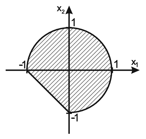

![$$\displaystyle \begin{aligned}\mathcal{S}^{\min}=\bigg\{ (x_1,x_2,y)\ \bigg|\ x_1=-1-x_2,\ x_2=-\frac{1}{2}\pm\frac{1}{4}\sqrt{8y^2-4}, y\in\left[\frac{\sqrt{2}}{2}\,,\,1\right] \bigg\}.\end{aligned}$$](../images/480569_1_En_15_Chapter/480569_1_En_15_Chapter_TeX_Equav.png)
 of this set is
 ![$$\displaystyle \begin{aligned}\bigg\{(z_1,z_2)\in\mathbb{R}^2\,\bigg|\, z_1=-1-z_2-y,\ z_2=-\frac{1}{2}\pm\frac{1}{4}\sqrt{8y^2-4}, y\in\left[\frac{\sqrt{2}}{2}\,,\,1\right]\bigg\}.\end{aligned}$$](../images/480569_1_En_15_Chapter/480569_1_En_15_Chapter_TeX_Equaw.png)
Solution set  of the biobjective bilevel optimization problem of Example 15.5 and the image
15.6 Numerical Methods
As stated in the introduction, we concentrate in this chapter on nonlinear problems. Procedures for solving linear multiobjective bilevel problems are presented e. g. in [36].
Much less papers are dealing with nonlinear multiobjective bilevel problems: Shi and Xia [43, 44] present an interactive method, also using a scalarization (the ε-constraint scalarization, cf. [47]). Osman, Abo-Sinna et al. [1, 37] propose the usage of fuzzy set theory for convex problems. Teng et al. [49] give an approach for a convex multiperson multiobjective bilevel problem.
Bonnel and Morgan consider in [2] a semivectorial bilevel optimization problem and propose a solution method based on a penalty approach. However, no numerical results are given.
More recently, in [14, 17] Theorem 15.5.1 was used for developing a numerical algorithm. There, first the efficient set of the multiobjective optimization problem (15.5.7) was calculated (or at least approximated). According to Theorem 15.5.1, this efficient set equals the feasible set of the upper level problem of the original bilevel problem. As the efficient set of (15.5.7) was approximated by a finite set of points, these points can be evaluated and compared easily by the upper level function. The approximation of the efficient set of (15.5.7) is then iteratively refined around points which have had promising objective function values w.r.t. the upper level functions.
- 1.
Calculate an approximation of the efficient set of (15.5.7) w.r.t. the partial ordering defined by the cone
 . This is done by determining equidistant representations of the efficient sets of the multiobjective problems (15.5.1) for various discretization points y in the set
  .
. - 2.
Select all non-dominated points of the lower level problems being non-dominated for the upper level problem.
- 3.
Refine the approximation of the efficient set of the original problem by refining the approximation of the set of feasible points of the upper level problem.
 .
. ![$$\displaystyle \begin{aligned}\begin{array}{c} \min\limits_{x,y} \left(\begin{array}{c} F_1(x,y)\\ F_2(x,y) \end{array}\right)= \left(\begin{array}{c} x_1+x_2^2+y+\sin^2(x_1+y)\\ \cos{}(x_2)\cdot(0.1+y)\cdot\left(\exp(-\frac{\displaystyle x_1}{\displaystyle 0.1+x_2})\right) \end{array}\right)\\ \mbox{subject to the constraints} \\ x\in\mbox{argmin}_{x\in\mathbb{R}^2}\left\{ \left(\begin{array}{c}f_1(x,y)\\f_2(x,y)\end{array}\right) \mid (x,y)\in G\right\},\\ y\in[0,10] \end{array} \end{aligned}$$](../images/480569_1_En_15_Chapter/480569_1_En_15_Chapter_TeX_Equax.png)
 ,
, ![$$\displaystyle \begin{aligned}\begin{array}{rcl} f_1(x,y)&=&\frac{\displaystyle (x_1-2)^2+(x_2-1)^2}{\displaystyle 4}+ \frac{\displaystyle x_2y+(5-y)^2}{\displaystyle 16}+\sin\left(\frac{\displaystyle x_2}{\displaystyle 10}\right), \\[1.5ex] f_2(x,y)&=&\frac{\displaystyle x_1^2+(x_2-6)^4-2x_1y-(5-y)^2}{\displaystyle 80} \end{array}\end{aligned}$$](../images/480569_1_En_15_Chapter/480569_1_En_15_Chapter_TeX_Equay.png)

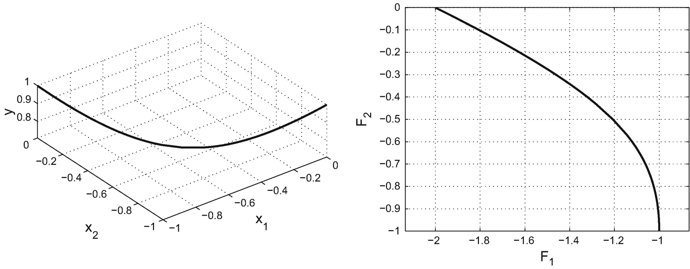
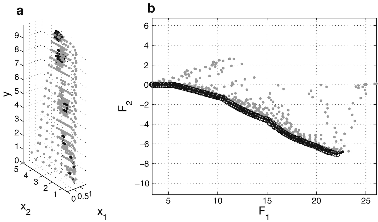
![$$\tilde G=[0,10]$$](../images/480569_1_En_15_Chapter/480569_1_En_15_Chapter_TeX_IEq126.png) , i.e. we choose y ∈{0, 0.6, 1.2, 1.8, …, 9.6, 10}. For example, for y = 1.8 one obtains the representation of the efficient set of problem (15.5.1) as shown in Fig. 15.3a. In the image space of the lower level problem this representation is shown in Fig. 15.3b.
, i.e. we choose y ∈{0, 0.6, 1.2, 1.8, …, 9.6, 10}. For example, for y = 1.8 one obtains the representation of the efficient set of problem (15.5.1) as shown in Fig. 15.3a. In the image space of the lower level problem this representation is shown in Fig. 15.3b.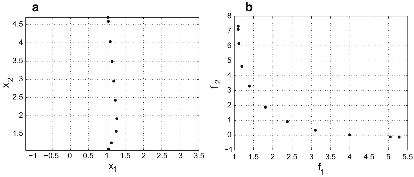
Representation (a) of the efficient set and (b) the nondominated set of problem (15.5.1) for y = 1.8
 are marked with circles and are connected with lines.
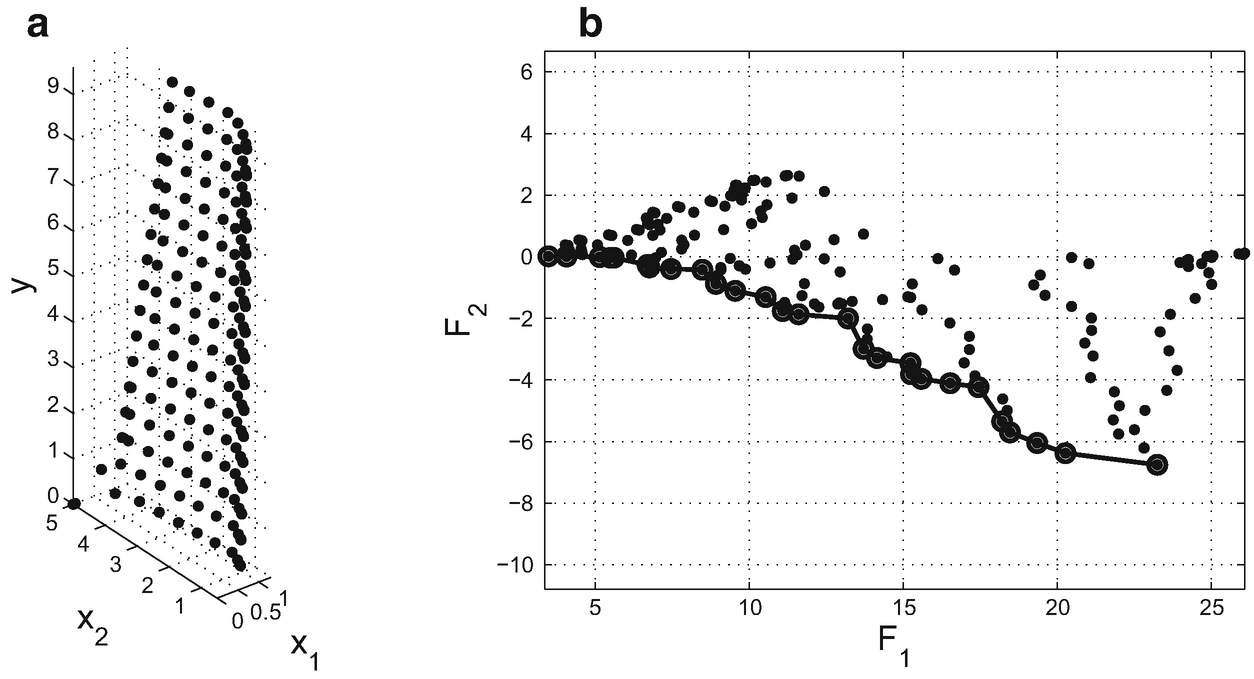
(a) Approximation A 0 of the set of feasible points Ω and (b) the image F(A 0) of this set under F
(a) Final approximation A f of the set of feasible points Ω and (b) the image F(A f) of this set under F
Later, another numerical deterministic approach for nonlinear problems was proposed by Gebhardt and Jahn in [25]. They propose to use a multiobjective search algorithm with a subdivision technique. The studied problems have multiple objectives on both levels. The authors also discuss optimality conditions for replacing the multiobjective problem on the lower level. Instead of taking the weakly efficient solutions of the lower level, they suggest to take the properly efficient solutions. By doing this the feasible set of the upper level gets smaller (instead of larger by using weakly efficient elements) and thus one gets upper bounds, and minimal solutions which are in fact feasible for the original problem. However, the authors do not use this for their numerical approach. Instead, the main ingredient of their algorithm is a subdivision technique for multiobjective problems which uses randomly generated points in boxes, where the size is decreased when the algorithm proceeds. It is assumed that the feasible set of the upper level variable  is such that one can easily work with a discretization of it, for instance an interval. Then the upper level variables are fixed to these values coming from the discretization, and the lower level problems are solved with an algorithm from the literature which uses subdivision techniques. While the procedure is appropriate only for small number of variables, it is capable of detecting globally optimal solutions also for highly nonlinear problems.
Also, the construction of numerical test instances is an important aspect. Test instances which are scalable in the number of variables and the number of objectives and where the set of optimal solutions are known are important to evaluate and compare numerical approaches. Deb and Sinha propose five of such test problems in [5]. For the test instances the optimistic approach is chosen.
There have also been some numerical approaches for solving bilevel multiobjective optimization problems by using evolutionary algorithms. An attempt is for instance given by Deb and Sinha in [6]. A hybrid solver combined with a local solver was proposed by the same authors in [7].