S. Dempe, A. Zemkoho (eds.)Bilevel OptimizationSpringer Optimization and Its Applications161https://doi.org/10.1007/978-3-030-52119-6_17

17. Bilevel Linear Optimization Under Uncertainty

Johanna Burtscheidt¹ and Matthias Claus¹

(1)

Faculty of Mathematics, University of Duisburg-Essen, Essen, Germany

Johanna Burtscheidt

Email: johanna.burtscheidt@uni-due.de

Matthias Claus (Corresponding author)

Email: matthias.claus@uni-due.de

Abstract

We consider bilevel linear problems, where the right-hand side of the lower level problems is stochastic. The leader has to decide in a here-and-now fashion, while the follower has complete information. In this setting, the leader’s outcome can be modeled by a random variable, which gives rise to a broad spectrum of models involving coherent or convex risk measures and stochastic dominance constraints. We outline Lipschitzian properties, conditions for existence and optimality, as well as stability results. Moreover, for finite discrete distributions, we discuss the special structure of equivalent deterministic bilevel programs and its potential use to mitigate the curse of dimensionality.

Keywords

Bilevel stochastic programmingLinearRisk measureStabilityDifferentiabilityDeterministic counterpart

17.1 Introduction

In this chapter we consider bilevel optimization models with uncertain parameters. Such models can be classified based on the chronology of decision and observation as well as the nature of the uncertainty involved. A bilevel stochastic program arises, if the uncertain parameter is realization of some random vector with known distribution, that can only be observed once the leader has submitted their decision. In contrast, the follower decides under complete information.

If upper and lower level objectives coincide, the bilevel stochastic program collapses to a classical stochastic optimization problem with recourse (cf. [1, Chap. 2]). Relations to other mathematical programming problems are explored in the seminal work [2] that also established the existence of solutions, Lipschitzian properties and directional differentiability of a risk-neutral formulation of a bilevel stochastic nonlinear model. Moreover, gradient descent and penalization methods were investigated to tackle discretely distributed stochastic mathematical programs with equilibrium constraints (SMPECs).

Reference [3] studies an application to topology optimization problems in structural mechanics. Many other applications are motivated by network related problems that inherit a natural order of successive decision making under uncertainty. Notable examples arise in telecommunications (cf. [4]), grid-based (energy) markets (cf. [5–8]) or transportation science (cf. [9, 10]). An extensive survey on bilevel stochastic programming literature is provided in [11, Chap. 1.4].

In two-stage stochastic bilevel programming leader and follower take two decisions: The decision on the respective first-stage variables is made in a here-and-now fashion, i.e. without knowledge of the realization of the random parameter. In contrast, the respective second-stage decisions are made in a wait-and-see manner, i.e. after observing the parameter (cf. [12]).

This chapter is organized as follows: In Sects. 17.2.1–17.2.5, we outline structural properties, existence and optimality conditions as well as stability results for bilevel stochastic linear problems while paying special attention to the modelling of risk-aversion via coherent or convex risk measures or stochastic dominance constraints. Sections 17.2.6 and 17.2.7 are devoted to the algorithmic treatment of bilevel stochastic linear problems, where the underlying distribution is finite discrete . An application of two-stage stochastic bilevel programming in the context of network pricing is discussed in Sect. 17.3. The chapter concludes with an overview of potential challenges for future research.

17.2 Bilevel Stochastic Linear Optimization

While the analysis in this section is confined to the bilevel stochastic linear problems with random right-hand side , the concepts and underlying principles can be easily transferred to stochastic extensions of more complex bilevel programming models.

17.2.1 Preliminaries

We consider the optimistic formulation of a parametric bilevel linear program

$\displaystyle \begin{aligned} \min_x \left\{c^\top x + \min_y \{q^\top y \; | \; y \in \Psi(x,z)\} \; | \; x \in X \right\}, \end{aligned}$

P(z)

where $X \subseteq \mathbb {R}^n$ is a nonempty polyhedron, $c \in \mathbb {R}^n$ and $q \in \mathbb {R}^m$ are vectors, $z \in \mathbb {R}^s$ is a parameter, and the lower level optimal solution set mapping $\Psi : \mathbb {R}^n \times \mathbb {R}^s \rightrightarrows \mathbb {R}^m$ is given by

$\displaystyle \begin{aligned}\Psi(x,z) := \underset{y}{\mbox{Argmin}} \; \{d^\top y \; | \; Ay \leq Tx + z\} \end{aligned}$

with matrices $A \in \mathbb {R}^{s \times m},\ T \in \mathbb {R}^{s \times n}$ and a vector $d \in \mathbb {R}^m$ . Let $f: \mathbb {R}^n \times \mathbb {R}^s \to \mathbb {R} \cup \lbrace \pm \infty \rbrace$ denote the mapping

$\displaystyle \begin{aligned}f(x,z) := c^\top x + \min_y \{q^\top y \; | \; y \in \Psi(x,z)\}. \end{aligned}$

Lemma 17.2.1

Assume dom f ≠ ∅, then f is real-valued and Lipschitz continuous on the polyhedron $P = \{(x,z) \in \mathbb {R}^n \times \mathbb {R}^s \; | \; \exists y \in \mathbb {R}^m: Ay \leq Tx + z\}$ . △

Proof

By Eaves [13, Sect. 3], ∅ ≠ dom f ⊆dom Ψ implies dom Ψ = P. Consequently, the linear program in the definition of f(x, z) is solvable for any (x, z) ∈ P by parametric linear programming theory (see [14, Sect. 2.3.2]). Consider any (x, z), (x′, z′) ∈ P. Without loss of generality, assume that f(x, z) ≥ f(x′, z′) and let y′∈ Ψ(x′, z′) be such that f(x′, z′) = c ^⊤x′ + q ^⊤y′. Following [15] we obtain

$\displaystyle \begin{aligned} \begin{array}{rcl} |f(x,z)-f(x',z')| \; &\displaystyle = \; f(x,z)- c^\top x' - q^\top y' \; \leq \; c^\top x + q^\top y - c^\top x' - q^\top y' \\ &\displaystyle \leq \; \|c\| \|x-x'\| + \|q\| \|y-y'\| \end{array} \end{aligned}$

for any y ∈ Ψ(x, z). Let $\mathbb {B}$ denote the Euclidean unit ball and 0 < Λ < ∞ a constant, then [16, Theorem 4.2] yields

$\displaystyle \begin{aligned}\Psi(x',z')\subseteq \Psi(x,z)+ \Lambda \|(x,z)-(x',z')\|\mathbb{B} \end{aligned}$

and hence |f(x, z) − f(x′, z′)| ≤ (∥c∥ + Λ∥q∥)∥(x, z) − (x′, z′)∥. □

Remark 17.2.2

An alternate proof for Lemma 17.2.1 is given in [17, Theorem 1]. However, the arguments above can be easily extended to lower level problems with convex quadratic objective function and linear constraints. △

Linear programming theory (cf. [18]) provides verifiable necessary and sufficient condition for dom f ≠ ∅:

Lemma 17.2.3

dom f ≠ ∅ holds if and only if there exists $(x,z) \in \mathbb {R}^n \times \mathbb {R}^s$ such that

a.
{y | Ay ≤ Tx + z} is nonempty,
b.
there is some $u \in \mathbb {R}^s$ satisfying A ^⊤u = d and u ≤ 0, and
c.
the function y↦q ^⊤y is bounded from below on Ψ(x, z).

Under these conditions,

$\displaystyle \begin{aligned}\min_{y} \lbrace q^\top y \; | \; y \in \Psi(x',z') \rbrace \end{aligned}$

is attained for any (x′, z′) ∈ P. △

17.2.2 Bilevel Stochastic Linear Programming Models

A bilevel stochastic program arises if the parameter z = Z(ω) in P(z) is the realization of a known random vector Z on some probability space $(\Omega , \mathcal {F}, \mathbb {P})$ and we assume the following chronology of decision and observation:

../images/480569_1_En_17_Chapter/480569_1_En_17_Eque_HTML.png

Throughout the analysis, we assume the stochasticity to be purely exogenous, i.e. the distribution of Z to be independent of x.

Let $\mu _Z := \mathbb {P} \circ Z^{-1} \in \mathcal {P}(\mathbb {R}^s)$ denote the Borel probability measure induced by Z. We shall assume dom f ≠ ∅ and that the lower level problem is feasible for any leader’s decision and any realization of the randomness, i.e.

$\displaystyle \begin{aligned}X \subseteq P_Z := \lbrace x \in \mathbb{R}^n \; | \; (x,z) \in P \; \forall z \in \mbox{supp} \; \mu_Z \rbrace. \end{aligned}$

In two-stage stochastic programming, a similar assumption is known as relatively complete recourse (cf. [1, Sect. 2.1.3]). In this setting, each leader’s decision x ∈ X gives rise to a random variable f(x, Z(⋅)). We thus may fix any mapping $\mathcal {R}: \mathcal {X} \to \mathbb {R}$ , where $\mathcal {X}$ is a linear subspace of $L^0(\Omega , \mathcal {F}, \mathbb {P})$ that contains the constants and satisfies

$\displaystyle \begin{aligned}\lbrace f(x,Z(\cdot)) \; | \; x \in X \rbrace \subseteq \mathcal{X}, \end{aligned}$

and consider the bilevel stochastic program

$\displaystyle \begin{aligned} \min_x \left\{\mathcal{R}[f(x,Z(\cdot))] \; | \; x \in X \right\}. \end{aligned}$

(17.2.1)

Under suitable moment or boundedness conditions on Z the classical L ^p-spaces $L^p(\Omega , \mathcal {F}, \mathbb {P})$ with p ∈ [1, ∞] are natural choices for the domain $\mathcal {X}$ of $\mathcal {R}$ . We define

$\displaystyle \begin{aligned}\mathcal{M}^p_s := \left\{ \mu \in \mathcal{P}(\mathbb{R}^s) \; | \; \int_{\mathbb{R}^s} \|z\|{}^p~\mu(dz) < \infty \right\}, \end{aligned}$

which denotes the set of Borel probability measures on $\mathbb {R}^s$ with finite moments of order p ∈ [1, ∞), and the set

$\displaystyle \begin{aligned}\mathcal{M}^\infty_s := \left\{ \mu \in \mathcal{P}(\mathbb{R}^s) \; | \; \mbox{supp} \; \mu_Z \; \text{is bounded} \right\}. \end{aligned}$

Lemma 17.2.4

Assume dom f ≠ ∅ and $\mu _Z \in \mathcal {M}^p_s$ for some p ∈ [1, ∞]. Then the mapping $F: P_Z \to L^0(\Omega , \mathcal {F}, \mathbb {P})$ given by F(x) := f(x, Z(⋅)) takes values in $L^p(\Omega , \mathcal {F}, \mathbb {P})$ and is Lipschitz continuous with respect to the L ^p-norm. △

Proof

We first consider the case that p is finite. By (0, 0) ∈ P and Lemma 17.2.1, there exist a constant L _f such that

$\displaystyle \begin{aligned} \begin{array}{rcl} \| F(x) \|{}_{L^p}^p &\displaystyle \leq 2^p |f(0,0)|{}^p + 2^p \int_{\mathbb{R}^s} |f(x,z) - f(0,0)|{}^p~\mu_Z(dz) \\ &\displaystyle \leq 2^p |f(0,0)|{}^p + 2^p L_f^p \|x\|{}^p + 2^p L_f^p \int_{\mathbb{R}^s} \|z\|{}^p~\mu_Z(dz) < \infty \end{array} \end{aligned}$

holds for any x ∈ P _Z. Furthermore, for any x, x′∈ P _Z we have

$\displaystyle \begin{aligned}\| F(x) - F(x') \|{}_{L^p} = \left( \int_{\mathbb{R}^s} |f(x,z) - f(x',z)|{}^p~\mu_Z(dz) \right)^{1/p} \leq L_f \|x - x' \|. \end{aligned}$

For p = ∞, Lemma 17.2.1 implies that for any fixed x ∈ P _Z, the mapping f(x, ⋅) is continuous on supp μ _Z. Thus, $\mu _Z \in \mathcal {M}^\infty _s$ yields

$\displaystyle \begin{aligned}\|F(x)\|{}_{L^\infty} \leq \sup_{z \in \mbox{supp} \; \mu_Z} |f(x,z)| < \infty.\end{aligned}$

Moreover, for any x, x′∈ P _Z we have

$\displaystyle \begin{aligned}\| F(x) - F(x') \|{}_{L^\infty} \leq \sup_{z \in \mbox{supp} \; \mu_Z} |f(x,z) - f(x',z)| \leq L_f \|x-x'\|.\end{aligned}$

□

The mapping $\mathcal {R}$ in (17.2.1) can be used to measure the risk associated with the random variable F(x).

Definition 17.2.5

A mapping $\mathcal {R}: \mathcal {X} \to \mathbb {R}$ defined on some linear subspace $\mathcal {X}$ of $L^0(\Omega , \mathcal {F}, \mathbb {P})$ containing the constants is called a convex risk measure if the following conditions are fulfilled:

a.
(Convexity) For any $Y_1, Y_2 \in \mathcal {X}$ and λ ∈ [0, 1] we have
$\displaystyle \begin{aligned}\mathcal{R}[\lambda Y_1 + (1-\lambda)Y_2] \leq \lambda \mathcal{R}[Y_1] + (1 - \lambda) \mathcal{R}[Y_2]. \end{aligned}$
b.
(Monotonicity) $\mathcal {R}[Y_1] \leq \mathcal {R}[Y_2]$ for all $Y_1, Y_2 \in \mathcal {X}$ satisfying Y ₁ ≤ Y ₂ with respect to the $\mathbb {P}$ -almost sure partial order.
c.
(Translation equivariance) $\mathcal {R}[Y + t] = \mathcal {R}[Y] + t$ for all $Y \in \mathcal {X}$ and $t \in \mathbb {R}$ .

A convex risk measure $\mathcal {R}$ is coherent if the following holds true:

d.
(Positive homogeneity) $\mathcal {R}[t Y] = t \cdot \mathcal {R}[Y]$ for all $Y \in \mathcal {X}$ and t ∈ [0, ∞). △

Definition 17.2.6

A mapping $\mathcal {R}: \mathcal {X} \to \mathbb {R}$ is called law-invariant if for all $Y_1, Y_2 \in \mathcal {X}$ with $\mathbb {P} \circ Y_1^{-1} = \mathbb {P} \circ Y_2^{-1}$ we have $\mathcal {R}[Y_1] = \mathcal {R}[Y_2]$ . △

Coherent risk measures have been introduced in [19], while the analysis of convex risk measures dates back to [20]. A thorough discussion of their analytical traits is provided in [21]. Below we list some risk measures that are commonly used in stochastic programming (cf. [1, Sect. 6.3.2]).

Examples

(a)
The expectation $\mathbb {E}: L^1(\Omega , \mathcal {F}, \mathbb {P}) \to \mathbb {R}$ ,
$\displaystyle \begin{aligned}\mathbb{E}[Y] = \int_\Omega Y(\omega)~\mathbb{P}(d\omega), \end{aligned}$

is a law-invariant and coherent risk measure that turns (17.2.1) into the risk neutral bilevel stochastic program
$\displaystyle \begin{aligned}\min_x \left\{\mathbb{E}[F(x)] \; | \; x \in X \right\}. \end{aligned}$
(b)
The expected excess of orderp ∈ [1, ∞) over a predefined level $\eta \in \mathbb {R}$ is the mapping $\mbox{EE}_{\eta }^p: L^p(\Omega , \mathcal {F}, \mathbb {P}) \to \mathbb {R}$ given by
$\displaystyle \begin{aligned}\mbox{EE}_{\eta}^p[Y] := \Big( \mathbb{E}\big[\max \lbrace Y - \eta, 0 \rbrace^p \big] \Big)^{1/p}. \end{aligned}$

$\mbox{EE}_{\eta }^p$ is law-invariant, convex and nondecreasing, but neither translation-equivariant nor positively homogeneous (cf. [1, Example 6.22]).
(c)
The mean upper semideviation of orderp ∈ [1, ∞) is the mapping $\mbox{SD}^p_\rho : L^p(\Omega , \mathcal {F}, \mathbb {P}) \to \mathbb {R}$ defined by
$\displaystyle \begin{aligned}\mbox{SD}_\rho^p[Y] := \mathbb{E}[Y] + \rho \cdot \mbox{EE}_{\mathbb{E}[Y]}^p[Y] = \mathbb{E}[Y] + \rho \cdot \Big( \mathbb{E}\big[\max \lbrace \mathbb{E}[Y] - \eta, 0 \rbrace^p \big] \Big)^{1/p}, \end{aligned}$

where ρ ∈ (0, 1] is a parameter. $\mbox{SD}_\rho ^p$ is a law-invariant coherent risk measure (cf. [1, Example 6.20]).
(d)
The excess probability $\mbox{EP}_\eta : L^0(\Omega , \mathcal {F}, \mathbb {P}) \to \mathbb {R}$ over a prescribed target level $\eta \in \mathbb {R}$ given by
$\displaystyle \begin{aligned}\mbox{EP}_\eta[Y] = \mathbb{P}[\lbrace \omega \in \Omega \; | \; Y(\omega) > \eta \rbrace], \end{aligned}$

is nondecreasing and law-invariant. However, it lacks convexity, translation-equivariance and positive homogeneity (cf. [22, Example 2.29]).
(e)
The Value-at-Risk $\mbox{VaR}_\alpha : L^0(\Omega , \mathcal {F}, \mathbb {P}) \to \mathbb {R}$ at level α ∈ (0, 1) defined by
$\displaystyle \begin{aligned}\mbox{VaR}_{\alpha}[Y] := \inf \lbrace \eta \in \mathbb{R} \; | \; \mathbb{P}[\lbrace \omega \in \Omega \; | \; Y(\omega) \leq \eta \rbrace] \geq \alpha \rbrace \end{aligned}$

is law-invariant, nondecreasing, translation-equivariant and positively homogeneous, but in general not convex (cf. [23]).
(f)
The Conditional Value-at-Risk $\mbox{CVaR}_\alpha : L^1(\Omega , \mathcal {F}, \mathbb {P}) \to \mathbb {R}$ at level α ∈ (0, 1) given by
$\displaystyle \begin{aligned}\mbox{CVaR}_{\alpha}[Y] := \inf \lbrace \eta + \frac{1}{1-\alpha}\mbox{EE}_{\eta}^1[Y] \; | \; \eta \in \mathbb{R} \rbrace \end{aligned}$

is a law-invariant coherent risk measure (cf. [23, Proposition 2]). The variational representation above was established in [24, Theorem 10].
(g)
The entropic risk measure $\mbox{Entr}_{\alpha }: L^\infty (\Omega , \mathcal {F}, \mathbb {P}) \to \mathbb {R}$ defined by
$\displaystyle \begin{aligned}\mbox{Entr}_{\alpha}[Y] := \frac{1}{\alpha} \ln \Big( \mathbb{E} \big[\exp(\alpha Y) \big] \Big), \end{aligned}$

where α > 0 is a parameter, is a law-invariant convex (but not coherent) risk measure (cf. [21, Example 4.13, Example 4.34]).
(h)
The worst-case risk measure $\mathcal {R}_{\max }: L^\infty (\Omega , \mathcal {F}, \mathbb {P}) \to \mathbb {R}$ given by
$\displaystyle \begin{aligned}\mathcal{R}_{\max}[Y] := \sup_{\omega \in \Omega} Y(\omega) \end{aligned}$

is law-invariant and coherent (cf. [21, Example 4.8]). This choice of $\mathcal {R}$ in (17.2.1) leads to the bilevel robust problem
$\displaystyle \begin{aligned}\min_x \left\{\mathcal{R}_{\max}[F(x)] \; | \; x \in X \right\}. \end{aligned}$

Note that $\mathcal {R}_{\max }$ only depends on the so called uncertainty set $Z(\Omega ) \subseteq \mathbb {R}$ . Thus, a bilevel robust problem can be formulated without knowledge of the distribution of the uncertain parameter. In robust optimization, the uncertainty set is often assumed to be finite, polyhedral or ellipsoidal (cf. [25]).

Remark 17.2.7

The set of convex (coherent) risk measures on $L^p(\Omega , \mathcal {F}, \mathbb {P})$ is a convex cone for any fixed p ∈ [1, ∞]. In particular, if $\mathcal {R}: L^p(\Omega , \mathcal {F}, \mathbb {P}) \to \mathbb {R}$ is a convex (coherent) risk measure, then so is $\mathbb {E} + \rho \cdot \mathcal {R}$ for any ρ ≥ 0. The mean-risk bilevel stochastic programming model

$\displaystyle \begin{aligned}\min_x \left\{\mathbb{E}[F(x)] + \rho \cdot \mathcal{R}[F(x)] \; | \; x \in X \right\} \end{aligned}$

seeks to minimize a weighted sum of the expected value of the outcome and a quantification of risk.△

Example

Consider the bilevel stochastic problem

$\displaystyle \begin{aligned}\min \left\{ \mathcal{R}[\min \Psi(x,Z)] \; | \; 1 \leq x \leq 6 \right\}, \end{aligned}$

where Ψ(x, z) := Argmin_y{−y | y ≥ 1, y ≤ x + 2 + z ₁, y ≤−x + 8.5 + z ₂} and assume that Z is uniformly distributed over the square [−0.5, 0.5]².

As it can be seen in Fig. 17.1, we have

$\displaystyle \begin{aligned}\Psi(x,z) = \begin{cases} \lbrace x + 2 +z_1 \rbrace &\text{if} \; x \leq 3.25 + 0.5z_2 - 0.5z_1 \\ \lbrace -x + 8.5 + z_2 \rbrace &\text{else} \end{cases} \end{aligned}$

for any x ∈ [1, 6] and z ∈ [−0.5, 0.5]². A straightforward calculation shows that

$\displaystyle \begin{aligned} \begin{array}{rcl} \mathbb{E}[\min \Psi(x,Z)] &\displaystyle = \int_{-0.5}^{0.5} \int_{-0.5}^{0.5} x + 2 + z_1~dz_1~dz_2 \\ &\displaystyle = x+2 \end{array} \end{aligned}$

holds for any x ∈ [1, 2.75]. Similarly, we have

$\displaystyle \begin{aligned} \begin{array}{rcl} \mathbb{E}[\min \Psi(x,Z)] &\displaystyle = \int_{-0.5}^{2x-6} \int_{-0.5}^{-2x + 6.5 + z_2} x + 2 + z_1~dz_1~dz_2 \\ &\displaystyle + \int_{2x-6}^{0.5} \int_{-0.5}^{0.5} x + 2 + z_1~dz_1~dz_2 \\ &\displaystyle +\int_{6-2x}^{0.5} \int_{-0.5}^{2x - 6.5 + z_1} -x + 8.5 + z_2~dz_2~dz_1 \\ &\displaystyle = -\frac{4}{3}x^3 + 11x^2 - \frac{117}{4} x + \frac{1427}{48} \end{array} \end{aligned}$

for x ∈ [2, 75, 3.25] and

$\displaystyle \begin{aligned} \begin{array}{rcl} \mathbb{E}[\min \Psi(x,Z)] &\displaystyle = \int_{2x-7}^{0.5} \int_{-0.5}^{-2x + 6.5 + z_2} x + 2 + z_1~dz_1~dz_2 \\ &\displaystyle +\int_{-0.5}^{7-2x} \int_{-0.5}^{2x - 6.5 + z_1} -x + 8.5 + z_2~dz_2~dz_1 \\ &\displaystyle +\int_{7-2x}^{0.5} \int_{-0.5}^{0.5} -x + 8.5 + z_2~dz_2~dz_1 \\ &\displaystyle = \frac{4}{3} x^3 - 15 x^2 + \frac{221}{4} x - \frac{989}{16} \end{array} \end{aligned}$

for x ∈ [3.25, 3.75]. Finally, for x ∈ [3.75, 6] we calculate

$\displaystyle \begin{aligned} \begin{array}{rcl} \mathbb{E}[\min \Psi(x,Z)] &\displaystyle = \int_{-0.5}^{0.5} \int_{-0.5}^{0.5} -x + 8.5 + z_2~dz_2~dz_1 \\ &\displaystyle = -x + 8.5. \end{array} \end{aligned}$

Thus, $\mathbb {E}[\min \Psi (\cdot \,,Z)]$ is piecewise polynomial, non-convex and non-differentiable . It is easy to check that x ^∗ = 6 is a global minimizer of the risk-neutral model

$\displaystyle \begin{aligned}\min \left\{ \mathbb{E}[\min \Psi(x,Z)] \; | \; 1 \leq x \leq 6 \right\}. \end{aligned}$

In this particular example, x ^∗ is also a global minimizer of the bilevel robust problem

$\displaystyle \begin{aligned}\min \left\{ \mathcal{R}_{max}[\min \Psi(x,Z)] \; | \; 1 \leq x \leq 6 \right\}. \end{aligned}$

../images/480569_1_En_17_Chapter/480569_1_En_17_Fig1_HTML.png — Fig. 17.1
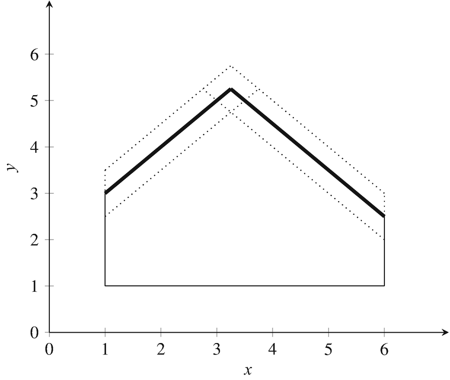
The bold line depicts the graph of Ψ(⋅ , (0, 0)), while the dotted lines correspond to the graphs of Ψ(⋅ , (±0.5, ±0.5)) and Ψ(⋅ , (∓0.5, ±0.5))

17.2.3 Continuity and Differentiability

Continuity properties of $\mathcal {R}$ carry over to Lipschitzian properties of $\mathcal {Q}_{\mathcal {R}}: P_Z \to \mathbb {R}$ , $\mathcal {Q}_{\mathcal {R}}(x) := \mathcal {R}[F(x)]$ .

Proposition 17.2.8

Assume dom f ≠ ∅ and $\mu _Z \in \mathcal {M}^p_s$ for some p ∈ [1, ∞]. Then the following statements hold true for any $\mathcal {R}: L^p(\Omega , \mathcal {F}, \mathbb {P}) \to \mathbb {R}:$

a.
$\mathcal {Q}_{\mathcal {R}}$ is locally Lipschitz continuous if $\mathcal {R}$ is convex and continuous.
b.
$\mathcal {Q}_{\mathcal {R}}$ is locally Lipschitz continuous if $\mathcal {R}$ is convex and nondecreasing.
c.
$\mathcal {Q}_{\mathcal {R}}$ is locally Lipschitz continuous if $\mathcal {R}$ is a convex risk measure .
d.
$\mathcal {Q}_{\mathcal {R}}$ is Lipschitz continuous if $\mathcal {R}$ is Lipschitz continuous.
e.
$\mathcal {Q}_{\mathcal {R}}$ is Lipschitz continuous if $\mathcal {R}$ is a coherent risk measure.△

Proof

a.
It is well-known that any real-valued convex and continuous mapping on a normed space is locally Lipschitz continuous (cf. [26]). The result is thus an immediate consequence of Lemma 17.2.4.
b.
Any real-valued, convex and nondecreasing functional on the Banach lattice $L^p(\Omega , \mathcal {F}, \mathbb {P})$ is continuous (see e.g. [27, Theorem 4.1]).
c.
By definition, any convex risk measure is convex and nondecreasing.
d.
This is a straightforward conclusion from Lemma 17.2.4.
e.
Any coherent risk measure on $L^p(\Omega , \mathcal {F}, \mathbb {P})$ is Lipschitz continuous by Inoue [28, Lemma 2.1].

□

Remark 17.2.9

Any coherent risk measure $\mathcal {R}: L^\infty (\Omega , \mathcal {F}, \mathbb {P}) \to \mathbb {R}$ is Lipschitz continuous with constant 1 by Föllmer and Schied [21, Lemma 4.3]. Concrete Lipschitz constants for continuous coherent law-invariant risk measures $\mathcal {R}: L^p (\Omega , \mathcal {F}, \mathbb {P}) \to \mathbb {R}$ with p ∈ [1, ∞) may be obtained from representation results (see e.g. [29]). △

Proposition 17.2.8 allows to formulate sufficient conditions for the existence of optimal solutions to the bilevel stochastic linear program (17.2.1):

Corollary 17.2.10

Assume dom f ≠ ∅, $\mu _Z \in \mathcal {M}^p_s$ for some p ∈ [1, ∞] and let X ⊆ P _Zbe nonempty and compact. Then (17.2.1) is solvable for any convex and nondecreasing mapping $\mathcal {R}: L^p(\Omega , \mathcal {F}, \mathbb {P}) \to \mathbb {R}$ . △

Due to the lack of convexity, Proposition 17.2.8 and the subsequent Corollary do not apply to the excess probability and the Value-at-Risk. However, invoking Lemma 17.2.1, the arguments used in the proof of [30, Proposition 3.3] can adapted to the setting of bilevel stochastic linear programming:

Proposition 17.2.11

Assume dom f ≠ ∅ and fix $\eta \in \mathbb {R}$ , then $\mathcal {Q}_{\mathit{\mbox{EP}}_\eta }$ is lower semicontinuous on P _Zand continuous at any x ∈ P _Zsatisfying

$\displaystyle \begin{aligned}\mu_Z[\lbrace z \in \mathbb{R} \; | \; f(x,z) = \eta \rbrace] = 0. \end{aligned}$

Furthermore, let X ⊆ P _Zbe nonempty and compact. Then

$\displaystyle \begin{aligned}\min_x \left\{ \mathit{\mbox{EP}}_\eta [F(x)] \; | \; x \in X \right\} \end{aligned}$

is solvable.△

$\mathcal {Q}_{\mbox{VaR}_\alpha }$ has been analyzed in [17, Theorem 2]:

Proposition 17.2.12

Assume dom f ≠ ∅ and α ∈ (0, 1), then $\mathcal {Q}_{\mathit{\mbox{VaR}}_\alpha }$ is continuous. Moreover, let X ⊆ P _Zbe nonempty and compact. Then

$\displaystyle \begin{aligned}\min_x \left\{\mathit{\mbox{VaR}}_\alpha[F(x)] \; | \; x \in X \right\} \end{aligned}$

is solvable.△

For specific risk measures, sufficient conditions for differentiability of $\mathcal {Q}_{\mathcal {R}}$ have been investigated in [31].

Proposition 17.2.13

Assume dom f ≠ ∅ and that $\mu _Z \in \mathcal {M}^1_s$ is absolutely continuous with respect to the Lebesgue measure. Fix any $\eta \in \mathbb {R}$ , then $\mathcal {Q}_{\mathbb {E}}$ and $\mathcal {Q}_{\mathit{\mbox{EE}}_\eta ^1}$ are continuously differentiable at any x ₀ ∈int P _Z. Furthermore, for any ρ ∈ [0, 1), $\mathcal {Q}_{\mathit{\mbox{SD}}_\rho ^1}$ is continuously differentiable at any x ₀ ∈int P _Zsatisfying $\mathcal {Q}_{\mathbb {E}}(x_0) \neq 0$ . △

Remark 17.2.14

Theorems 3.7, 3.8 and 3.9 in [31] provide more involved sufficient conditions for continuous differentiability of $\mathcal {Q}_{\mathbb {E}}$ , $\mathcal {Q}_{\mbox{EE}_\eta ^1}$ and $\mathcal {Q}_{\mbox{SD}_\rho ^1}$ that do not require μ _Z to be absolutely continuous.△

Remark 17.2.15

Note that the assumptions of Proposition 17.2.13 are not fulfilled in the example at the end of Sect. 17.2.2: The right-hand side of the restriction system is only partially random as the right-hand side of the restriction y ≥ 1 does not depend on Z. If we extend the system to

$\displaystyle \begin{aligned}y \leq x + 2 + z_1^{\prime}, \; y \leq -x + 8.5 + z_2^{\prime}, \; y \geq 1 + z_3^{\prime}, \end{aligned}$

the third component of the extended random vector Z′ has to take the value 0 with probability 1. Thus, $\mathbb {P} \circ Z^{\prime -1}$ is not absolutely continuous with respect to the Lebesgue measure. △

In the presence of differentiability, necessary optimality conditions for (17.2.1) can be formulated in terms of directional derivatives (cf. [31, Corollary 3.10]).

Proposition 17.2.16

Assume dom f ≠ ∅, $\mu _Z \in \mathcal {M}^p_s$ and X ⊆ P _Z. Furthermore, let x ₀ ∈ X be a local minimizer of problem (17.2.1) and assume that $\mathcal {Q}_{\mathcal {R}}$ is differentiable at x ₀. Then

$\displaystyle \begin{aligned}\mathcal{Q}^{\prime}_{\mathcal{R}}(x_0)v \geq 0 \end{aligned}$

holds for any feasible direction

$\displaystyle \begin{aligned}v \in \lbrace v \in \mathbb{R}^n \; | \; \exists \epsilon_0 > 0: \; x_0 + \epsilon v \in X \; \forall \epsilon \in [0,\epsilon_0] \rbrace. \end{aligned}$

△

17.2.4 Stability

While we have only considered $\mathcal {Q}_{\mathcal {R}}$ as a functions of the leader’s decision x so far, it also depends on the underlying probability measure μ _Z. In stochastic programming, incomplete information about the true underlying distribution or the need for computational efficiency may lead to optimization models that employ an approximation of μ _Z. This section analysis deals with the behaviour of optimal values and (local) optimal solution sets of (17.2.1) under perturbations of the underlying distribution.

Taking into account that the support of the perturbed measure may differ from the original support, we shall assume dom f ≠ ∅ and

$\displaystyle \begin{aligned}P = \mathbb{R}^n \times \mathbb{R}^s \end{aligned}$

to ensure that the objective function of (17.2.1) remains well defined. The corresponding assumption in two-stage stochastic programming is called complete recourse (cf. [1, Sect. 2.1.3]). Sufficient conditions for dom f ≠ ∅ and $P = \mathbb {R}^n \times \mathbb {R}^s$ are given in [17, Corollary 1] and [17, Corollary 2]. The following characterization is a direct consequence of Gordan’s Lemma (cf. [32]):

Lemma 17.2.17

$P = \mathbb {R}^n \times \mathbb {R}^s$ holds if and only if u = 0 is the only non-negative solution to A ^⊤u = 0. △

Throughout this section, we shall consider the situation that $\mathcal {R}: L^p(\Omega , \mathcal {F}, \mathbb {P}) \to \mathbb {R}$ with p ∈ [1, ∞) is law-invariant, convex and nondecreasing. Furthermore, for the sake of notational simplicity (cf. [31, Remark 4.1]), we assume that the probability space $(\Omega , \mathcal {F}, \mathbb {P})$ is atomless, i.e. for any $A \in \mathcal {F}$ with $\mathbb {P}[A] > 0$ there exists some $B \in \mathcal {F}$ with $B \subsetneq A$ and $\mathbb {P}[A] > \mathbb {P}[B] > 0$ .

Then for any x ∈ X and $\mu \in \mathcal {M}^p_s$ , we have $(\delta _x \otimes \mu ) \circ f^{-1} \in \mathcal {M}^p_1$ , where $\delta _x \in \mathcal {P}(\mathbb {R}^n)$ denotes the Dirac measure at x. The atomlessness of $(\Omega , \mathcal {F}, \mathbb {P})$ ensures that there exists some $Y_{(x,\mu )} \in L^p(\Omega , \mathcal {F}, \mathbb {P})$ such that $\mathbb {P} \circ Y_{(x,\mu )}^{-1} = (\delta _x \otimes \mu ) \circ f^{-1}$ . Thus, we may consider the mapping $\mathcal {Q}_{\mathcal {R}}: X \times \mathcal {M}^p_s \to \mathbb {R}$ defined by

$\displaystyle \begin{aligned}\mathcal{Q}_{\mathcal{R}}(x,\mu) := \mathcal{R}[Y_{(x,\mu)}]. \end{aligned}$

Note that the specific choice of Y _(x,μ) does not matter due to the law-invariance of $\mathcal {R}$ .

Consider the parametric optimization problem

$\displaystyle \begin{aligned} \min_x \lbrace \mathcal{Q}_{\mathcal{R}}(x,\mu) \; | \; x \in X \rbrace. \end{aligned}$

(P μ )

As (P_μ ) may be non-convex, we shall pay special attention to sets of locally optimal solutions. For any open set $V \subseteq \mathbb {R}^n$ we introduce the localized optimal value function $\varphi _V: \mathcal {M}^p_s \to \overline {\mathbb {R}}$ ,

$\displaystyle \begin{aligned}\varphi_V(\mu) := \min_x \lbrace \mathcal{Q}_{\mathcal{R}}(x,\mu) \; | \; x \in X \cap \mbox{cl} \; V \rbrace, \end{aligned}$

as well as the localized optimal solution set mapping $\phi _V: \mathcal {M}^p_s \rightrightarrows \mathbb {R}^n$ ,

$\displaystyle \begin{aligned}\phi_V(\mu) := \underset{x}{\mbox{Argmin}} \lbrace \mathcal{Q}_{\mathcal{R}}(x,\mu) \; | \; x \in X \cap \mbox{cl} \; V \rbrace. \end{aligned}$

It is well known that additional assumptions are needed when studying stability of local solutions.

Definition 17.2.18

Given $\mu \in \mathcal {M}^p_s$ and an open set $V \subseteq \mathbb {R}^n$ , ϕ _V(μ) is called a complete local minimizing (CLM) set of (P_μ ) w.r.t. V if ∅ ≠ ϕ _V(μ) ⊆ V . △

Remark 17.2.19

The set of global optimal solutions $\phi _{\mathbb {R}^n}(\mu )$ and any set of isolated minimizers are CLM sets. However, sets of strict local minimizers may fail to be CLM sets (cf. [33]). △

In the following, we shall equip $\mathcal {P}(\mathbb {R}^s)$ with the topology of weak convergence , i.e. the topology, where a sequence $\{\mu _l\}_{l \in \mathbb {N}} \subset \mathcal {P}(\mathbb {R}^s)$ converges weakly to $\mu \in \mathcal {P}(\mathbb {R}^s)$ , written ../images/480569_1_En_17_Chapter/480569_1_En_17_IEq128_HTML.gif

../images/480569_1_En_17_Chapter/480569_1_En_17_IEq128_HTML.gif

, if and only if

$\displaystyle \begin{aligned} \lim_{l \to \infty} \int_{\mathbb{R}^s} h(t)~\mu_l(dt) = \int_{\mathbb{R}^s} h(t)~\mu(dt) \end{aligned}$

holds for any bounded continuous function $h:\mathbb {R}^s \to \mathbb {R}$ (cf. [34]). The example below (cf. [22, Example 3.2]) shows that even $\varphi _{\mathbb {R}^n}$ may fail to be weakly continuous on the entire space $\mathcal {P}(\mathbb {R}^s)$ .

Example

The problem

$\displaystyle \begin{aligned}\min_x \left\{x + \int_{\mathbb{R}} z~\mu(dz) \; | \; 0 \leq x \leq 1 \right\} \end{aligned}$

arises from a bilevel stochastic linear problem, where $\mathcal {R} = \mathbb {E}$ and $\Psi (x,z) = \{z\} \subsetneq \mathbb {R}$ holds for any (x, z). Assume that μ is the Dirac measure at 0, then the above problem can be rewritten as

$\displaystyle \begin{aligned}\min_x \{x \; | \; 0 \leq x \leq 1\} \end{aligned}$

and its optimal value is 0.

However, while the sequence $\mu _l := (1 - \frac {1}{l}) \delta _{0} + \frac {1}{l} \delta _l$ converges weakly to δ ₀, replacing μ with μ _l yields the problem

$\displaystyle \begin{aligned}\min_x \left\{x + 1 \; | \; 0 \leq x \leq 1 \right\}, \end{aligned}$

whose optimal value is equal to 1 for any $l \in \mathbb {N}$ .

We shall follow the approach of [22, 31] and [35] and confine the stability analysis to locally uniformly ∥⋅∥^p-integrating sets.

Definition 17.2.20

A set $\mathcal {M} \subseteq \mathcal {M}^p_s$ is said to be locally uniformly ∥⋅∥^p-integrating if for any 𝜖 > 0 there exists some open neighborhood $\mathcal {N}$ of μ w.r.t. the topology of weak convergence such that

$\displaystyle \begin{aligned}\lim_{a \to \infty} \sup_{\nu \in \mathcal{M} \cap \mathcal{N}} \int_{\mathbb{R}^s \setminus a \mathbb{B}} \|z\|{}^p~\nu(dz) \leq \epsilon. \end{aligned}$

△

A detailed discussion of locally uniformly ∥⋅∥^p-integrating sets and their generalizations is provided in [21, 36, 37], and [38]. The following examples demonstrate the relevance of the concept.

Examples

(a)
Fix κ, 𝜖 > 0. Then by Föllmer and Schied [21, Corollary A.47 (c)], the set
$\displaystyle \begin{aligned}\mathcal{M}(\kappa, \epsilon) := \left\{ \mu \in \mathcal{P}(\mathbb{R}^s) \; | \; \int_{\mathbb{R}^s} \|z\|{}^{p + \epsilon}~\mu(dz) \leq \kappa \right\} \end{aligned}$

of Borel probability measures with uniformly bounded moments of order p + 𝜖 is locally uniformly ∥⋅∥^p-integrating.
(b)
Fix any compact set $\Xi \subset \mathbb {R}^s$ . By Föllmer and Schied [21, Corollary A.47, (b)], the set
$\displaystyle \begin{aligned}\{\mu \in \mathcal{P}(\mathbb{R}^s) \; | \; \mu[\Xi] = 1\} \end{aligned}$

of Borel probability measures whose support is contained in Ξ is locally uniformly ∥⋅∥^p-integrating.

The following result has been established in [31, Theorem 4.7]:

Theorem 17.2.21

Assume dom f ≠ ∅ and $P = \mathbb {R}^n \times \mathbb {R}^s$ . Let $\mathcal {M} \subseteq \mathcal {M}^{p}_{s}$ be locally uniformly ∥⋅∥^p-integrating, then

a.
$\mathcal {Q}_{\mathcal {R}}|{ }_{\mathbb {R}^n \times \mathcal {M}}$ is real-valued and weakly continuous.
b.
$\varphi _{\mathbb {R}^n}|{ }_{\mathcal {M}}$ is weakly upper semicontinuous.

In addition, assume that $\mu _0 \in \mathcal {M}$ is such that ϕ _V(μ ₀) is a CLM set of $P_{\mu _0}$ w.r.t. some open bounded set $V \subsetneq \mathbb {R}^n$ . Then the following statements hold true:

c.
$\varphi _V|{ }_{\mathcal {M}}$ is weakly continuous at μ ₀.
d.
$\phi _V|{ }_{\mathcal {M}}$ is weakly upper semicontinuous at μ ₀in the sense of Berge (cf. [ 39]), i.e. for any open set $\mathcal {O} \subseteq \mathbb {R}^{n}$ with $\phi |{ }_V(\mu _0) \subseteq \mathcal {O}$ there exists a weakly open neighborhood $\mathcal {N}$ of μ ₀such that $\phi _V(\mu ) \subseteq \mathcal {O}$ for all $\mu \in \mathcal {N} \cap \mathcal {M}$ .
e.
There exists some weakly open neighborhood $\mathcal {U}$ of μ ₀such that ϕ _V(μ) is a CLM set for (P_μ ) w.r.t. V for any $\mu \in \mathcal {U} \cap \mathcal {M}$ . △

Proof

Fix any $x_0 \in \mathbb {R}^n$ . By Lemma 17.2.1, f is Lipschitz continuous on $\mathbb {R}^n \times \mathbb {R}^s$ . Thus, there exists a constant L > 0 such that

$\displaystyle \begin{aligned} |f(x,z)| \leq L \|z\| + L\|x-x_0\| + |f(x_0, 0)| \end{aligned}$

and the result follows from [35, Corollary 2.4.]. □

Remark 17.2.22

Under the assumptions of Theorem 17.2.21d., any accumulation point x of a sequence local optimal solutions x _l ∈ ϕ _V(μ _l) as ../images/480569_1_En_17_Chapter/480569_1_En_17_IEq157_HTML.gif , $\mu _l \in \mathcal {M}$ , is a local optimal solution of (P_μ ). A detailed discussion of Berge’s notion of upper semicontinuity and related concepts is provided in [40, Chap. 5].△

As any Borel probability measure is the weak limit of a sequence of measures having finite support, Theorem 17.2.21 justifies an approach where the true underlying measure is approximated by a sequence of finite discrete ones. It is well known that approximation schemes based on discretization via empirical estimation [41, 42] or conditional expectations [43, 44] produce weakly converging sequences of discrete probability measures under mild assumptions.

Remark 17.2.23

All results of Sects. 17.2.1–17.2.4 can be easily extended to the pessimistic approach to bilevel stochastic linear programming, where f takes the form

$\displaystyle \begin{aligned}f(x,z) = c^\top x - \min_y \{- q^\top y \; | \; y \in \Psi(x,z)\} \end{aligned}$

(cf. [22, Chap. 4]).△

17.2.5 Stochastic Dominance Constraints

One possibility to model the minimization in

$\displaystyle \begin{aligned}\min \lbrace f(x,Z(\cdot)) \; | \; x \in X \rbrace \end{aligned}$

is doing it w.r.t. some risk measure that maps f(x, Z(⋅)) into the reals, as introduced in Sect. 17.2. In this section, we shall discuss an alternate approach, where a disutility function $g: \mathbb {R}^n \to \mathbb {R}$ is minimized over some subset of random variables of acceptable risk:

$\displaystyle \begin{aligned} \min_x \left\{g(x) \; | \; x \in X,\; f(x, Z(\cdot)) \in \mathcal{A}\right\}, \end{aligned}$

where $\mathcal {A} \subseteq f(X,Z) := \{f(x, Z(\cdot )) \; | \; x \in X\}$ . The following cases are of particular interest (cf. [1, pp. 90–91]) :

Examples

(a)
$\mathcal {A}$ is given by probabilistic constraints, i.e.
$\displaystyle \begin{aligned}\mathcal{A}_{\text{pc}} = \{h \in f(X,Z) \; | \; \mathbb{P}[h \leq \beta_j] \geq p_j \; \forall j= 1, \ldots, l\} \end{aligned}$

for bounds $\beta _1, \ldots , \beta _l \in \mathbb {R}$ and safety levels p ₁, …, p _l ∈ (0, 1).
(b)
$\mathcal {A}$ is given by first-order stochastic dominance constraints, i.e.
$\displaystyle \begin{aligned}\mathcal{A}_{\text{fo}} = \{h \in f(X,Z) \; | \; \mathbb{P}[h \leq \beta] \geq \mathbb{P}[b \leq \beta] \; \forall \beta \in \mathbb{R}\}, \end{aligned}$

where $b \in L^{0}(\Omega , \mathcal {F}, \mathbb {P})$ is a given benchmark variable. If b is discrete with a finite number of realizations, it is sufficient to impose the relation $\mathbb {P}[h \leq \beta ] \geq \mathbb {P}[b \leq \beta ]$ for any β in a finite subset of $\mathbb {R}$ . In this case, $\mathcal {A}$ admits a description by a finite system of probabilistic constraints.
(c)
$\mathcal {A}$ is given by second-order stochastic dominance constraints, i.e.
$\displaystyle \begin{aligned}\mathcal{A}_{\text{so}} = \{h \in f(X,Z) \; | \; \mathbb{E}[\max\{h - \eta, 0\}] \leq \mathbb{E}[\max\{b - \eta, 0\}] \; \forall \eta \in \mathbb{R}\}, \end{aligned}$

where $b \in L^{1}(\Omega , \mathcal {F}, \mathbb {P})$ is a given benchmark variable.

A discussion of general models involving probabilistic or stochastic dominance constraints can be found in [1, Chap. 8] and [45, Chap. 8.3].

Let $\nu := \mathbb {P} \circ b^{-1} \in \mathcal {P}(\mathbb {R})$ denote the distribution of the benchmark variable b. Then the feasible set under first-order stochastic dominance constraints admits the representation

$\displaystyle \begin{aligned}\left\{ x \in X \; | \; \mu_Z\big[ \lbrace z \in \mathbb{R}^s \; | \; f(x,z) \leq \beta \rbrace \big] \geq \nu\big[ \lbrace b \in \mathbb{R} \; | \; b \leq \beta \rbrace \big] \; \forall \beta \in \mathbb{R} \right\}. \end{aligned}$

Similarly, for second-order stochastic dominance constraints, $\mu \in \mathcal {M}^1_s$ and $\nu \in \mathcal {M}^1_1$ , the feasible set takes the form

$\displaystyle \begin{aligned}\left\{ x \in X \, | \int_{\mathbb{R}^s} \max \lbrace f(x,z) - \eta, 0 \rbrace~\mu_Z(dz) \leq \int_{\mathbb{R}} \max \lbrace b - \eta, 0 \rbrace~\nu(db) \; \forall \eta \in \mathbb{N} \right\}. \end{aligned}$

In both cases, the feasibility does only depend on the distribution of the underlying random vector . As in Sect. 17.2.4, we consider situations where μ _Z is replaced with an approximation and study the behaviour of the mappings $\mathcal {C}_1: \mathbb {P}(\mathbb {R}^s) \rightrightarrows \mathbb {R}^n$ defined by

$\displaystyle \begin{aligned}\mathcal{C}_1(\mu) = \left\{ x \in X \; | \; \mu \big[ \lbrace z \in \mathbb{R}^s \; | \; f(x,z) \leq \beta \rbrace \big] \geq \nu\big[ \lbrace b \in \mathbb{R} \; | \; b \leq \beta \rbrace \big] \; \forall \beta \in \mathbb{R} \right\}. \end{aligned}$

and $\mathcal {C}_2: \mathcal {M}^1_s \rightrightarrows \mathbb {R}^n$ given by

$\displaystyle \begin{aligned}C_2(\mu) := \left\{ x \in X \, | \int_{\mathbb{R}^s} \max \lbrace f(x,z) - \eta, 0 \rbrace~\mu(dz) \leq \int_{\mathbb{R}} \max \lbrace b - \eta, 0 \rbrace~\nu(db) \, \forall \eta \in \mathbb{N} \right\}. \end{aligned}$

Invoking Lemma 17.2.1, the following result can be obtained by adapting the proofs of [46, Proposition 2.1] and [47, Proposition 2.2] :

Proposition 17.2.24

Assume dom f ≠ ∅ and $P = \mathbb {R}^n \times \mathbb {R}^s$ . Then the following statements hold true:

a.
The multifunction C ₁is closed w.r.t. the topology of weak convergence , i.e. for any sequences $\lbrace \mu _{l} \rbrace _{l} \subset \mathcal {P}(\mathbb {R}^{s})$ and $\lbrace x_{l} \rbrace _{l} \subset \mathbb {R}^{n}$ with , $x_{l} \rightarrow x \in \mathbb {R}^{n}$ for l →∞ and x _l ∈ C ₁(μ _l) for all $l \in \mathbb {N}$ it holds true that x ∈ C ₁(μ).
b.
Additionally assume that $\nu \in \mathcal {M}^1_1$ , then the multifunction C ₂is closed w.r.t. the topology of weak convergence.△

By considering the constant sequence μ _l = μ for all $l \in \mathbb {N}$ we obtain the closedness of the sets C ₁(μ) and C ₂(μ) under the conditions of Proposition 17.2.24. The closedness of the multifunctions C ₁ and C ₂ is also the key to proving the following stability result (cf. [46, Proposition 2.5]):

Theorem 17.2.25

Assume dom f ≠ ∅, $P = \mathbb {R}^n \times \mathbb {R}^s$ and that X is nonempty and compact. Moreover, let g be lower semicontinuous. Then the following statements hold true:

a.
The optimal value function $\varphi _1: \mathcal {P}(\mathbb {R}^{s}) \to \mathbb {R} \cup \lbrace \infty \rbrace$ given by
$\displaystyle \begin{aligned}\varphi_1(\mu) := \inf \lbrace g(x) \; | \; x \in C_1(\mu)\rbrace \end{aligned}$

is weakly lower semicontinuous on dom C ₁.
b.
Additionally assume $\nu \in \mathcal {M}^1_1$ , then the function $\varphi _2: \mathcal {M}^1_s \to \mathbb {R} \cup \lbrace \infty \rbrace$ given by
$\displaystyle \begin{aligned}\varphi_2(\mu) := \inf \lbrace g(x) \; | \; x \in C_2(\mu)\rbrace \end{aligned}$

is weakly lower semicontinuous on dom C ₂. △

17.2.6 Finite Discrete Distributions

Throughout this section, we shall assume that the underlying random vector Z is discrete with a finite number of realizations $Z_1, \ldots , Z_K \in \mathbb {R}^s$ and respective probabilities π ₁, …, π _K ∈ (0, 1]. Let I denote the index set {1, …, K}, then P _Z takes the form

$\displaystyle \begin{aligned}P_Z = \lbrace x \in \mathbb{R}^n \; | \; \forall k \in I \; \exists y \in \mathbb{R}^m: \; Ay \leq Tx + Z_k \rbrace. \end{aligned}$

Suppose that x ₀ ∈ X is such that $\lbrace y \in \mathbb {R}^m \; | \; Ay \leq Tx_0 + Z_k \rbrace = \emptyset$ holds for some k ∈ I. Then the probability of f(x ₀, Z(ω)) = ∞ is a least π _k > 0, i.e. x ₀ should be considered as infeasible for problem (17.2.1). Consequently, X ⊆ P _Z can be understood as an induced constraint. Note that X ∩ P _Z is a polyhedron if X is a polyhedron.

In this setting, the bilevel stochastic linear problem can be reduced to a standard bilevel program, which allows to adapt optimality conditions and algorithms designed for the deterministic case (cf. [48]).

Proposition 17.2.26

Assume

../images/480569_1_En_17_Chapter/480569_1_En_17_IEq189_HTML.gif

../images/480569_1_En_17_Chapter/480569_1_En_17_IEq190_HTML.gif

$\mathcal {R}_{\max } \rbrace$ and let X ⊆ P _Zbe a polyhedron. If $\mathcal {R} \in \lbrace \mathit{\mbox{EP}}_{\eta }, \mathit{\mbox{VaR}}_{\alpha } \rbrace$ , additionally assume that X bounded. Then for any parameter β, there exists a constant M > 0 such that the bilevel stochastic linear problem

$\displaystyle \begin{aligned}\min_x \left\{ \mathcal{R}[F(x)] \; | \; x \in X \right\} \end{aligned}$

is equivalent to the standard bilevel program

$\displaystyle \begin{aligned}\min_x \Big\{\underbrace{\ \;\inf_{\eta \in \mathbb{R}}}_{\mathit{\text{if}}\ \mathcal{R} = \mathit{\mbox{CVaR}}_{\alpha}}\ \min_w \big\{a(x, w) \; | \; w \in \Psi_{\mathcal{R}}(x)\big\}| \; x \in X\Big\},\ \mathit{\text{or}} \end{aligned}$

$\displaystyle \begin{aligned}\min_x \Big\{c^\top x + \inf_{\eta \in \mathbb{R}}\big\{\eta \; | \; \min_w \{a(x, w) \; | \; w \in \Psi_{\mathcal{R}}(x)\} \geq \alpha\big\}| \; x \in X\Big\}\quad \mathit{\text{if}}\ \mathcal{R}= \mathit{\mbox{VaR}}_{\alpha}, \end{aligned}$

where $\Psi _{\mathcal {R}}: \mathbb {R}^n \rightrightarrows \mathbb {R}^{\mathit{\mbox{dim}}\;w}$ with

$\displaystyle \begin{aligned}\Psi_{\mathcal{R}}(x) := \underset{w}{\mathit{\mbox{Argmin}}} \; \left\{\sum_{k \in I}d^\top y_k \; | \; Ay_k \leq Tx + Z_k,\;b_k(x, w) \geq 0\ \forall k \in I\right\}. \end{aligned}$

The specific formulations can be found in Table 17.1. △

Table 17.1

Equivalent bilevel linear programs

$\mathcal {R}$	β	w	a(x, w)	b(x, w)
$\mathbb {E}$		$(y_1, \ldots , y_K) \in \mathbb {R}^{Km}$	c ^⊤x+∑_{k ∈ I}π _kq ^⊤y _k
$\mbox{EE}^1_{\eta }$	$\eta \in \mathbb {R}$	$\begin {array}{l} (y_1, \ldots , y_K) \in \mathbb {R}^{Km} \\ (v_1, \ldots , v_K) \in \mathbb {R}^{K}\end {array}$	∑_{k ∈ I}π _kv _k	$\left (\begin {array}{l}v_k\\v_k - c^\top x - q^\top y_k {+} \eta \end {array}\right )$
$\mbox{SD}^1_\rho$	ρ ∈ (0, 1]	$\begin {array}{l} (y_1, \ldots , y_K) \in \mathbb {R}^{Km} \\ (v_1, \ldots , v_K) \in \mathbb {R}^{K}\end {array}$	$\begin {array}{l}(1 - \rho )\sum _{k \in I}\pi _k q^\top y_k\\ + \rho \sum _{k \in I}\pi _k v_k + c^\top x\end {array}$	$\left (\begin {array}{l}v_k - q^\top y_k\\v_k - \sum _{j \in I}\pi _j q^\top y_j\end {array}\right )$
EP_η	$\eta \in \mathbb {R}$	$\begin {array}{l} (y_1, \ldots , y_K) \in \mathbb {R}^{Km} \\ (\theta _1, \ldots , \theta _K) \in \lbrace 0,1 \rbrace ^{K}\end {array}$	∑_{k ∈ I}π _kθ _k	Mθ _k−c ^⊤x−q ^⊤y _k+η
VaR_α	α ∈ (0, 1)	$\begin {array}{l} (y_1, \ldots , y_K) \in \mathbb {R}^{Km} \\ (\theta _1, \ldots , \theta _K) \in \lbrace 0,1 \rbrace ^{K}\end {array}$	∑_{k ∈ I}π _kθ _k	$\begin {array}{l}M(1 - \theta _k) - c^\top x\\ - q^\top y_k + \eta \end {array}$
CVaR_α	α ∈ (0, 1)	$\begin {array}{l} (y_1, \ldots , y_K) \in \mathbb {R}^{Km} \\ (v_1, \ldots , v_K) \in \mathbb {R}^{K}\end {array}$	$\eta + \frac {1}{1 - \alpha }\sum _{k \in I}\pi _k v_k$	cf. $\mbox{EE}^1_{\eta }$
$\mathcal {R}_{\max }$		$(y_1, \ldots , y_K) \in \mathbb {R}^{Km}$	max_{k ∈ I}c ^⊤x+q ^⊤y _k

Proof

For $\mathcal {R} \in \lbrace \mathbb {E}, \mbox{EE}_\eta ^1, \mbox{SD}^1_\rho , \mbox{CVaR}_\alpha \rbrace$ , we refer to [31, Section 5].

For the excess probability, the first of the considered quantile-based risk measures, we have $\mbox{EP}_{\eta }[F(x)] = \mathbb {P}\left [c^\top x + \inf _y \{q^\top y \; | \; y \in \Psi (x, Z(\cdot ))\} > \eta \right ]$ . Fix $M \in \mathbb {R}$ such that

$\displaystyle \begin{aligned} M > \sup\big\{c^\top x + \inf_{y_k} \big\{q^\top y_k \; | \; y_k \in \Psi(x, Z_k)\big\} \; | \; x \in X,\; k \in I\big\} - \eta\end{aligned}$

and, for y _k ∈ Ψ(x, Z _k), let

$\displaystyle \begin{aligned} \theta_k := \begin{cases} 0 & \text{if}\ c^\top x + q^\top y_k - \eta \leq 0,\\ 1 & \text{otherwise.} \end{cases} \end{aligned}$

Then the excess probability is equal to

$\displaystyle \begin{aligned} \begin{array}{rcl} &\displaystyle \sum_{k \in I}\pi_k \inf_{y_k, \theta_k} \left\{\theta_k \; | \; M\theta_k \geq c^\top x + q^\top y_k - \eta,\; y_k \in \Psi(x, Z_k),\; \theta_k \in \{0, 1\}\right\}\\ &\displaystyle \left. \begin{aligned} = \inf_{\genfrac{}{}{0pt}{}{y_1, \ldots, y_K,}{\theta_1, \ldots, \theta_K}} \left\{\sum_{k \in I}\pi_k \theta_k \; | \; \right.&\displaystyle M\theta_k \geq c^\top x + q^\top y_k - \eta,\; y_k \in \Psi(x, Z_k),\; \theta_k \in \{0, 1\}\\ &\displaystyle \forall k \in I \end{aligned} \right\}. \end{array} \end{aligned}$

Similar to the proof for $\mathcal {R} = \mbox{EP}_\eta$ , the expression $\mathbb {P}[f(x,Z(\cdot )) \leq \eta ]$ equals

$\displaystyle \begin{aligned} &\sum_{k \in I}\pi_k \inf_{y_k, \theta_k} \left\{\theta_k \; | \; M(1 - \theta_k) \geq c^\top x + q^\top y_k - \eta,\; y_k \in \Psi(x, Z_k),\; \theta_k \in \{0, 1\} \right\}\\ &\left. \begin{aligned} = \left.\inf_{\genfrac{}{}{0pt}{}{y_1, \ldots, y_K,}{\theta_1, \ldots, \theta_K}} \right\{\sum_{k \in I}\pi_k \theta_k \; | \; &M(1 - \theta_i) \geq c^\top x + q^\top y_k - \eta,\; y_k \in \Psi(x, Z_k),\; \theta_k \in \{0, 1\} \\ &\forall k \in I \end{aligned} \right\}, \end{aligned}$

where

$\displaystyle \begin{aligned}\theta_k := \begin{cases} 1 & \text{if}\ c^\top x + q^\top y_k - \eta \leq 0,\\ 0 & \text{otherwise.} \end{cases} \end{aligned}$

Thereby we get equality of VaR_η[f(x, Z(⋅))] and

$\displaystyle \begin{aligned} \inf \left\{\eta \in \mathbb{R} \; | \; \inf_{\genfrac{}{}{0pt}{}{y_1, \ldots, y_K,}{\theta_1, \ldots, \theta_K}} \left\{\sum_{k \in I}\pi_k \theta_k \; | \; (y_1, \ldots, y_K, \theta_1, \ldots, \theta_K) \in \Psi_{\mbox{VaR}_{\eta}}(x) \right\} \geq \alpha\right\}. \end{aligned}$

The worst-case risk measure is equal to $\sup _{k \in I} \left \{c^\top x + \min _{y_k} \{q^\top y \; | \; y {\in } \Psi (x, Z_k)\}\right \}$ and the result follows from $\Psi _{\mathcal {R}_{\max }} = \Psi (x, Z_1) \times \ldots \times \Psi (x, Z_K)$ . □

Remark 17.2.27

a.
The equivalent standard bilevel problem is linear provided that $\mathcal {R} \in \lbrace \mathbb {E}, \mbox{EE}_\eta ^1, \mbox{SD}_{\rho }^1 \rbrace$ .
b.
Analogous to [31, Remarks 5.2, 5.4], the inner minimization problems of the standard bilevel linear programs for $\mathcal {R} \in \lbrace \mathbb {E}, \mbox{EE}_\eta ^1, \mbox{EP}_\eta , \mathcal {R}_{\max } \rbrace$ can be decomposed into K scenario problems that only differ w.r.t. the right-hand side of the constraint system. For the other models, a similar decomposition is possible after Lagrangian relaxation of the coupling constraints involving different scenarios.
c.
For $\mathcal {R} = \mbox{CVaR}_\alpha$ , every evaluation of the objective function in the standard bilevel linear program corresponds to solving a bilevel linear problem with scalar upper level variable η.
d.
Alternate models for $\mathcal {R} = \mbox{VaR}_\alpha$ are given in [17] and [49], where the considered bilevel stochastic linear problem is reduced to a mixed-integer nonlinear program and a mathematical programming problem with equilibrium constraints, respectively. A mean-risk model with $\mathcal {R} = \mbox{CVaR}_\alpha$ is used in [5, Sect. III].△

Similar reformulations can be obtained for the models discussed in Sect. 17.2.5 if we assume that the disutility function is linear.

Proposition 17.2.28

Assume dom f ≠ ∅, and let X ⊆ P _Zbe a bounded polyhedron. Then for any parameter γ, the problem

$\displaystyle \begin{aligned} \min_x \left\{g^\top x \; | \; F(x) \in \mathcal{A},\; x \in X \right\} \end{aligned}$

is equivalent to

$\displaystyle \begin{aligned} \min_x \Big\{g^\top x \; | \; \inf_{w_j} \left\{a(w_j) \; |\; w_j \in \Psi_{\mathcal{R}}(x)\right\} \geq \delta_j \ \forall j = 1, \ldots, l,\; x \in X\Big\}. \end{aligned}$

The specific formulations are listed in Table 17.2, where $\bar {a}_j := 1 - \mathbb {P}[b \leq a_j]$ and $\tilde {a}_j := \int _{\mathbb {R}^s}\max \{b(z) - a_j, 0\}\;\mu _Z(dz)$ .

Table 17.2

Equivalent programs, notation as in the Example in Sect. 17.2.5

$\mathcal {A}$	γ	w _j	a(w _j)	$\mathcal {R}$	δ _j
$\mathcal {A}_{\text{pc}}$	$\begin {array}{l}\beta _j \in \mathbb {R},\ p_j \in (0, 1)\\\text{with}\ j = 1, \ldots , l\end {array}$	$\begin {array}{l} (y_{1j}, \ldots , y_{Kj}) \in \mathbb {R}^{Km} \\ (\theta _{1j}, \ldots , \theta _{Kj}) \in \lbrace 0,1 \rbrace ^{K}\end {array}$	∑_{k ∈ I}π _kθ _kj	$\mbox{VaR}_{\beta _j}$	p _j
$\mathcal {A}_{\text{fo}}$	$\begin {array}{l}\text{any finite discrete}\\\text{benchmark variable}\end {array}$	$\begin {array}{l} (y_{1j}, \ldots , y_{Kj}) \in \mathbb {R}^{Km} \\ (\theta _{1j}, \ldots , \theta _{Kj}) \in \lbrace 0,1 \rbrace ^{K}\end {array}$	∑_{k ∈ I}π _kθ _kj	$\mbox{EP}_{a_j}$	$\bar {a}_j$
$\mathcal {A}_{\text{so}}$	$\begin {array}{l}b\ \text{with realizations}\\a_1, \ldots , a_l\end {array}$	$\begin {array}{l} (y_{1j}, \ldots , y_{Kj}) \in \mathbb {R}^{Km} \\ (v_{1j}, \ldots , v_{Kj}) \in \mathbb {R}^{K}\end {array}$	∑_{k ∈ I}π _kv _kj	$\mbox{EE}_{a_j}^1$	$\tilde {a}_j$

△

17.2.7 Solution Approaches

To solve bilevel problems, it is very common to use a single level reformulation. Often the lower level minimality condition is replaced by its Karush-Kuhn-Tucker or Fritz John conditions and the bilevel problem is reduced to a mathematical programming problem with equilibrium constraints (cf. [5, 17], [48, Chap. 3.5.1]).

For $\mathcal {R} \in \lbrace \mathbb {E}, \mbox{EE}_\eta ^1, \mbox{SD}^1_\rho , \mbox{EP}_\eta , \mathcal {R}_{\max } \rbrace$ , the equivalent standard bilevel programs in Proposition 17.2.26 can be all restated as

$\displaystyle \begin{aligned} \min_u \big\{g^\top u + \min_w \lbrace h^\top w \; | \; w \in \Psi(u) \rbrace \; | \; u \in U\big\}, \end{aligned}$

(17.2.2)

where $\Psi : \mathbb {R}^k \rightrightarrows \mathbb {R}^l$ is given by Ψ(u) = Argmin_w{t ^⊤w | Ww ≤ Bu + b} for vectors $g \in \mathbb {R}^k$ , $h, t \in \mathbb {R}^l$ and $b \in \mathbb {R}^r$ , matrices $W \in \mathbb {R}^{r \times l}$ and $B \in \mathbb {R}^{r \times k}$ , and $U \subseteq \mathbb {R}^k$ is a nonempty polyhedron. The usage of the KKT conditions of the lower level problem leads to the single-level problem

$\displaystyle \begin{aligned} \min_{u, w, v} \left\{ g^\top u + h^\top w \; \Bigg| \; \begin{aligned} &Ww \leq Bu + b, \; W^\top v = t, \; v \leq 0, \\ &v^\top (Ww - Bu - b) = 0, \; u \in U \end{aligned} \right\}. \end{aligned}$

(17.2.3)

More details as well as statements on the coincidence of optimal values and the existence of local and global minimizers are given in [31, Sect. 6]. If the condition v ^⊤(Ww − Bu − b) = 0 is relaxed by v ^⊤(Ww − Bu − b) ≤ ε (the resulting problem is denoted by P(ε)), the violation of regularity conditions like (MFCQ) and (LICQ) at every feasible point of (17.2.3) can be bypassed. A discussion of other difficulties associated with (17.2.3) is provided in [11, Chap. 3.1.2].

In [31, Sect. 6] it is also shown that $(\bar {u}, \bar {w})$ is a local minimizer of the optimistic formulation, if $(\bar {u}, \bar {w}, \bar {v})$ is an accumulation point of a sequence $\lbrace (u_n, w_n, v_n) \rbrace _{n \in \mathbb {N}}$ of local minimizers of problem P(ε _n) for ε _n ↓ 0.

In the risk-neutral setting, problem (17.2.2) exhibits a block-structure (cf. Remark 17.2.27 b.). Adapting the solution method for general linear complementarity problems proposed in [50], this special structure has been used in [11, Chap. 6] to construct an efficient algorithm for the global resolution of bilevel stochastic linear problems based on dual decomposition.

Remark 17.2.29

Utilizing the lower level value function, problem (17.2.2) can be reformulated as a single level quasiconcave optimization problem (cf. [48, Chap. 3.6.5]). Solution methods based on a branch-and-bound scheme have been proposed in [51] and [52]. However, without modifications, these algorithms fail to exploit the block structure arising in risk-neutral bilevel stochastic linear optimization models (cf. [11, Chap. 4.2]). △

17.3 Two-Stage Stochastic Bilevel Programs

In two-stage stochastic bilevel programming, both leader and follower have to make their respective first-stage decisions without knowledge of the realization of a stochastic parameter. Afterwards, the second-stage decisions are made under complete information. This leads to the following chronology of decision and observation:

../images/480569_1_En_17_Chapter/480569_1_En_17_Equbs_HTML.png

Remark 17.3.1

The bilevel stochastic linear problems considered in Sect. 17.2 can be understood as special two-stage bilevel programs, where the follower’s first-stage and the leader’s second stage decision do not influence the outcome. △

In [12], a two-stage stochastic extension of the bilevel network pricing model introduced in [53] is studied. Consider a multicommodity transportation network (N, Λ, K), where (N, Θ) is a directed graph and each commodity k ∈ K is to be transported from an origin O(k) ∈ N to a destination D(k) ∈ N in order to satisfy a demand n ^k ∈ (0, ∞). The set of arcs Θ is partitioned into the subsets θ and $\bar {\theta }$ of tariff and tariff-free arcs, respectively, and the leaders is maximizing the revenue raised from tariffs, knowing that user flows are assigned to cheapest paths. In [53], this situation is modeled as a bilevel program

$\displaystyle \begin{aligned}\text{``}\max_{x}\text{''} \left\{ \sum_{k \in K} x^\top y^k \; | \; (y,\bar{y}) \in \Psi(x) \right\}, \end{aligned}$

where the lower level is given by

$\displaystyle \begin{aligned}\Psi(x, c, d, b) := \underset{y,\bar{y}}{\mbox{Argmin}} \left\{ \sum_{k \in K} \left[ (c + x)^\top y^k + \bar{c}^\top \bar{y}^k \right] \; \Big| \; \begin{array}{l} y, \bar{y} \geq 0, \\ Ay^k + \bar{A} \bar{y}^k = b^k \; \forall k \in K \end{array} \right\}, \end{aligned}$

and x is the vector of tariffs controlled by the leader, y ^k and $\bar {y}^k$ are the flows of commodity k on the tariff and tariff-free arcs, respectively. Moreover, c and $\bar {c}$ are the fixed costs on θ and $\bar {\theta }$ , respectively, $(A,\bar {A})$ denotes the node-arc incidence matrix and the vectors b ^k defined by

$\displaystyle \begin{aligned}b^k_i := \begin{cases} n^k, &\text{if} \; i = O(k) \\ -n^k, &\text{if} \; i = D(k) \\ 0, &\text{else} \end{cases} \end{aligned}$

are used to express nodal balance. Reference [12] extends the above model to a two-stage setting including market uncertainties: After deciding on first-stage tariffs, the situation repeats itself on the same network but with different cost and demand parameters. At the first-stage , only the distribution of the second-stage parameter Z(ω) = (c ₂, d ₂, b ₂)(ω) is known and the stages are linked by the restriction that the second-stage tariffs should not differ too widely from those set at the first stage. The linking constraint is motivated by policy regulations and competitivity issues. In a risk-neutral setting, this results in the problem

$\displaystyle \begin{aligned} \text{``}\max_{x_1}\text{''} \left\{ \sum_{k \in K} x_1^\top y^k_1 + \mathbb{E}[\Phi(x_1, Z(\cdot))] \; | \; (y_1,\bar{y}_1) \in \Psi(x_1,c_1,d_1,b_1) \right\}, \end{aligned}$

(17.3.1)

where the recourse is given by

$\displaystyle \begin{aligned}\Phi(x_1, Z(\omega)) := \text{``}\max_{x_2}\text{''} \left\{ \sum_{k \in K} x_2^\top y^k_2 \; | \; (x_1,x_2) \in \Gamma(\delta), \; (y_2,\bar{y}_2) \in \Psi(x_2,Z(\omega)) \right\} \end{aligned}$

and the set Γ(δ) is defined as either

$\displaystyle \begin{aligned}\Gamma(\delta) := \Gamma_A(\delta) := \lbrace (x_1,x_2) \; | \; |x_{1, \theta} - x_{2, \theta}| \leq \delta_\theta \; \forall \theta \in \Theta \rbrace \end{aligned}$

if tariff changes are limited in absolute values or

$\displaystyle \begin{aligned}\Gamma(\delta) := \Gamma_R(\delta) := \lbrace (x_1,x_2) \; | \; |x_{1, \theta} - x_{2, \theta}| \leq \delta_\theta |x_{1, \theta}| \; \forall \theta \in \Theta \rbrace \end{aligned}$

if proportional limits are considered. Assuming that the underlying random vector Z is discrete with a finite number of realizations, a reformulation of (17.3.1) as a single-stage bilevel program is established in [12]. Moreover, sensitivity analysis of the optimal value function of (17.3.1) w.r.t. the parameter δ ∈ [0, ∞)^{| Θ|} (cf. [12, Proposition 4.1, Proposition 4.2]) as well as numerical studies are conducted (cf. [12, Sects. 5, 6]).

17.4 Challenges

We shall highlight some aspects of bilevel stochastic programming that are highly deserving of future research:

Going (Further) Beyond the Risk-Neutral Case for Nonlinear Models

The first paper on bilevel stochastic programming has already outlined the basic principles as well as existence and sensitivity results for risk neutral models (cf. [2]). Nevertheless, so far, most of the research on bilevel stochastic nonlinear programming is still concerned with the risk-neutral case. Notable exceptions are [5] and [8], where models involving the Conditional Value-at-Risk are considered. In the first paper the problem of maximizing the medium-term revenue of an electricity retailer under uncertain pool prices, demand, and competitor prices is modeled as a bilevel stochastic quadratic problem, while the latter explores links between electricity swing option pricing and bilevel stochastic optimization. However, there exists no systematic analysis of bilevel stochastic nonlinear problems in the broader framework of coherent risk measures or higher stochastic dominance constraints. Future research may also consider distributionally robust models (cf. [54]).

Exploiting (Quasi) Block Structures Arising in Risk-Averse Models

Under finite discrete distributions many bilevel stochastic problems can be reformulated as standard bilevel programs. While this reformulation entails a blow-up of the dimension which is usually linear in the number of scenarios, the resulting problems often exhibit (quasi) block structures (cf. Remark 17.2.27b., [2]). For risk-neutral bilevel stochastic linear problems, [11, Chap. 6] utilizes these structures to enhance the mixed integer programming based solution algorithm of [50] resulting in a significant speed-up. Based on the structural similarities an analogous approach should be possible for risk-averse models after Lagrangian relaxation of coupling constraints.

Going Beyond Exogenous Stochasticity

While the analysis in the vast majority of papers on stochastic programming is confined to the case of purely exogenous stochasticity, this assumption is known to be unrealistic in economic models, where the decision maker holds market power. Therefore, models with decision dependent distributions are of particular interest in view of stochastic Stackelberg games (cf. [55]).

Acknowledgements

The second author thanks the Deutsche Forschungsgemeinschaft for its support via the Collaborative Research Center TRR 154.

References

1.
A. Shapiro, D. Dentcheva, A. Ruszczyński, Lectures on Stochastic Programming: Modeling and Theory. MPS SIAM Series on Optimization, vol. 9, 2nd edn. (SIAM, Philadelphia, 2014)
2.
M. Patriksson, L. Wynter, Stochastic mathematical programs with equilibrium constraints. Oper. Res. Lett. 25, 159–167 (1999)
3.
S. Christiansen, M. Patriksson, L. Wynter, Stochastic bilevel programming in structural optimization. Struct. Multidiscip. Optim. 21, 361–371 (2001)
4.
A. Werner, Bilevel stochastic programming problems: analysis and application to telecommunications. PhD thesis, Norwegian University of Science and Technology, 2005
5.
M. Carrión, J.M. Arroyo, A.J. Conejo, A bilevel stochastic programming approach for retailer futures market trading. IEEE Trans. Power Syst. 24, 1446–1456 (2009)
6.
S. Dempe, V.V. Kalashnikov, G.A. Pérez-Valdés, N.I. Kalashnykova, Natural gas bilevel cash-out problem: convergence of a penalty function method. Eur. J. Oper. Res. 215, 532–538 (2011)
7.
S. Kosuch, P. Le Bodic, J. Leung, A. Lisser, On a stochastic bilevel programming problem. Networks 59, 107–116 (2012)
8.
R.M. Kovacevic, G.C. Pflug, Electricity swing option pricing by stochastic bilevel optimization: a survey and new approaches. Eur. J. Oper. Res. 237, 389–403 (2013)
9.
A. Chen, J. Kim, Z. Zhou, P. Chootinan, Alpha reliable network design problem. Transp. Res. Rec. 2029, 49–57 (2007)
10.
M. Patriksson, On the applicability and solution of bilevel optimization models in transportation science: a study on the existence, stability and computation of optimal solutions to stochastic mathematical programs with equilibrium constraints. Transp. Res. Part B Method. 42, 843–860 (2008)
11.
C. Henkel, An algorithm for global resolution of linear stochastic bilevel programs. PhD thesis, University of Duisburg-Essen, 2014
12.
S.M. Alizadeh, P. Marcotte, G. Savard, Two-stage stochastic bilevel programming over a transportation network. Transp. Res. B 58, 92–105 (2013)
13.
B.C. Eaves, On quadratic programming. Manag. Sci. 17, 698–711 (1971)
14.
K. Beer, Lösung großer linearer Optimierungsaufgaben (Deutscher Verlag der Wiss., Berlin, 1977)
15.
D. Klatte, B. Kummer, Stability properties of infima and optimal solutions of parametric optimization problems, in Nondifferentiable Optimization: Motivations and Applications, Proceedings of the IIASA Workshop, Sopron. Lect. Notes Econ. Math. Syst., vol. 255 (Springer, Berlin, 1984), pp. 215–229
16.
D. Klatte, G. Thiere, Error bounds for solutions of linear equations and inequalities. ZOR Math. Methods Oper. Res. 41, 191–214 (1995)
17.
S.V. Ivanov, Bilevel stochastic linear programming problems with quantile criterion. Autom. Remote Control 75, 107–118 (2014)
18.
G.B. Dantzig, Linear Programming and Extensions (Princeton University Press, Princeton, 1963)
19.
P. Artzner, F. Delbaen, J.-M. Eber, D. Heath, Coherent measures of risk. Math. Financ. 9, 203–228 (1999)
20.
H. Föllmer, A. Schied, Convex measures of risk and trading constraints. Finance Stoch. 6, 429–447 (2002)
21.
H. Föllmer, A. Schied, Stochastic Finance: An Introduction in Discrete Time, 3rd edn. (de Gruyter, Berlin, 2011)
22.
M. Claus, Advancing stability analysis of mean-risk stochastic programs: bilevel and two-stage models. PhD thesis, University of Duisburg-Essen, 2016
23.
G.C. Pflug, Some remarks on the value-at-risk and the conditional value-at-risk, in Probabilistic Constrained Optimization - Methodology and Application, ed. by S.P. Uryasev (Kluwer Academic, Dordrecht, 2000), pp. 272–281
24.
R.T. Rockafellar, S. Uryasev, Conditional value-at-risk for general loss distributions. J. Bank. Financ. 26, 1443–1471 (2002)
25.
A. Ben-Tal, L. El Ghaoui, A. Nemirovski, Robust Optimization (Princeton University Press, Princeton, 2009)
26.
I. Ekeland, R. Temam, Analyse convexe et problèmes variationnels (Dunod, Paris, 1974)
27.
P. Cheridito, T. Li, Risk measures on Orlicz hearts. Math. Financ. 18, 189–214 (2009)
28.
A. Inoue, On the worst case conditional expectation. J. Math. Anal. Appl. 286, 237–247 (2003)
29.
D. Belomestny, V. Krätschmer, Central limit theorems for law-invariant coherent risk measures. J. Appl. Prob. 49, 1–21 (2012)
30.
R. Schultz, S. Tiedemann, Risk aversion via excess probabilities in stochastic programs with mixed-integer recourse. SIAM J. Optim. 14, 115–138 (2003)
31.
J. Burtscheidt, M. Claus, S. Dempe, Risk-averse models in bilevel stochastic linear programming. Preprint, arXiv:1901.11349 [math.OC] (2019)
32.
P. Gordan, Über die Auflösungen linearer Gleichungen mit reellen Coefficienten. Math. Ann. 6, 238 (1873)
33.
S.M. Robinson, Local epi-continuity and local optimization. Math. Program. 37, 208–222 (1987)
34.
P. Billingsley, Convergence of Probability Measures (Wiley, New York, 1968)
35.
M. Claus, V. Krätschmer, R. Schultz, Weak continuity of risk functionals with applications to stochastic programming. SIAM J. Optim. 27, 91–109, S108 (2017)
36.
V. Krätschmer, A. Schied, H. Zähle, Qualitative and infinitesimal robustness of tail-dependent statistical functionals. J. Multivar. Anal. 103, 35–47 (2012)
37.
V. Krätschmer, A. Schied, H. Zähle, Comparative and qualitative robustness for law-invariant risk measures. Finance Stoch. 18, 271–295 (2014)
38.
V. Krätschmer, A. Schied, H. Zähle, Domains of weak continuity of statistical functionals with a view on robust statistics. J. Multivar. Anal. 158, 1–19 (2017)
39.
C. Berge, Espaces topologiques: fonctions multivoques. Coll. Universitaire de mathématiques, vol. 3 (Dunod, Paris, 1959)
40.
R.T. Rockafellar, R.J.-B. Wets, Variational Analysis (Springer, Berlin, 2009)
41.
D. Pollard, Convergence of Stochastic Processes (Springer, New York, 1984)
42.
G.R. Shorack, J.A. Wellner, Empirical Processes with Applications to Statistics (Wiley, New York, 1986)
43.
J.R. Birge, R.J.-B. Wets, Designing approximation schemes for stochastic optimization problems, in particular for stochastic programs with recourse, in Stochastic Programming 84 Part I, ed. by A. Prékopa, R.J.B. Wets. Mathematical Programming Studies, vol. 27 (Springer, Berlin, 1986), pp. 54–102
44.
P. Kall, A. Ruszczyński, K. Frauendorfer, Approximation techniques in stochastic programming, in Numerical Techniques for Stochastic Optimization, ed. by Y. Ermoliev, R.J.-B. Wets (Springer, Berlin, 1988), pp. 33–64
45.
A. Prékopa, Stochastic Programming. Math. and Its Applications, vol. 324 (Kluwer Academic, Dordrecht, 1995)
46.
R. Gollmer, F. Neise, R. Schultz, Stochastic programs with first-order dominance constraints induced by mixed-integer linear recourse. SIAM J. Optim. 19, 552–571 (2008)
47.
R. Gollmer, U. Gotzes, R. Schultz, A note on second-order stochastic dominance constraints induced by mixed-integer linear recourse. Math. Program. A 126, 179–190 (2011)
48.
S. Dempe, Foundations of Bilevel Programming (Springer, Berlin, 2002)
49.
S. Dempe, S.V. Ivanov, A. Naumov, Reduction of the bilevel stochastic optimization problem with quantile objective function to a mixed-integer problem. Appl. Stoch. Models Bus. Ind. 33, 544–554 (2017)
50.
J. Hu, J.E. Mitchell, J.-S. Pang, K.P. Bennett, G. Kunapuli, On the global solution of linear programs with linear complementarity constraints. SIAM J. Optim. 19, 445–471 (2008)
51.
H. Tuy, Bilevel linear programming, multiobjective programming, and monotonic reverse convex programming, in Multilevel Optimization: Algorithms and Applications, ed. by A. Migdalas, P.M. Pardalos, P. Värbrand (Kluwer Academic, Dordrecht, 1998), pp. 295–314
52.
H. Tuy, A. Migdalas, P. Värbrand, A quasiconcave minimization method for solving linear two-level programs. J. Glob. Optim. 4, 243–263 (1994)
53.
M. Labbé, P. Marcotte, G. Savard, A bilevel model of taxation and its application to optimal highway pricing. Manag. Sci. 44, 1608–1622 (1998)
54.
J. Zhang, H. Xu, L. Zhang, Quantitative stability analysis for distributionally robust optimization with moment constraints. SIAM J. Optim. 26, 1855–1882 (2016)
55.
V. De Miguel, H. Xu, A stochastic multiple-leader Stackelberg model: analysis, computation, and application. Oper. Res. 57, 1220–1235 (2009)