2.1 Introduction
Hierarchical optimization problems concern environments in which groups of individuals decide in a sequential way. The strategic context of the agent is then extended because the decision of each agent becomes influenced by the decisions made by other agents in the past. The agent will also have to take into account the consequences on these decisions of the choices that other individuals will make in the future. In this context, two-level optimization problems correspond to games which have two stages of interconnected decisions—the most common category for such problems (Shi et al. [35], Dempe [12, 13], Sinha et al. [36]). In such environments there are at least two decision makers for which the convex set mapping solution for the lower level problem becomes the feasible set for the upper level problem (Bard [5]). Since this is a common feature of strategic interactions, there are numerous applications of such optimization problems in recent literature, for instance, in the fields of electricity markets (Hu and Ralph [19], Aussel et al. [2, 3]), and transportation (see Dempe [13] or Dempe and Kalashnikov [14]). Economics is the oldest field of application, as the first use of this strategic context was proposed by Stackelberg in 1934, in his book on the study of oligopolies and market structures (Stackelberg [38]1).
In the current paper, we use this initial application of bilevel optimization problems in the study of industrial organization and market structures. More specifically, we focus on the multiple leader–follower game, which extends the initial Stackelberg duopoly game (restricted to one leader and one follower) to a two-stage quantity setting noncooperative game.2 The first version of this model was introduced by Sherali [33], and explored by Daughety [9], Ehrenmann [15], Pang and Fukushima [31], Yu and Wang [40], DeMiguel and Xu [11], Julien [22], and Aussel et al. [4]. This nontrivial extension to the basic duopoly game provides a richer set of strategic interactions between several decision makers, notably because the sequential decision making process introduces heterogeneity among firms. Strategic interactions are more complex to handle because the game itself consists of two Cournot simultaneous move games embedded in a Stackelberg sequential competition game. The decision makers who interact simultaneously belong to the same cohort, while those who interact sequentially belong to two distinct cohorts. Decision makers are firms, and these firms are either leaders or followers. Indeed, this model comprises strategic interactions at two levels of decisions as well as strategic interactions at the same level of decisions.
Bearing in mind that this framework implies both simultaneous and sequential interactions, we can define the corresponding strategic equilibrium concept as a Stackelberg–Nash equilibrium (SNE). In this paper, we focus on the existence, uniqueness and welfare properties of this noncooperative equilibrium, which is still actively researched, especially in mathematical economics. We highlight three points: first, the existence of an equilibrium is not trivial in the presence of several followers. Second, the uniqueness of an equilibrium is based on strong technical assumptions regarding the strict concavity of payments. Third, several properties relating to market power and its consequences cannot be captured by the simple duopoly model. By using examples, we also illustrate some of the main features in terms of welfare for this noncooperative equilibrium, which we then compare to the Cournot–Nash equilibrium (CNE) and the competitive equilibrium (CE).
The remainder of the paper is structured as follows. In Sect. 2.2, we consider the standard bilevel multiple leader–follower game and state a number of assumptions. In Sect. 2.3, we define the Stackelberg–Nash equilibrium. Section 2.4 is devoted to the existence and uniqueness of the Stackelberg–Nash equilibrium. Section 2.5 examines two important examples. In Sect. 2.6, we investigate some welfare properties of the Stackelberg–Nash equilibrium. In Sect. 2.7, we consider the challenging extension to a multilevel decision setting, and in Sect. 2.8, we conclude.
2.2 The Model
We adopt the following notational conventions. Let  . Then, x ≥0 means
  , i = 1, …, n; x > 0 means there is some i such that x
i > 0, with x ≠ 0, and x >> 0 means x
i > 0 for all i, i = 1, …, n. The notation
, i = 1, …, n; x > 0 means there is some i such that x
i > 0, with x ≠ 0, and x >> 0 means x
i > 0 for all i, i = 1, …, n. The notation  is used to indicate that the function f has first through s-th continuous partial derivatives on
  . So,
. So,  means f is twice-continuously differentiable. A m dimensional vector function F is defined by F :
  , with F(x) = (f
1(x), …, f
2(x), …, f
m(x)). The Jacobian matrix of F(x) with respect to x at
, with F(x) = (f
1(x), …, f
2(x), …, f
m(x)). The Jacobian matrix of F(x) with respect to x at  is denoted by
  , with
 ![$$\mathcal {J}_{\mathbf {F }_{\mathbf {x}}}(\bar {\mathbf {x}})=\left [ \frac {\partial (f_{1},\ldots ,f_{j},\ldots ,f_{m})}{\partial (x_{1},\ldots ,,x_{i},\ldots ,x_{n})}( \bar {\mathbf {x}})\right ] $$](../images/480569_1_En_2_Chapter/480569_1_En_2_Chapter_TeX_IEq9.png) . Its corresponding determinant at
. Its corresponding determinant at  is denoted by
  .
.
Let us consider a market with one divisible homogeneous product. On the demand side, there is a large number of consumers (a continuum), whose behavior is synthesized using a continuous market demand function, namely  , with p↦d(p), where p is the unit price of the good expressed in a numéraire. Indeed, let X↦p(X) = d
−1(X) be the market inverse demand function. This function represents the maximum price consumers are willing to pay to buy the quantity X. On the supply side, there is a finite number of decision makers, i.e., risk-neutral firms, whose finite set is
, with p↦d(p), where p is the unit price of the good expressed in a numéraire. Indeed, let X↦p(X) = d
−1(X) be the market inverse demand function. This function represents the maximum price consumers are willing to pay to buy the quantity X. On the supply side, there is a finite number of decision makers, i.e., risk-neutral firms, whose finite set is  . The set of firms can be divided into two subsets
  and
and  , where
  is the subset of leaders and
  the subset of followers, with
 and
and  . We consider
  and
and  , where
  denotes the cardinality of set A. Leaders are indexed by i, i ∈
  , and followers are indexed by j,
  . Firm i (resp. j) produces
  (resp.
  ) units of the good. Likewise,
  and
and  represent respectively the supply for leader
  , and follower
  . Each firm bears some costs. Let
  , with
 be the cost function of leader
  . Likewise, for each
  , we let
  . Thus, there is a market clearing condition which stipulates that the demand balances the aggregate supply X, with
  .
.
We make the following set of assumptions regarding p(X). This we designate as Assumption 2.2.1.
- (1a)
 for all
 , with
 ;
; - (1b)
 for
for
 ;
; - (1c)
 ,
,  , where k > 0. △
- (1a)
indicates that the inverse demand function p(X) is positively valued, and that it may or may not intersect the quantity axis and/or the price axis. Therefore, (1a) does not impose too stringent a property on the demand function: it may be strictly concave (convex) or linear, without imposing certain boundary conditions. (1a) also indicates that p(X) is well-behaved: it is twice continuously differentiable on the open set
 .
. - (1b)
indicates that the market demand is strictly decreasing.
- (1c)
stipulates that marginal revenue for any single firm is a decreasing function of total industry output. This formulation deserves two comments. First, we do not impose that the price function be a concave function, i.e.,
 , so we do not preclude (strictly) convex market demand functions. Second, our formulation of the decreasing marginal revenue hypothesis embodies the term k. For any leader firm the term k satisfies k ≠ 1 unless leaders behave as followers (as in the Cournot model for which k = 1).
Likewise, we designate as Assumption 2.2.2 the set of assumptions made concerning the cost functions.
 , satisfies:
- (2a)
 ,
,  for all
 , with
 ;
; - (2b)
 ,
,  and
and
 . △
. △
- (2a)
stipulates that the cost functions are positive and twice continuously differentiable on the open set
 .
. - (2b)
requires that costs are increasing and convex for all firms (for a discussion on this assumption, which may be weakened, see Julien [22]). When the costs are concave functions, multiple optima may exist.
 be the strategy set of leader
  , where the supply
  represents the pure strategy of leader
  . Similarly, let
  , where
  is the pure strategy of follower
  . Let
. Let  be a strategy profile for all the leaders. Likewise,
  is a strategy profile for all the followers. A strategy profile will be represented by the vector (x
L, x
F), with
is a strategy profile for all the followers. A strategy profile will be represented by the vector (x
L, x
F), with 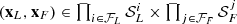 . In addition, let
  and
and  . Therefore, the profits
 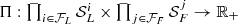 of each firm at the lower and upper levels may be written in terms of payoffs as:

 and
and  . It is worth noting that under Assumptions 2.2.1 and 2.2.2, the functions (2.2.1) and (2.2.2) are strictly concave.
The sequential game Γ displays two levels of decisions, namely 1 and 2, and no discounting. We also assume that the timing of positions is given.3 Each leader first chooses a quantity to sell, and each follower determines their supply based on the residual demand. Information is again assumed to be complete. Information is imperfect because at level 1 (resp. level 2) a leader (resp. a follower) cannot observe what the other leaders (resp. other followers) decide: the multiple leader–follower model is thus described by a two-stage game which embodies two simultaneous move partial games. Indeed, the leaders play a two-stage game with the followers, but the leaders (the followers) play a simultaneous move game together.
2.3 Stackelberg–Nash Equilibrium: A Definition
The main purpose of this section is to define the SNE. To this end, we study the optimal behavior in each stage of the bilevel game. In this framework, strategic interactions occur within each partial game but also between the partial games through sequential decisions. It is worth noting that the critical difference from the usual two-player games stem from the fact that the optimal decision made by a follower does not necessarily coincide with their best response.4
 and for all strategy profiles
  for all followers but j, we can define
  , with
  ,
, , as follower j’s optimal decision mapping. Thus, the lower level optimization problem for follower j may be written:5

 be the Lagrangian, where
  is the Kuhn–Tucker multiplier. By using Assumptions 2.2.1 and 2.2.2, the first-order sufficient condition may be written:
With Assumptions 2.2.1 and 2.2.2, the optimal decision mapping  exists and is unique.6 Indeed, we have either
  or
or  . Therefore, if
  , then λ = 0, where
  is the solution to the equation
  , which yields
  . Now, if λ > 0, then
  , which means that
  . Then,
  ,
,  . In addition, as for Assumptions 2.2.1 and 2.2.2,
  is strictly concave in
  , then, according to Berge Maximum Theorem,
  is continuously differentiable.

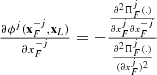 . We have that
  , when ϕ
j(.) > 0, and
, when ϕ
j(.) > 0, and  when ϕ
j(.) = 0. Then,
when ϕ
j(.) = 0. Then, ![$$\frac { \partial \phi ^{j}(.)}{\partial x_{F}^{-j}}\in (-1,0]$$](../images/480569_1_En_2_Chapter/480569_1_En_2_Chapter_TeX_IEq100.png) ,
,  . In addition, it is possible to show that
 ![$$\frac {\partial \phi ^{j}(.) }{\partial x_{L}^{i}}\in (-1,0]$$](../images/480569_1_En_2_Chapter/480569_1_En_2_Chapter_TeX_IEq102.png) ,
, 
 .
.We assume that the followers’ optimal behaviors as studied in stage 1 of the bilevel optimization process are consistent (see Sect. 2.4).7 Then, the system of equations which determines such best responses has a unique solution, so we can define the best response for follower j as  , with
  ,
,  .8 Let
  , with
  , be the vector of best responses. The vector function φ(x
L) constitutes a constraint for the decision maker at the upper level as we now have
, be the vector of best responses. The vector function φ(x
L) constitutes a constraint for the decision maker at the upper level as we now have  , where
  .
.
 , with
  , is the solution to the problem:
 be the Lagrangian, where
  is the Kuhn–Tucker multiplier. As
  , which is continuous (see Julien [22]), the Kuhn–Tucker conditions may be written:
The term  , with
  , represents the reaction of all followers to leader i’s strategy, i.e., the slope of the aggregate best response to i,
  . By construction, ν
i = ν
−i = ν for all
. By construction, ν
i = ν
−i = ν for all  . Let
. Let  . We may have either
  or
or  .
.
 , the second-order sufficient condition holds:
 , for each
  ; and, by using the implicit function theorem, we have that
![$$\frac {\partial \psi ^{j}(.)}{\partial x_{F}^{-j}} \in (-1,0]$$](../images/480569_1_En_2_Chapter/480569_1_En_2_Chapter_TeX_IEq127.png) , for all − i ≠ i,
, for all − i ≠ i,  .
.The solution to the n
L equations such as (2.3.5) yields the strategy profile for the leaders  . From the set of the best responses, i.e.,
  , it is possible to deduce the strategy profile for followers
  .
.
We are now able to provide a definition of an SNE for this bilevel game.
 , with
  , where φ :
  , such that conditions C1 and C2 hold:
 - C1

 ,
,  ,
,  and
and  ;
; - C2

 ,
,  . △
. △
2.4 Stackelberg–Nash Equilibrium: Existence and Uniqueness
Existence and uniqueness problems are complex in this framework as there are several decision makers at each level: strategic interactions occur within levels but also between the two levels through sequential decisions. Indeed, the n L leaders play a two-stage game with the n F followers, but the leaders (the followers) play a simultaneous move game together. Therefore, the bilevel game Γ displays two partial games, namely the lower level game Γ F and the upper level game Γ L. The equilibrium of the entire game Γ is a pure strategy subgame perfect Nash equilibrium (SPNE), while the equilibria in each partial game are Nash equilibria. We state two results which pertain to existence and uniqueness. Then, we discuss existence and uniqueness within the literature.
The following Theorem may be stated for the bilevel game Γ under consideration.
Let us consider the game Γ, and let Assumptions 2.2.1and 2.2.2be satisfied. Then, there exists a Stackelberg–Nash equilibrium.
△
Here we provide heuristic proof (for more details, see notably Julien [22] with weaker assumptions on costs). As we have many decision makers at the lower and upper levels, we show that there exists a Nash equilibrium at each level of the game, i.e., there exists a strategy profile  such that the leaders and followers strategic optimal plans are mutually consistent. We define the function
  , with
  . The function Λ(x
L) is continuous (as each ψ
i given by the solution for (2.3.5) is continuous under Assumptions 2.2.1 and 2.2.2 in x
L on
. The function Λ(x
L) is continuous (as each ψ
i given by the solution for (2.3.5) is continuous under Assumptions 2.2.1 and 2.2.2 in x
L on  , a compact and convex subset of Euclidean space (as the product of compact and convex strategy sets
  ,
,  ). Then, according to the Brouwer Fixed Point Theorem, the function Λ(x
L) has a fixed point
). Then, according to the Brouwer Fixed Point Theorem, the function Λ(x
L) has a fixed point  , with components
  , where
  , for each i
 . This fixed point is a pure strategy Nash equilibrium of the subgame Γ
L. Now let us define
. This fixed point is a pure strategy Nash equilibrium of the subgame Γ
L. Now let us define  , with
  , where, for each j, ϕ
j is the solution to (2.3.2). Given that
, where, for each j, ϕ
j is the solution to (2.3.2). Given that  , we have that
  . A similar argument as the one made for the leaders shows that the function
  has a fixed point
  , with components
  , where
  , for all
  . This fixed point is a pure strategy Nash equilibrium of the subgame Γ
F. But then, the point
. This fixed point is a pure strategy Nash equilibrium of the subgame Γ
F. But then, the point  , with
 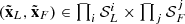 exists, which constitutes a SPNE of Γ. □
The existence of an equilibrium is obtained here under mild conditions for market demand and costs. Some of these conditions could be relaxed provided the remaining conditions are completed with additional restrictions. For instance, convexity of costs for all firms is not necessary.
The next theorem relies on the uniqueness of the SNE (see Julien [22]).
Let Assumptions 1 and 2 be satisfied. Then, if a Stackelberg–Nash equilibrium exists, it is unique. △
 (see Julien [22] for more details). Let
  , with
  , where
  . By using Corollary 2.1 in Kolstad and Mathiesen [26]), as leaders in the partial game Γ
L behave like Cournot firms, we show this criterion is satisfied, so the SNPE in Γ
L is unique. It is possible to show that:
. By using Corollary 2.1 in Kolstad and Mathiesen [26]), as leaders in the partial game Γ
L behave like Cournot firms, we show this criterion is satisfied, so the SNPE in Γ
L is unique. It is possible to show that: 
 , by using the assumptions on costs and demand, we deduce:
 there exists a unique Nash equilibrium in the subgame Γ
L. Now, given a unique point
there exists a unique Nash equilibrium in the subgame Γ
L. Now, given a unique point  , and by using a similar argument as the one made previously for the upper level, it is possible to show that
  at the lower level, with k = 1, in (2.4.1). Then, there is a unique pure strategy Nash equilibrium in the subgame Γ
F. Then, the SPNE of Γ is unique, which proves the uniqueness of the SNE. □
at the lower level, with k = 1, in (2.4.1). Then, there is a unique pure strategy Nash equilibrium in the subgame Γ
F. Then, the SPNE of Γ is unique, which proves the uniqueness of the SNE. □If we assume symmetry, the condition for the sign for  may be rewritten as
  , which would indicate that “on average” leaders’ marginal revenues could be increased but not too much. In addition,
  : the effect of a change in
  on i’s marginal profit dominates the sum of the cross effects of similar changes for the supply of other leaders. △
The uniqueness of an SNE holds under strong assumptions. It can happen that multiple Nash equilibria exist at both levels. At the lower level as well as the upper level, multiplicity of equilibria can be generated by strong strategic complementarities caused either by nonconvex costs or market demand functions which do not intersect the axis. The multiplicity of Nash equilibria can lead to coordination failures problems.
Existence and uniqueness have already been explored in the multiple leader–follower model. Sherali [33] shows existence and uniqueness with identical convex costs for leaders, and states some results under the assumptions of linear demand with either linear or quadratic costs (Ehrenmann [15]). Sherali’s model is an extension of the seminal paper by Murphy et al. [34] which covers the case of many followers who interact with one leader. In their model the authors provide a characterization of the SNE, along with an algorithm to compute it. They state a Theorem 1 which gives the properties of the aggregate best response for the followers expressed as a function of the leader’s strategy. This determination stems from a family of optimization programs for the followers based on a price function which is affected by the supply of the leader. They show that this aggregate function is convex, and then, study the problem faced by the leader. Nevertheless, they do not study the conditions under which the followers’ optimal decisions are mutually consistent. In the same vein, Tobin [37] provides an efficient algorithm to find a unique SNE by parameterizing the price function by the leader’s strategy. Some strong assumptions are made on the thrice-differentiability of the price function and the cost to the leader.
More recently, in line with De Wolf and Smeers [10] and DeMiguel and Xu [11] extend the work by Sherali [33] to include uncertainty with stochastic market demand. Unlike Sherali [33] they allow costs to differ across leaders. Nevertheless, to show that the expected profit of any leader is concave, they assume that the aggregate best response of the followers is convex. However as this assumption does not always hold, these authors must resort to a linear demand. Pang and Fukushima [31], Yu and Wang [40], and Jia et al. [20] prove the existence of an equilibrium point of a finite game with two leaders and several followers without specifying the assumptions made on demand and costs. Kurkarni and Shanbhag [27] show that when the leaders’ objectives admit a quasi-potential function, the global and local minimizers of the leaders’ optimization problems are global and local equilibria of the game. Finally, Aussel et al. [2] study the existence of an equilibrium in the electricity markets.
2.5 The Linear and the Quadratic Bilevel Optimization Games
In this section, we consider two standard bilevel optimization games: the linear model with asymmetric costs and the quadratic model with symmetric costs. The following specification holds in both models. There are  leader(s) and
  follower(s), with n
L + n
F = n. Let p(X) = a − bX, a, b > 0, where X ≡ X
L + X
F, with
follower(s), with n
L + n
F = n. Let p(X) = a − bX, a, b > 0, where X ≡ X
L + X
F, with  and
and  .
.
2.5.1 The Linear Bilevel Optimization Game
The costs functions are given by  , i = 1, …, n
L, and by
, i = 1, …, n
L, and by  , j = 1, …, n
F, with
, j = 1, …, n
F, with  , for all i and all j. The strategy sets are given by
 ![$$\mathcal {S}_{L}^{i}=[0,\frac {a}{b} -c_{L}^{i}],i\in \mathcal {F}_{L}$$](../images/480569_1_En_2_Chapter/480569_1_En_2_Chapter_TeX_IEq183.png) , and
, and![$$\mathcal {S}_{F}^{j}=[0,\frac {a}{b} -c_{F}^{j}]$$](../images/480569_1_En_2_Chapter/480569_1_En_2_Chapter_TeX_IEq184.png) ,
,  .
.
 and
and  , where
  . The corresponding payoffs are given by
  (resp.
  ) when
  (resp.
  ). In addition, the Cournot–Nash equilibrium (CNE), in which all firms play simultaneously, is given by
  ,
,  ,
,  ,
,  ,
,  , and
, and  , with corresponding payoffs
![$$\displaystyle \begin{aligned} \phi ^{j}({\mathbf{x}}_{F}^{-j},{\mathbf{x}}_{L}\mathbf{)}:\max \{[a-b(x_{F}^{j}+X_{F}^{-j}+X_{L})-c_{F}^{j}x_{F}^{j}]x_{F}^{j}:\mathcal{S} _{F}^{j}=[0,\frac{a}{b}-c_{F}^{j}]\}\text{.}\ {} \end{aligned} $$](../images/480569_1_En_2_Chapter/480569_1_En_2_Chapter_TeX_Equ12.png)

 . The best response for follower j,
  , is given by the convex linear function:
 , leader i’s optimal decision mapping
  is the solution to the upper level optimization problem, which may be written as follows:
 ![$$\displaystyle \begin{aligned} \psi ^{i}({\mathbf{x}}_{L}^{-i}\mathbf{)}:\max \left\{\left[ \frac{ a+\sum_{j}c_{F}^{j}}{n_{F}+1}-\frac{b(x_{L}^{i}+X_{L}^{-i})}{n_{F}+1} -c_{L}^{i}\right] x_{L}^{i}:\mathcal{S}_{L}^{i}=[0,\frac{a}{b}-c_{L}^{i}]\right\} \text{.} {} \end{aligned} $$](../images/480569_1_En_2_Chapter/480569_1_En_2_Chapter_TeX_Equ15.png)


 , so the market price is given by:
![$$\displaystyle \begin{aligned} \tilde{\Pi}_{L}^{i}=\frac{A[a-(n_{F}+1)c_{L}^{i}+\sum_{j}c_{F}^{j}]}{ b(n_{L}+1)^{2}(n_{F}+1)}\text{, }i\in \mathcal{F}_{L}\text{;} {} \end{aligned} $$](../images/480569_1_En_2_Chapter/480569_1_En_2_Chapter_TeX_Equ20.png)
![$$\displaystyle \begin{aligned} \tilde{\Pi}_{F}^{j}=\frac{B[a-(n_{F}+1)c_{F}^{j}-n_{L} \sum_{j}c_{F}^{j}+(n_{F}+1)\sum_{i}c_{L}^{i}]}{b[(n_{L}+1)(n_{F}+1)]^{2}} \text{, }j\in \mathcal{F}_{F}\text{,} {} \end{aligned} $$](../images/480569_1_En_2_Chapter/480569_1_En_2_Chapter_TeX_Equ21.png)
 and
and  .
.Finally, consider the particular case where  , i = 1, …, n
L, and by
, i = 1, …, n
L, and by  , j = 1, …, n
F , with c < a. The CE, is such that aggregate supply and market price are given respectively by
, j = 1, …, n
F , with c < a. The CE, is such that aggregate supply and market price are given respectively by  , p
∗ = c, and ( Πi)∗ = 0, i = 1, …, n.9 The CNE is given by
, p
∗ = c, and ( Πi)∗ = 0, i = 1, …, n.9 The CNE is given by  ,
,  ,
,  , and
, and  ,
,  ,
,  . The SNE is given by
  ,
,  ,
,  ,
,  ,
, ![$$\tilde {p}=\frac { a+c\left [ n_{L}(n_{F}+1)+n_{F}\right ] }{(n_{L}+1)(n_{F}+1)}$$](../images/480569_1_En_2_Chapter/480569_1_En_2_Chapter_TeX_IEq222.png) ,
,  ,
,  , and
, and ![$$\tilde {\Pi }_{F}^{j}=\frac {(a-c)^{2}}{b[(n_{L}+1)(n_{F}+1)]^{2}}$$](../images/480569_1_En_2_Chapter/480569_1_En_2_Chapter_TeX_IEq225.png) ,
,  .
.
We can observe that for each  , we have
  whenever
  : any leader will achieve a higher payoff provided the number of leaders is not too high.10 It is worth noting that
  (resp.
  ): so when the number of leaders (resp. leaders and followers) becomes arbitrarily large the SNE market price coincides with the CE price p
∗. This result holds with the CNE in case either the number of leaders or followers goes to infinity (in the inclusive sense!).
): so when the number of leaders (resp. leaders and followers) becomes arbitrarily large the SNE market price coincides with the CE price p
∗. This result holds with the CNE in case either the number of leaders or followers goes to infinity (in the inclusive sense!).
2.5.2 The Quadratic Bilevel Optimization Game
The costs functions are given by  , i = 1, …, n
L, and by
, i = 1, …, n
L, and by  , j = 1, …, n
F, with c < a, for all i and all j. The strategy sets are given by
, j = 1, …, n
F, with c < a, for all i and all j. The strategy sets are given by ![$$\mathcal {S}_{L}^{i}=[0,\frac {a}{b}-\frac {c}{2} (x_{L}^{i})^{2}],i\in \mathcal {F}_{L}$$](../images/480569_1_En_2_Chapter/480569_1_En_2_Chapter_TeX_IEq234.png) , and
, and![$$\mathcal {S}_{F}^{j}=[0,\frac {a}{b }-\frac {c}{2}(x_{L}^{i})^{2}]$$](../images/480569_1_En_2_Chapter/480569_1_En_2_Chapter_TeX_IEq235.png) ,
,  .
.
The CNE is given by  , for all
  ,
,  , for all
  ,
,  , and
, and ![$$\hat {\Pi }_{L}^{i}=\frac {a^{2}(2b+c)}{[b(n_{L}+n_{F}+1)+c]^{2}}$$](../images/480569_1_En_2_Chapter/480569_1_En_2_Chapter_TeX_IEq242.png) , for all
, for all  ,
, ![$$\hat {\Pi }_{F}^{j}=\frac {a^{2}(2b+c)}{ [b(n_{L}+n_{F}+1)+c]^{2}}$$](../images/480569_1_En_2_Chapter/480569_1_En_2_Chapter_TeX_IEq244.png) , for all
, for all  .
.

![$$\displaystyle \begin{aligned} \tilde{x}_{F}^{j}=\frac{a[b+c(1+\frac{b}{b+c}n_{F})]}{ [c+b(n_{F}+1)][b(n_{L}+1)+c(\frac{b}{b+c}n_{F}+1)]}\text{, }j\in \mathcal{F} _{F}. {} \end{aligned} $$](../images/480569_1_En_2_Chapter/480569_1_En_2_Chapter_TeX_Equ23.png)
![$$\displaystyle \begin{aligned} \tilde{p}=\frac{a(b+c)[b+c(1+\frac{b}{b+c}n_{F})]}{ [c+b(n_{F}+1)][b(n_{L}+1)+c(\frac{b}{b+c}n_{F}+1)]}. {} \end{aligned} $$](../images/480569_1_En_2_Chapter/480569_1_En_2_Chapter_TeX_Equ24.png)
![$$\displaystyle \begin{aligned} \tilde{\Pi}_{L}^{i}=\frac{a^{2}(2b^{2}+3bc+c^{2}+bcn_{F})}{ 2[c+b(n_{F}+1)][b(n_{L}+1)+c(\frac{b}{b+c}n_{F}+1)]^{2}}\text{, }i\in \mathcal{F}_{L}, {} \end{aligned} $$](../images/480569_1_En_2_Chapter/480569_1_En_2_Chapter_TeX_Equ25.png)
![$$\displaystyle \begin{aligned} \tilde{\Pi}_{F}^{j}=\frac{a^{2}(2b+c)[b+c(1+\frac{b}{b+c}n_{F})]^{2}}{ 2[c+b(n_{F}+1)]^{2}[b(n_{L}+1)+c(\frac{b}{b+c}n_{F}+1)]^{2}}\text{, }j\in \mathcal{F}_{F}. {} \end{aligned} $$](../images/480569_1_En_2_Chapter/480569_1_En_2_Chapter_TeX_Equ26.png)
It is easy to check that, as the production of any leader is higher than the production of any follower, the payoff of any leader is higher.
2.6 Stackelberg–Nash Equilibrium: Welfare Properties
We now turn to the nonoptimality of the SNE and some of its welfare properties. To this end, we compare the SNE market outcome with the CNE, and with the CE. Next, we consider the relation between market concentration and surplus, and also the relation between individual market power, payoffs and mergers.
2.6.1 The SNE, CNE and CE Aggregate Market Outcomes
We can state the following proposition, which represents a well-known result.
Let
 ,
,  , and X
∗be respectively the SNE, the CNE, and the CE aggregate supplies; and
, and X
∗be respectively the SNE, the CNE, and the CE aggregate supplies; and
 ,
,  , and p
∗the corresponding market prices. Then,
, and p
∗the corresponding market prices. Then,
 , and
, and
 . △
. △
In the bilevel optimization game, the leaders can set a higher supply. In addition, the increment in the aggregate supply of leaders more than compensates for the decrease in the aggregate supply of followers when the aggregate best response is negatively sloped, whereas it goes in the same direction when the aggregate best response increases, i.e., when strategies are complements.11 Therefore, the aggregate supply (market price) is higher (lower) in the SNE than in the CNE, both when strategies are substitutes and when they are complements. The following example illustrates that the noncooperative sequential game leads to higher traded output than in the noncooperative simultaneous game (see Daughety [9]).
Consider the linear bilevel game given by (2.5.1)–(2.5.10), where  , i = 1, …, n
L, and by
, i = 1, …, n
L, and by  , j = 1, …, n
F, with c < a. From (2.5.6) and (2.5.7), we can deduce
, j = 1, …, n
F, with c < a. From (2.5.6) and (2.5.7), we can deduce  and
and  . Then, the aggregate supply is
  , which may be written as
  . We see that
  . Then, we obtain
 ![$$p^{\ast }<\tilde {p}=\frac {a+c\left [ n_{L}(n_{F}+1)+n_{F}\right ] }{(n_{L}+1)(n_{F}+1)}$$](../images/480569_1_En_2_Chapter/480569_1_En_2_Chapter_TeX_IEq259.png) . We can observe that
. We can observe that  , which corresponds to the Cournot–Nash equilibria, and
  . Then, for fixed n, the aggregate supply is concave in n
L, i.e.,
. Then, for fixed n, the aggregate supply is concave in n
L, i.e.,  . Indeed, the Cournot–Nash aggregate supply is given by
  . Then, we have
  .
.
When the aggregate best response for followers has a zero slope in equilibrium, the leaders rationally expect that each strategic decision they undertake should entail no reactions from the followers (Julien [21]). △
2.6.2 Welfare and Market Power
 , with
  , and
, and  , with
  , and where 𝜗
L + 𝜗
F = 1. Therefore, the social surplus may be defined as:
, and where 𝜗
L + 𝜗
F = 1. Therefore, the social surplus may be defined as: 
 is leader i’s market share, and
  is follower j’s market share. Differentiating partially with respect to X and decomposing p(X) leads to:
 , and for fixed
  ,
,  , 𝜗
L and 𝜗
F, with
, 𝜗
L and 𝜗
F, with  .
.The social surplus is hence higher at the SNE than at the CNE, and reaches its maximum value at the CE.12 Therefore, one essential feature of the SNE bilevel game is that the strategic interactions between leaders and followers may be welfare enhancing.
Daughety [9] shows that, if the aggregate supply is used as a measure of welfare, welfare may be maximized when there is considerable asymmetry in the market, whereas symmetric (Cournot) equilibria for which n L = 0 and n L = n minimize welfare. Thus, the concentration index may no longer be appropriate for measuring welfare. △
2.6.3 Market Power and Payoffs


 and
and  are leader i’s and follower j’s markups, and 𝜖 is the price elasticity of demand, that is,
  .
.

 and
and  are the Lerner indexes for follower j and for leader i respectively.13
If
 , then
 ,
,  ,
,  . In addition, if
 for all
 and
and
 , then,
 if and only if
 ,
,  ,
,  . △
. △
It is worth pointing out that there are certain differences in leaders’ (resp. followers’) payoffs caused by asymmetries in costs. As this bilevel game embodies strategic interactions among several leaders and followers, we now explore the possibility of merging.
2.6.4 Welfare and Mergers
The strategic effects of merging on welfare depend on the noncooperative strategic behavior which prevails in the SNE. The following example illustrates the welfare effects of merging (see Daughety [9]).
 , i = 1, …, n
L, and by
, i = 1, …, n
L, and by  , j = 1, …, n
F, with c < a. Let
, j = 1, …, n
F, with c < a. Let  . First, a merger means that one firm disappears from the market. Consider the following three cases:
 - 1.
The merger of two leaders so that the post merger market has n L − 1 leaders but still n − n L followers;
- 2.
The merger of two followers, so that there are n L leaders but n − n L − 1 followers; and
- 3.
The merger of one leader and one follower, so that there are n L leaders but n − n L − 1 followers.

 . Thus, welfare is always reduced. Second, if we now consider that the number of leaders increases, the comparative statics yields:


 whenever
  : so, when there are few leaders, merging can increase aggregate supply. More asymmetry is beneficial; it is socially desirable as it enhances welfare. However when
  , fewer leaders and more followers could increase welfare.
The difference between the two cases can be explained by the fact that, in the second case, the reduction of the number of followers is associated with an increase in the number of leaders.
It can be shown that two firms which belong to the same cohort and have the same market power rarely have an incentive to merge, whereas a merger between two firms which belong to two distinct cohorts and have different levels of market power is always profitable as the leader firm incorporates the follower firm regardless of the number of rivals. In the SNE the merger better internalizes the effect of the increase in price on payoffs than in the CNE: the decrease in supply is lower than under Cournot quantity competition. △
2.7 Extension to Multilevel Optimization
Bilevel optimization models have been extended to three-level optimization environments (see Bard and Falk [6], Benson [7], Han et al. [17, 18], among others), and to T-level optimization with one decision maker at each level (Boyer and Moreaux [8], Robson [32]). The three level optimization game has been studied in depth by Alguacil et al. [1] and Han et al. [17]. The existence of a noncooperative equilibrium in the multilevel optimization with several decision makers at each level remains an open problem. Nevertheless, the multiple leader–follower game may be extended to cover a T-stage decision setting in the case of the linear model (Watt [39], Lafay [28], and Julien et al. [24, 25]). The extended game should represent a free entry finite horizon hierarchical game. We will focus on the computation and on certain welfare properties. To this end, and for the sake of simplicity, we consider an extended version of the linear model studied in Sect. 2.5, where  , i = 1, …, n
L, and by
, i = 1, …, n
L, and by  , j = 1, …, n
F, with c < a.
, j = 1, …, n
F, with c < a.
There are now T levels of decisions indexed by t, t = 1, 2, …, T. Each level embodies n
t decision makers, with  . The full set of sequential levels represents a hierarchy. The supply of firm i in level t is denoted by
  . The aggregate supply in level t is given by
  . The n
t firms behave as leaders with respect to all firms at levels τ > t, and as followers with respect to all firms at levels τ < t. The price function may be written as p = p(∑tX
t). Let p(X) = a − bX, a, b > 0, where X ≡∑tX
t. The costs functions are given by
. The n
t firms behave as leaders with respect to all firms at levels τ > t, and as followers with respect to all firms at levels τ < t. The price function may be written as p = p(∑tX
t). Let p(X) = a − bX, a, b > 0, where X ≡∑tX
t. The costs functions are given by  , i = 1, …, n
t, t = 1, …, T, with c < a. The strategy sets are given by
, i = 1, …, n
t, t = 1, …, T, with c < a. The strategy sets are given by ![$$\mathcal {S}_{t}^{i}=[0,\frac {a}{b}-c]$$](../images/480569_1_En_2_Chapter/480569_1_En_2_Chapter_TeX_IEq309.png) , i = 1, …, n
t, t = 1, …, T.
, i = 1, …, n
t, t = 1, …, T.
Bearing in mind this framework, if firms compete as price-takers, the CE is still given by  , p
∗ = c, and
, p
∗ = c, and  , i = 1, …, n
t, t = 1, …, T. The CNE is given by
, i = 1, …, n
t, t = 1, …, T. The CNE is given by  ,
,  ,
,  , and
, and  , i = 1, …, n
t, t = 1, …, T.
, i = 1, …, n
t, t = 1, …, T.
![$$\displaystyle \begin{aligned} \Pi _{t}^{i}(x_{t}^{i},X_{t}^{-i},\sum_{\tau ,\tau \neq t}^{T}X_{\tau })=[a-b(x_{t}^{i}+X_{t}^{-i}+\sum_{\tau ,\tau \neq t}^{T}X_{\tau })]x_{F}^{j}-cx_{F}^{j}\text{.}\ {} \end{aligned} $$](../images/480569_1_En_2_Chapter/480569_1_En_2_Chapter_TeX_Equ33.png)
![$$\displaystyle \begin{aligned} \underset{\{x_{t}^{i}\}}{\max }\Pi _{t}^{i}(x_{t}^{i},X_{t}^{-i},\sum_{\tau =1}^{t-1}X_{t-\tau },\sum_{\tau =1}^{T-t}X_{t+\tau }):=[a-c-b(x_{t}^{i}+X_{t}^{-i}+\sum_{\tau =1}^{t-1}X_{t-\tau }+\sum_{\tau =1}^{T-t}X_{t+\tau })]x_{t}^{i}\text{,} {} \end{aligned} $$](../images/480569_1_En_2_Chapter/480569_1_En_2_Chapter_TeX_Equ34.png)
 , and
, and  and
and  denote respectively the aggregate supply of all leaders at level t − τ for τ ∈{1, …, t − 1} and the aggregate supply of all followers at level t + τ for τ ∈{1, …, T − t}.
 . By solving recursively from the last level T to the first level 1, it is possible to deduce the equilibrium strategy for any firm at any stage (see Watt [39]). Indeed, the SNE strategy of firm i at stage t may be written as follows:14


It is worth noting that the specification T = 2, n t = 1, t = 1, 2, corresponds to the standard bilevel duopoly game. The specification T = 2, n 1 = n L and n 2 = n F, corresponds to the linear bilevel game from Sect. 2.5.
Consider a market with linear demand and identical constant marginal costs, then the T-level Stackelberg game coincides with a multilevel Cournot game in which firms compete oligopolistically on the residual demands.
△
See Julien et al. [25] who show that the assumptions of linear demand and identical (strictly positive) constant marginal costs are necessary and sufficient conditions for Proposition 2.7.1 to hold. □
Therefore each firm within a given stage behaves as if there were no subsequent stages, i.e., it is as if the direct followers for firm i in stage t do not matter. This generalizes the t-stage monopoly property of Boyer and Moreaux [8].
 , as:
, as: 
Then, we are able to state the following two propositions (see Julien et al. [24]).
When the number of firms becomes arbitrarily large, either by arbitrarily increasing the number of firms at each stage by keeping the number of stages T constant, i.e., ∀t, n t →∞, given T < ∞ , or by increasing the number of stages without limit, i.e., T →∞, the T-level SNE aggregate supply converges to the CE aggregate supply. △
Immediate from the two limits given by limT→∞(  and
and  (
( . □
. □
In the T-level linear economy, social welfare can be maximized by enlarging the hierarchy or by changing the size of existing stages through the reallocation of firms from the most populated stage until the size of all stages is equalized. △
See Julien et al. [24]. The relocation reflects the merger analysis provided in Daughety [9] (see preceding subsection). When the number of levels is fixed, the relocation is welfare improving until there is the same number of firms at each level. □
A sequential market structure with one firm per stage Pareto dominates any other market structure, including the CNE (see Watt [39]). △
It can be verified that the firms’ surplus in the SNE may be inferior to the firms’ surplus in the CNE when  , so the firm which chooses to be at the upper level may be better off if the other firms are supplying simultaneously. △

 , with
  , represents the supply of the additional firm. In addition, the maximization of welfare implies the most asymmetric distribution of market power. Nevertheless, these results are valid in a linear economy with identical costs. Indeed, if costs are different, entry is affected by some relocations or extensions. Lafay [28] uses a T-level game in which firms enter at different times or have different commitment abilities. Here firms bear different constant marginal costs. The linearT- level optimizationgame confirms the positive effect of an increase in the number of decision makers on welfare. However, the salient feature is that firms must now forecast future entries in the market. Indeed, asymmetric costs could make entry inefficient. If the firm reasons backwards, and the price is lower when there is further entry, the firm enters the market provided its costs do not exceed the resulting market price.15
2.8 Conclusion
We have proposed a short synthesis of the application of bilevel optimization to some simple economic problems related to oligopolistic competition. Using standard assumptions in economics relative to the differentiability of objective functions, we have presented some elements to characterize the Stackelberg–Nash equilibrium of the noncooperative two-stage game, where the game itself consists of two Cournot simultaneous move games embedded in a Stackelberg sequential competition game.
The tractability of the model, especially when assuming linearity of costs and demand, makes it possible to derive certain welfare implications from this bi-level optimization structure, and to compare it with standard alternatives in terms of market structures. Indeed, the T-level optimization game represents a challenge to the modeling of strategic interactions.
The authors acknowledge an anonymous referee for her/his helpful comments, remarks and suggestions on an earlier version. Any remaining deficiencies are ours.