S. Dempe, A. Zemkoho (eds.)Bilevel OptimizationSpringer Optimization and Its Applications161https://doi.org/10.1007/978-3-030-52119-6_4

4. Regularization and Approximation Methods in Stackelberg Games and Bilevel Optimization

Francesco Caruso¹, M. Beatrice Lignola² and Jacqueline Morgan³

(1)

Department of Economics and Statistics, University of Naples Federico II, Naples, Italy

(2)

Department of Mathematics and Applications R. Caccioppoli, University of Naples Federico II, Naples, Italy

(3)

Department of Economics and Statistics & Center for Studies in Economics and Finance, University of Naples Federico II, Naples, Italy

Francesco Caruso

Email: francesco.caruso@unina.it

M. Beatrice Lignola

Email: lignola@unina.it

Jacqueline Morgan (Corresponding author)

Email: morgan@unina.it

Abstract

In a two-stage Stackelberg game, depending on the leader’s information about the choice of the follower among his optimal responses, one can associate different types of mathematical problems. We present formulations and solution concepts for such problems, together with their possible roles in bilevel optimization, and we illustrate the crucial issues concerning these solution concepts. Then, we discuss which of these issues can be positively or negatively answered and how managing the latter ones by means of two widely used approaches: regularizing the set of optimal responses of the follower, via different types of approximate solutions, or regularizing the follower’s payoff function, via the Tikhonov or the proximal regularizations. The first approach allows to define different kinds of regularized problems whose solutions exist and are stable under perturbations assuming sufficiently general conditions. Moreover, when the original problem has no solutions, we consider suitable regularizations of the second-stage problem, called inner regularizations, which enable to construct a surrogate solution, called viscosity solution, to the original problem. The second approach permits to overcome the non-uniqueness of the follower’s optimal response, by constructing sequences of Stackelberg games with a unique second-stage solution which approximate in some sense the original game, and to select among the solutions by using appropriate constructive methods.

Keywords

Stackelberg gameBilevel optimization problemSubgame perfect Nash equilibrium problemApproximate solutionInner regularization and viscosity solutionTikhonov regularizationProximal point method

4.1 Introduction

In this chapter we are interested in describing interactions that could occur between two agents (or players) which act sequentially in two stages. More precisely, we consider that

1.
in the first stage: one player, henceforth called the leader, chooses an action x in his action set X;
2.
in the second stage: one player, henceforth called the follower, observes the action x chosen by the leader in the first stage and then chooses an action y in his action set Y ;
3.
after the two-stage interaction: the leader receives L(x, y) where $L\colon X\times Y\to \mathbb {R}$ is the leader’s payoff function, and the follower receives F(x, y) where $F\colon X\times Y\to \mathbb {R}$ is the follower’s payoff function.

Such a situation defines a Stackelberg game, denoted by Γ = (X, Y, L, F), which has been modelled for the first time by von Stackelberg in [109] in an economic framework.

Assume that players aim to minimize their payoff functions, as traditionally used in optimization literature where the payoff functions embed players’ costs. However, since $\max f(\cdot )=-\min \{-f(\cdot )\}$ , we could assume equivalently that players maximize their payoff functions (which usually appears in economics contexts, where payoff functions represent players’ profits). At the moment, we set no assumptions on the structure of the actions sets X and Y : they could be of finite or infinite cardinalities, subsets of finite or infinite dimensional spaces, strict subsets or whole spaces, etc. Their nature will be specified each time in the sequel of the chapter.

The follower, once he has seen the action x chosen by the leader, faces the optimization problem

$\displaystyle \begin{aligned} (P_x)\colon\min_{y\in Y} F(x,y), \end{aligned}$

i.e. finding y ∈ Y such that F(x, y) =inf_{z ∈ Y}F(x, z). Then, he reacts to the leader’s choice by picking an optimal response to x, that is an action belonging to the set, called the follower’s optimal reaction set

$\displaystyle \begin{aligned} {M}(x)=\operatorname*{\mbox{Arg min}}_{y\in Y}F(x,y)=\left\{y\in Y \text{ such that } F(x,y)=\inf_{z\in Y}F(x,z)\right\}. \end{aligned}$

The set-valued map $M\colon X\rightrightarrows Y$ that assigns to any action x of the leader the set M(x) defined above is the follower’s best reply correspondence. For sake of brevity, it will be also called argmin map.

The leader, if he can foresee the optimal response $y(x)\in \operatorname *{\mbox{Arg min}}_{y\in Y}F(x,y)$ chosen for any action x by the follower, will pick an action in the set $\operatorname *{\mbox{Arg min}}_{x\in X}L(x,y(x))$ according to such a forecast.

Given the informative structure of the game, predicting the follower’s optimal responses (or, equivalently, the response function y(⋅) of the follower) is typically a hard task for the leader, unless some additional information is available. Therefore, depending on the additional information of the leader about the single-valuedness of M or, when M is not single-valued, about how the follower chooses an optimal response in the set M(x) for any x ∈ X, one can associate to the Stackelberg game Γ different kinds of mathematical problems.

In Sect. 4.2 such mathematical problems and the related solution concepts are presented, together with illustrative examples and their possible roles in bilevel optimization.

In Sect. 4.3 we describe and discuss the main crucial issues arising in the just mentioned problems, focusing on the following ones: existence of solutions, “variational” stability, well-posedness, approximation, numerical approximation and selection of solutions. The crucial issues negatively answered are illustrated by counterexamples.

In order to overcome the drawbacks connected to the (negatively answered) crucial issues, two basic and widely used approaches are identified. They lead to two classes of regularization methods which allow to obtain key-properties for the regularized problems which, in general, are not satisfied in the original problem.

Regularizing the follower’s optimal reaction sets;
Regularizing the follower’s payoff function.

In Sect. 4.4 the first of the above approaches is presented and investigated for some of the problems defined in Sect. 4.2, and also for other types of two-stage games where the second-stage problem to solve is defined by a variational or a quasi-variational inequality, by a Nash equilibrium problem or by a quasi-equilibrium problem. Such an approach permits to define different kinds of regularized problems whose solutions exist and are stable under perturbations assuming sufficiently general conditions. Moreover, when the original problem has no solutions, we present suitable regularizations of the second-stage problem, called inner regularizations, which allow to construct a surrogate solution, called viscosity solution, to the original problem.

In Sect. 4.5 we investigate the second approach, that enables both to overcome the non-uniqueness of the follower’s optimal response and to select among the solutions. To get these goals, we construct sequences of Stackelberg games with a unique second-stage solution which approximate in some sense the original game by exploiting first the Tikhonov regularization and then the proximal regularization, two well-known regularization techniques in convex optimization.

A conclusive section concerns various extensions of the Stackelberg game notion considered in this chapter.

4.2 Models and Solution Concepts

We will illustrate five problems and solution concepts connected to the Stackelberg game defined in the previous section. The first one appears if the follower’s best reply correspondence M is assumed to be single-valued (and the leader knows it), whereas the others concern situations where M is not single-valued. Their connections will be emphasized and illustrated by examples. In this section, we only refer to seminal papers and to the first ones on regularization and approximation methods.

4.2.1 Stackelberg Problems

When the follower’s optimal response to any choice of the leader is unique, the leader can fully anticipate the reaction of the follower taking this into account before choosing his action and the follower behaves answering to the leader in the optimal (expected) way. Therefore, assumed that M is single-valued and M(x) = {m(x)} for any x ∈ X, the leader faces the so-called Stackelberg problem

$\displaystyle \begin{aligned} (SP)\, \begin{cases} \underset{x\in X}{\min}\,\,L(x,m(x)) \\ \text{where } m(x) \text{ is the solution to }(P_x). \end{cases} \end{aligned}$

The players acting in this way are often referred to be engaged in a classical Stackelberg game, terminology due to von Stackelberg who first investigated such an interaction in [109] where an economic model involving two firms that compete sequentially on quantities to produce is presented. Then, properties of Stackelberg solutions together with extensions of the classical Stackelberg games to a dynamic framework have been investigated in [24, 105].

Let us recall the solution concepts associated to (SP).

Definition 4.2.1

The infimum value inf_{x ∈ X}L(x, m(x)) is the Stackelberg value of (SP).
A leader’s action $\bar x\in X$ is a Stackelberg solution to (SP) if
$\displaystyle \begin{aligned} \bar x\in \operatorname*{\mbox{Arg min}}_{x\in X}L(x,m(x)). \end{aligned}$
An action profile $(\bar x,\bar y)\in X\times Y$ is a Stackelberg equilibrium of (SP) if $\bar x$ is a Stackelberg solution and $\bar y=m(\bar x)$ . △

Stackelberg Leadership Model

The Stackelberg leadership model described in [109] regards two firms in a market which sell homogeneous products and have to choose the quantities to produce. Firm 1, acting as the leader, chooses first a quantity q ₁ ≥ 0; then firm 2, acting as the follower, observes the quantity q ₁ and chooses a quantity q ₂ ≥ 0. The firms aim to maximize their profit functions defined on [0, +∞[² by

$\displaystyle \begin{aligned} L(q_1,q_2)=q_1P(Q)-C_1(q_1)\quad \text{and}\quad F(q_1,q_2)=q_2P(Q)-C_2(q_2), \end{aligned}$

respectively, where Q = q ₁ + q ₂ is the total quantity in the market, P(⋅) is the inverse demand function and C _i(⋅) is the cost function of firm i ∈{1, 2}. As often happens in economics contexts, we assume linear inverse demand function $P(Q)=\max \{0,a-bQ\}$ with a, b ∈ ]0, +∞[ and linear cost functions C _i(q _i) = cq _i for any i ∈{1, 2} with c ∈ ]0, a[. Hence, the optimal response of firm 2 to any quantity chosen by firm 1 is unique and given by

$\displaystyle \begin{aligned} m(q_1)=\max\left\{0,\frac{a-bq_1-c}{2b}\right\},\quad \text{for any }q_1\in[0,+\infty[ \end{aligned}$

and, since $\operatorname *{\mbox{Arg max}}_{q_1\in [0,+\infty [}L(q_1,m(q_1))=\{(a-c)/2b\}$ , the quantities produced at equilibrium are

$\displaystyle \begin{aligned} \bar q_1=\frac{a-c}{2b}\quad \text{and}\quad \bar q_2=\frac{a-c}{4b}. \end{aligned}$

In Stackelberg leadership models the equilibrium quantity of the firm acting as the leader is always greater than equilibrium quantity of the firm acting as the follower (analogously for the equilibrium profits).

We point out that in [67, 72, 103] the following more general Stackelberg problem has been treated:

$\displaystyle \begin{aligned} (GSP)\, \begin{cases} \underset{x\in X,\,g(x,m(x))\leq 0}{\min}\,\,L(x,m(x)) \\ \mbox{where } m(x) \mbox{ is the solution to }(P_x), \end{cases} \end{aligned}$

where $g\colon X\times Y\to \mathbb {R}$ . In such a problem the leader’s constraints depend also on the follower’s best reply function m, which makes it harder to manage than (SP) from the mathematical point of view. In the sequel of the chapter we will consider only constraints for the leader which do not depend on the actions of the follower.

From now on, in the next subsections of this section we assume that M is not single-valued.

4.2.2 Pessimistic Leader: Weak Stackelberg Problem

Firstly, we consider an “extreme” situation where the pessimistic leader believes that the follower could choose the worst action for him in the set of optimal responses. The leader, who would prevent himself against the worst he can obtain when the follower plays optimally, will face the weak Stackelberg problem, also called pessimistic bilevel optimization problem

$\displaystyle \begin{aligned} (PB) \,\begin{cases} \underset{x\in X}{\min}\,\,\underset{y\in {M}(x)}{\sup}\,\,L(x,y) \\ \mbox{where }{M}(x)=\underset{y\in Y}{\operatorname*{\mbox{Arg min}}}\,\,F(x,y). \end{cases} \end{aligned}$

One of the first investigations of such a problem is due to Leitmann in [46], where it is denoted as generalized Stackelberg problem. The solution concepts associated to (PB) are reminded below.

Definition 4.2.2

The infimum value w =inf_{x ∈ X}sup_{y ∈ M(x)}L(x, y) is the security (or pessimistic) value of (PB).
A leader’s action $\bar x\in X$ is a weak Stackelberg (or pessimistic) solution to (PB) if
$\displaystyle \begin{aligned} \bar x\in\operatorname*{\mbox{Arg min}}_{x\in X}\sup_{y\in M(x)} L(x,y), \end{aligned}$
that is, $\sup _{y\in M(\bar x)} L(\bar x,y)=\inf _{x\in X}\sup _{y\in M(x)} L(x,y)$ .
An action profile $(\bar x,\bar y)\in X\times Y$ is a weak Stackelberg (or pessimistic) equilibrium of (PB) if $\bar x$ is a weak Stackelberg solution and $\bar y\in M(\bar x)$ . △

For first investigations about regularization and approximation of problem (PB) see [51, 69, 71, 89].

4.2.3 Optimistic Leader: Strong Stackelberg Problem

In a second “extreme” situation, the leader is optimistic and believes that the follower will choose the best action for the leader in the set of his optimal responses (or the leader is able to force the follower to choose, among all the optimal responses, the best one for the leader). The leader will deal with the strong Stackelberg problem, also called optimistic bilevel optimization problem

$\displaystyle \begin{aligned} (OB) \,\begin{cases} \underset{x\in X}{\min}\,\,\underset{y\in {M}(x)}{\inf}\,\,L(x,y) \\ \text{where }{M}(x)=\underset{y\in Y}{\operatorname*{\mbox{Arg min}}}\,\,F(x,y). \end{cases} \end{aligned}$

The solution concepts associated to (OB) are reminded below.

Definition 4.2.3

The infimum value s =inf_{x ∈ X}inf_{y ∈ M(x)}L(x, y) is the optimistic value of (OB).
A leader’s action $\bar x\in X$ is a strong Stackelberg (or optimistic) solution to (OB) if
$\displaystyle \begin{aligned} \bar x\in\operatorname*{\mbox{Arg min}}_{x\in X}\inf_{y\in M(x)} L(x,y), \end{aligned}$
that is, $\inf _{y\in M(\bar x)} L(\bar x,y)=\inf _{x\in X}\inf _{y\in M(x)} L(x,y)$ .
An action profile $(\bar x,\bar y)\in X\times Y$ is a strong Stackelberg (or optimistic) equilibrium of (OB) if $\bar x$ is a strong Stackelberg solution and $\bar y\in \operatorname *{\mbox{Arg min}}_{y\in M(\bar x)}L(\bar x,y)$ . △

The use of terms “weak Stackelberg” and “strong Stackelberg” goes back to [20] where a concept of sequential Stackelberg equilibrium in a general dynamic games framework is introduced. For a first investigation on regularization and approximation of problem (OB) see [52].

We point out that $(\bar x,\bar y)$ is a strong Stackelberg equilibrium of (OB) if and only if it is a (global) solution of the following problem:

$\displaystyle \begin{aligned} \min_{x\in X,\,y\in M(x)}L(x,y) \end{aligned}$

that is, $\bar x\in X$ , $\bar y\in M(\bar x)$ and $L(\bar x,\bar y)=\inf _{x\in X,\,y\in M(x)}L(x,y)$ . Moreover, the value s ^′ =inf_{x ∈ X,y ∈ M(x)}L(x, y) coincides with s, the optimistic value of (OB), and the problem is frequently called “bilevel optimization problem” (for first results, see for example [14, 26, 85, 96, 108, 111]).

The following examples show that the pessimistic and the optimistic behaviours of the leader can design different solutions, values and equilibria.

A Stackelberg Game with Finite Action Sets

Consider the Stackelberg game in [93, Example 2.1] where the leader has two available actions T and B, that is X = {T, B}, the follower has two available actions Q and R, that is Y = {Q, R}, and the payoff functions are defined by

$\displaystyle \begin{aligned} L(T,Q)&= 2, &L(T,R)&= 3, & L(B,Q)&= 1, & L(B,R)&= 4,\\ F(T,Q)&= 0, &F(T,R)&= 0, & F(B,Q)&= 0, & F(B,R)&= 0. \end{aligned}$

Such a game can be also described by using the following “extensive form representation”:

../images/480569_1_En_4_Chapter/480569_1_En_4_Equo_HTML.png

The follower’s best reply correspondence is defined by M(T) = {Q, R} and M(B) = {Q, R}. Since

$\displaystyle \begin{aligned} x=T\Longrightarrow & \sup_{y\in M(x)}L(x,y)=3\quad \text{and}\quad \inf_{y\in M(x)}L(x,y)=2, \\ x=B\Longrightarrow & \sup_{y\in M(x)}L(x,y)=4\quad \text{and}\quad \inf_{y\in M(x)}L(x,y)=1, \end{aligned}$

then inf_{x ∈{T,B}}sup_{y ∈ M(x)}L(x, y) = 3 and inf_{x ∈{T,B}}inf_{y ∈ M(x)}L(x, y) = 1. Therefore, the weak Stackelberg solution is T, the pessimistic value is 3 and the weak Stackelberg equilibria are (T, Q) and (T, R). Whereas, the strong Stackelberg solution is B, the optimistic value is 1 and the strong Stackelberg equilibrium is (B, Q).

A Stackelberg Game with Infinite Action Sets

Consider the Stackelberg game in [93, Example 3.4] where X = [−2, 2], Y = [−1, 1],

$\displaystyle \begin{aligned} L(x,y)=-x-y\quad \text{and}\quad F(x,y)=\begin{cases} (x+7/4)y, & \mbox{if } x\in[-2,-7/4[ \\ 0, & \mbox{if } x\in [-7/4,7/4[ \\ (x-7/4)y, & \mbox{if } x\in[7/4,2]. \end{cases} \end{aligned}$

The follower’s best reply correspondence M is defined on [−2, 2] by

$\displaystyle \begin{aligned} M(x)=\begin{cases} \{1\}, & \mbox{if } x\in [-2,-7/4[ \\ {} [-1,1], & \mbox{if } x\in [-7/4,7/4] \\ \{-1\}, & \mbox{if } x\in ]7/4,2]. \end{cases} \end{aligned}$

On the one hand, since

$\displaystyle \begin{aligned} \sup_{y\in M(x)}L(x,y)=\begin{cases} -x-1, & \mbox{if } x\in[-2,-7/4[ \\ -x+1, & \mbox{if } x\in[-7/4,2], \end{cases} \end{aligned}$

then inf_{x ∈ X}sup_{y ∈ M(x)}L(x, y) = −1. Hence, the weak Stackelberg solution is 2, the pessimistic value is − 1 and the weak Stackelberg equilibrium is (2, −1).

On the other hand, as

$\displaystyle \begin{aligned} \inf_{y\in M(x)}L(x,y)=\begin{cases} -x-1, & \mbox{if } x\in[-2,7/4] \\ -x+1, & \mbox{if } x\in]7/4,2], \end{cases} \end{aligned}$

then inf_{x ∈ X}inf_{y ∈ M(x)}L(x, y) = −11∕4. Therefore, the strong Stackelberg solution is 7∕4, the optimistic value is − 11∕4 and the strong Stackelberg equilibrium is (7∕4, 1).

4.2.4 Intermediate Stackelberg Problem

The problems (PB) and (OB) reflect the two possible extreme behaviours of the leader regarding how the follower chooses his action in the second stage. However, an intermediate situation could occur: the leader has some information on the follower’s choice in his set of optimal responses which allows to attribute a probability distribution reflecting his beliefs on M(x) for any x ∈ X. Assume here, in order to simplify, that M(x) has a finite number of elements for any x ∈ X, namely

$\displaystyle \begin{aligned}M(x)=\{y_1(x),\dots,y_{k(x)}(x)\}.\end{aligned}$

Therefore, denoted with p _i(x) the probability (enforced by the leader) that the follower chooses y _i(x) in M(x) for any x ∈ X and defined D = {D(x) | x ∈ X} where D(x) = {p ₁(x), …, p _k(x)(x)}, the leader will face the so-called intermediate Stackelberg problem with respect to D

$\displaystyle \begin{aligned} (IS_D) \,\,\,\,\min_{x\in X}\sum_{i=1}^{k(x)}p_i(x)L(x,y_i(x)). \end{aligned}$

Problem (IS _D) and the related solution concepts were introduced by Mallozzi and Morgan in [82, 83] also in the general case where M(x) is not a discrete set for any x ∈ X (see also [84] for an application to oligopolistic markets). Note that the strong-weak Stackelberg problem proposed in [1] includes particular intermediate problems where the leader attributes probability 0 to any point in M(x) except for the best one and the worst one for him. Afterwards, an approach similar to [83] has been examined in [21] where a “partial cooperative” attitude of the follower is modelled in Stackelberg games with linear payoff functions.

Let us recall the solution concepts related to (IS _D).

Definition 4.2.4

The infimum value $v_D=\inf _{x\in X}\sum _{i=1}^{k(x)}p_i(x)L(x,y_i(x))$ is the intermediate value of (IS _D).
A leader’s action $\bar x\in X$ is an intermediate Stackelberg solution with respect to D if
$\displaystyle \begin{aligned} \bar x\in\operatorname*{\mbox{Arg min}}_{x\in X}\sum_{i=1}^{k(x)}p_i(x)L(x,y_i(x)). \end{aligned}$
An action profile $(\bar x,\bar y)\in X\times Y$ is an intermediate Stackelberg equilibrium with respect to D if $\bar x$ is an intermediate Stackelberg solution with respect to D and $\bar y\in M(\bar x)$ . △

Depending on the probability distribution D(x) on M(x) for any x ∈ X, problem (IS _D) could become (PB) or (OB). Examples on the connections among weak, strong and intermediate Stackelberg solutions are illustrated in [83], one of which is presented below for the sake of completeness.

About Comparing Weak, Strong and Intermediate Stackelberg Solutions

Consider X = Y = [−1, 1], L(x, y) = x + y and F(x, y) = |y ² − x ⁴|. The follower’s best reply correspondence M is defined on [-1,1] by M(x) = {x ², −x ²} and let D(x) = {α, 1 − α} with α ∈ [0, 1] be the probability distribution attributed by the leader on M(x), for any x ∈ X. Hence, the intermediate Stackelberg solution is

$\displaystyle \begin{aligned} \operatorname*{\mbox{Arg min}}_{x\in X}\left(\alpha L(x,x^2)+(1-\alpha)L(x,-x^2)\right)=\begin{cases} \{-1\}, & \mbox{if } \alpha\in[0,{3}/{4}] \\ \{-{1}/{2(2\alpha-1)}\}, & \mbox{if }\alpha\in]{3}/{4},1]. \end{cases} \end{aligned}$

We point out that the solution to (IS _D) coincides with the solution to (PB) if α = 1 and with the solution to (OB) if α ≤ 3∕4. Furthermore, regarding the values, we have

$\displaystyle \begin{aligned} v_D=\inf_{x\in X}\left(\alpha L(x,x^2)+(1-\alpha)L(x,-x^2)\right)=\begin{cases} 2\alpha-2, & \mbox{if } \alpha\in[0,{3}/{4}] \\ -{1}/{4(2\alpha-1)}, & \mbox{if }\alpha\in]{3}/{4},1], \end{cases} \end{aligned}$

and, reminded that we denoted with w and s, respectively, the pessimistic value and the optimistic value, it follows

$\displaystyle \begin{aligned} -2=s\leq v_D\leq w=-{1}/{4} \end{aligned}$

for any α ∈ [0, 1]. The inequality above relies on a general property: the intermediate value is always between the optimistic value and the pessimistic value (see [83, Remark 2.1]).

4.2.5 Subgame Perfect Nash Equilibrium Problem

The equilibrium concepts presented until now consist of action profiles, that is pairs composed by one action of the leader and one action of the follower and, moreover, they are focused primarily on the leader’s perspectives. Such concepts are broadly used in an engineering setting or by optimization practitioners, see for example [10, 28, 41, 81]. However, as traditional in a game-theoretical framework, we are now interested in an equilibrium concept which takes more into account the strategic aspects of the game. The equilibrium concept naturally fitting such goal is the subgame perfect Nash equilibrium (henceforth SPNE), which represents the most widely employed solution concept in an economic setting. The SPNE solution concept was introduced by the Nobel laureate Selten in [101] who suggested that players should act according to the so-called principle of sequential rationality: “the equilibria to select are those whereby the players behave optimally from any point of the game onwards”. For the notions of strategy, subgame and SPNE in a general game-theoretical framework and for further discussion on the behavioural implications and procedures to find SPNEs see, for example, [39, Chapter 3] and [87, Chapter 7].

We first recall the notion of player’s strategy only for a two-player Stackelberg game Γ = (X, Y, L, F). In such a game, the set of leader’s strategies coincides with the set of leader’s actions X, whereas the set of follower’s strategies is the set of all the functions from X to Y , i.e. Y ^X = {φ: X → Y }.

The set of strategy profiles is X × Y ^X and the definition of subgame perfect Nash equilibrium is characterized in the following way.

Definition 4.2.5

A strategy profile $(\bar x,\bar \varphi )\in X\times Y^X$ is an SPNE of Γ if the following conditions are satisfied:

(SG1): for each choice x of the leader, the follower minimizes his payoff function,
$\displaystyle \begin{aligned} \bar\varphi(x)\in M(x)\quad \text{for any } x\in X; \end{aligned}$
(SG2): the leader minimizes his payoff function taking into account his hierarchical advantage, i.e.
$\displaystyle \begin{aligned} \bar x\in \operatorname*{\mbox{Arg min}}_{x\in X}{L(x,\bar \varphi(x))}. \end{aligned}$

△

Note that the denomination “subgame perfect Nash equilibrium” is due to the following key features: first the SPNE notion is a refinement of the Nash equilibrium solution concept (introduced by the Nobel laureate Nash in [95]), secondly the restriction of an SPNE to any subgame constitutes a Nash equilibrium.

We emphasize that an SPNE consists of a strategy profile, that is a pair composed by one strategy of the leader (or equivalently one action of the leader) and one strategy of the follower (which is a function from the actions set of the leader to the actions set of the follower), as illustrated in Definition 4.2.5 and differently from all the equilibrium concepts defined before where only action profiles are involved. However, we can connect SPNEs and the equilibrium notions described above in this section, as pointed out in the following examples.

SPNEs of the Classical Stackelberg Games

The set of SPNEs of a Stackelberg game Γ = (X, Y, L, F) where the follower’s optimal response to any choice of the leader is unique can be fully characterized in terms of the solutions to the associate problem (SP) defined in Sect. 4.2.1.

In fact, assumed that M is single-valued and set M(x) = {m(x)} for any x ∈ X, by exploiting the Definitions 4.2.1 and 4.2.5, the following equivalence holds:

$\displaystyle \begin{aligned}\begin{array}{c} (\bar x,\bar\varphi)\in X\times Y^X \text{ is an SPNE of } \Gamma \end{array}\Longleftrightarrow\begin{array}{c} \bar{x}\text{ is a solution to } (SP) \text{ and}\\ \bar\varphi(x)=m(x)\text{ for any } x\in X \end{array}\end{aligned}$

(in such a framework m is the unique function that can be chosen as follower’s strategy in an SPNE).

Moreover

$\displaystyle \begin{aligned} (\bar x,\bar\varphi)\in X\times Y^X \text{ is an SPNE of } \Gamma \Longrightarrow (\bar{x},\bar\varphi(\bar x))\in X\times Y\text{ is a Stackelberg equilibrium.} \end{aligned}$

For instance, in the Stackelberg leadership model presented in the example on page 5, the unique SPNE is the strategy profile $(\bar q_1,\bar m)$ where $\bar q_1\in [0,+\infty [$ and $\bar m\colon [0,+\infty [\to [0,+\infty [$ are given by

$\displaystyle \begin{aligned} \bar q_1=\frac{a-c}{2b}\quad \text{and}\quad \bar m(q_1)=\max\left\{0,\frac{a-bq_1-c}{2b}\right\}. \end{aligned}$

We remind that $\bar q_1$ is the unique Stackelberg solution and, moreover, $(\bar q_1,\bar m(\bar q_1))$ is the unique Stackelberg equilibrium.

Non Single-Valued Follower Best Reply: SPNEs of a Game with Finite Action Sets

In the case where the follower’s best reply correspondence is not single-valued, the solutions to the associate problem (PB) as well as to the associate problem (OB) defined in Sects. 4.2.2 and 4.2.3, respectively, can be part of an SPNE.

For instance, in the game of the example on page 8 (similarly to what is pointed out in [93, Example 2.1]) there are two SPNEs whose first component is a weak Stackelberg solution, namely $(T,\bar \varphi _1)$ and $(T,\bar \varphi _2)$ where $\bar \varphi _1$ and $\bar \varphi _2$ are the functions defined by

$\displaystyle \begin{aligned} \bar\varphi_1(x)=\begin{cases} R, & \mbox{if } x=T \\ R, & \mbox{if } x=B \end{cases}\quad \text{and}\quad \bar\varphi_2(x)=\begin{cases} Q, & \mbox{if } x=T \\ R, & \mbox{if } x=B, \end{cases} \end{aligned}$

respectively; there are two SPNEs whose first component is a strong Stackelberg solution, namely $(B,\bar \varphi _3)$ and $(B,\bar \varphi _4)$ where $\bar \varphi _3$ and $\bar \varphi _4$ are the functions defined by

$\displaystyle \begin{aligned} \bar\varphi_3(x)=\begin{cases} Q, & \mbox{if } x=T \\ Q, & \mbox{if } x=B \end{cases}\quad \text{and}\quad \bar\varphi_4(x)=\begin{cases} R, & \mbox{if } x=T \\ Q, & \mbox{if } x=B, \end{cases} \end{aligned}$

respectively. Focusing on the SPNEs $(T,\bar \varphi _1)$ and $(B,\bar \varphi _3)$ , since

$\displaystyle \begin{gathered} \{\bar\varphi_1(T)\}=\operatorname*{\mbox{Arg max}}_{y\in\{Q,R\}}L(T,y)\quad \text{and}\quad \{\bar\varphi_1(B)\}=\operatorname*{\mbox{Arg max}}_{y\in\{Q,R\}}L(B,y), \\ \{\bar\varphi_3(T)\}=\operatorname*{\mbox{Arg min}}_{y\in\{Q,R\}}L(T,y)\quad \text{and}\quad \{\bar\varphi_3(B)\}=\operatorname*{\mbox{Arg min}}_{y\in\{Q,R\}}L(B,y), \end{gathered}$

such SPNEs naturally reflect the pessimistic and the optimistic behaviours of the leader.

Therefore, having also in mind to deal with the issue of how reducing the number of SPNEs, we will take into account these latter types of SPNEs “induced” by weak or strong Stackelberg solutions.

Definition 4.2.6

A strategy profile $(\bar x,\bar \varphi )\in X\times Y^X$ is an SPNE of Γ induced by a weak Stackelberg solution if $(\bar x,\bar \varphi )$ is an SPNE of Γ which satisfies
$\displaystyle \begin{aligned} \bar x \text{ is a solution to problem}\ {({PB})}\quad \text{and}\quad \bar\varphi(x)\in\operatorname*{\mbox{Arg max}}_{y\in M(x)}L(x,y)\text{ for any }x\in X. \end{aligned}$
A strategy profile $(\bar x,\bar \varphi )\in X\times Y^X$ is an SPNE of Γ induced by a strong Stackelberg solution if $(\bar x,\bar \varphi )$ is an SPNE of Γ which satisfies
$\displaystyle \begin{aligned} \bar x \text{ is a solution to problem } {({OB})}\quad \text{and}\quad \bar\varphi(x)\in\operatorname*{\mbox{Arg min}}_{y\in M(x)}L(x,y)\text{ for any }x\in X. \end{aligned}$

△

Coming back to the second example on page 13, $(T,\bar \varphi _1)$ is an SPNE induced by a weak Stackelberg solution, $(B,\bar \varphi _3)$ is an SPNE induced by a strong Stackelberg solution, $(T,\bar \varphi _2)$ and $(B,\bar \varphi _4)$ are SPNEs that are not induced either by a weak or by a strong Stackelberg solution and the game has no further SPNEs.

Let us provide below an example where the SPNEs induced by weak or strong Stackelberg solutions are derived in a continuous setting, differently from the above example.

SPNEs Induced in a Game with Infinite Action Sets

In the game of the example on page 9, there is one weak Stackelberg solution to (PB) and one strong Stackelberg solution to (OB) and each one induces one SPNE: the strategy profiles $(2,\bar \varphi )$ and $(7/4,\bar \psi )$ where $\bar \varphi \colon [-2,2]\to [-1,1]$ and $\bar \psi \colon [-2,2]\to [-1,1]$ are defined respectively by

$\displaystyle \begin{aligned} \bar\varphi(x)=\begin{cases} 1, & \mbox{if } x\in [-2,-7/4[ \\ -1, & \mbox{if } x\in [-7/4,2] \end{cases}\quad \text{and}\quad \bar\psi(x)=\begin{cases} 1, & \mbox{if } x\in [-2,7/4] \\ -1, & \mbox{if } x\in ]7/4,2], \end{cases} \end{aligned}$

are the SPNEs induced by the weak Stackelberg solution and the strong Stackelberg solution, respectively. As in the previous example, also in this case there are SPNEs not induced either by weak or by strong Stackelberg solutions, like the strategy profile $(2,\bar \vartheta )$ where $\bar \vartheta \colon [-2,2]\to [-1,1]$ is defined by

$\displaystyle \begin{aligned} \bar\vartheta(x)=\begin{cases} 1, & \mbox{if } x\in[-2,-7/4[ \\ -4x/7, & \mbox{if } x\in[-7/4,7/4[ \\ -1, & \mbox{if } x\in [7/4,2]. \end{cases} \end{aligned}$

4.3 Crucial Issues in Stackelberg Games

After having presented the mathematical problems associated to a Stackelberg game interaction, we describe the main issues arising when one deals with the different kinds of problems illustrated in the previous section. In particular, we will focus on the following topics:

Existence: do the solutions of the problem exist under not too restrictive assumptions on the actions sets and on the payoff functions (possibly discontinuous, as not unusual in economic frameworks)?
“Variational” stability: the data of the problem could be affected by uncertainty, hence given a perturbation of the original problem acting on the actions sets and/or on the payoff functions, does a sequence of solutions of the perturbed problems converge to a solution of the original problem? And what about the values? Such analysis, which helps to predict the “behaviour” of the game when one is not able to deal with exact equilibria, and similar analyses that compare outcomes before and after a change in exogenous parameters are known in economics as comparative statics.
Well-posedness: does the problem have a unique solution? And does any method which constructs an “approximating sequence” automatically allow to approach a solution?
Approximation: how constructing appropriate concepts of approximate solutions in order to both obviate the lack of solutions of a problem and to manage problems where infinite dimensional spaces are involved?
Approximation via numerical methods: how transforming the original problem into a better-behaved equivalent problem? And how overcoming the numerical difficulties which derive from the possible non-single-valuedness of the follower’s best reply correspondence?
Selection: if the problem has more than one solution, is it possible to construct a procedure which allows to reduce the number of solutions or, better yet, to pick just one solution? Which are the motivations that would induce the players to act according to such a procedure in order to reach the designed solution?

Obviously the same issues appear also for the equilibria.

Now, we discuss which of the issues displayed above can be positively or negatively answered.

4.3.1 Stackelberg Problems

Problem (SP) is well-behaved regarding all the topics just summarized. In particular, by applying the maximum theorem in [6, 16], the existence of Stackelberg solutions and Stackelberg equilibria is guaranteed provided that the action sets X and Y are compact subsets of two Euclidean spaces and that the payoff functions L and F are continuous over X × Y .

Remark 4.3.1

However, we point out that the functions involved in many real world situations are not always continuous and in infinite dimensional frameworks requiring the continuity is very restrictive. So, as proved in propositions 4.1 and 5.1 in [91], one can only assume that

L is lower semicontinuous over X × Y ,
F is lower semicontinuous over X × Y ,
for any (x, y) ∈ X × Y and any sequence (x _n)_n converging to x in X, there exists a sequence $(\tilde y_n)_n$ in Y such that
$\displaystyle \begin{aligned} \limsup_{n\to +\infty} F(x_n,\tilde y_n)\leq F(x,y). \end{aligned}$

Furthermore, it is worth to highlight that the second and the third condition stated above do not imply the continuity of F (see, for example, [49, Example 3.1.1]). △

As regards variational stability of the Stackelberg solution, equilibrium and value of (SP) under perturbations of the payoff functions, consider the perturbed problems

$\displaystyle \begin{aligned} {(SP)_n} \,\begin{cases} \underset{x\in X}{\min}\,\,L_n(x,m_n(x)) \\ \text{where } m_n(x)\text{ is the solution to }\underset{y\in Y}{\min}\,\,F_n(x,y), \end{cases} \end{aligned}$

with L _n and F _n real-valued functions defined on X × Y , for any n ∈ N. Then, the following results hold.

Proposition 4.3.2 ([73, Prop. 3.1, 3.2 and 3.3])

Assume that X and Y are compact subsets of two Euclidean spaces and that the sequences (L _n)_nand (F _n)_ncontinuously converge to L and F, respectively, i.e. for any (x, y) ∈ X × Y and any sequence (x _n, y _n)_nconverging to (x, y) in X × Y , we have

$\displaystyle \begin{aligned}\lim_{n\to +\infty}L_n(x_n,y_n)=L(x,y)\quad \mathit{\text{and}}\quad \lim_{n\to +\infty}F_n(x_n,y_n)=F(x,y).\end{aligned}$

Then, about the second-stage problem, for any sequence (x _n)_nconverging to x in X,

$\displaystyle \begin{aligned} \lim_{n\to +\infty}m_n(x_n) = m(x)\quad \mathit{\text{and}}\quad \lim_{n\to +\infty}F_n(x_n,m_n(x_n)) = F(x,m(x)). \end{aligned}$

Moreover, regarding the first-stage problem,

for any sequence $(\bar x_n)_n$ such that $\bar x_{n_k}\in \operatorname *{\mathit{\mbox{Arg min}}}_{x\in X}L_{n_k}(x,m_{n_k}(x))$ and $(\bar x_{n_k})_k$ converges to $\bar x$ in X for a selection of integers (n _k)_k, we have
$\displaystyle \begin{aligned}\bar x\in \operatorname*{\mathit{\mbox{Arg min}}}_{x\in X}L(x,m(x)),\end{aligned}$
$\underset {n\to +\infty }{\limsup }\left (\underset {x\in X}{\inf }\,\,L_n(x,m_n(x))\right ) \leq \underset {x\in X}{\inf }\,\,L(x,m(x))$ .

Finally, if $(\bar x_n,\bar y_n)\in X\times Y$ is a Stackelberg equilibrium of (SP) _nfor any $n\in \mathbb {N}$ , then any convergent subsequence of the sequence $(\bar x_n,\bar y_n)_n$ in X × Y has a limit $(\bar x,\bar y)$ which is a Stackelberg equilibrium of (SP) and satisfies

$\displaystyle \begin{aligned} \lim_{n\to +\infty}L_n(\bar x_n,\bar y_n)=L(\bar x,\bar y)\quad \mathit{\text{and}}\quad \lim_{n\to +\infty}F_n(\bar x_n,\bar y_n)=F(\bar x,\bar y).\end{aligned}$

△

Remark 4.3.3

Stability results illustrated in Proposition 4.3.2 hold even by replacing the convergence assumptions with weaker convergence requirements, as proved in [73]. In particular

the continuous convergence of (L _n)_n to L can be substituted by the following two conditions:
1. (a)
  for any (x, y) ∈ X × Y and any sequence (x _n, y _n)_n converging to (x, y) in X × Y , we have
  $\displaystyle \begin{aligned} \liminf_{n\to +\infty} L_n(x_n,y_n)\geq L(x,y); \end{aligned}$
2. (b)
  for any x ∈ X there exists a sequence $(\tilde x_n)_n$ converging to x in X such that, for any y ∈ Y and any sequence (y _n)_n converging to y in Y , we have
  $\displaystyle \begin{aligned} \limsup_{n\to +\infty} L_n(\tilde x_n,y_n)\leq L(x,y); \end{aligned}$
whereas, the continuous convergence of (F _n)_n to F can be substituted by the following two conditions:
1. (c)
  for any (x, y) ∈ X × Y and any sequence (x _n, y _n)_n converging to (x, y) in X × Y , we have
  $\displaystyle \begin{aligned} \liminf_{n\to +\infty} F_n(x_n,y_n)\geq F(x,y); \end{aligned}$
2. (d)
  for any (x, y) ∈ X × Y and any sequence (x _n)_n converging to x in X, there exists a sequence $(\tilde y_n)_n$ in Y such that
  $\displaystyle \begin{aligned} \limsup_{n\to +\infty} F_n(x_n,\tilde y_n)\leq F(x,y). \end{aligned}$

Examples and counterexamples on how conditions (a)–(d) are connected with known convergence notions can be found in remarks 2.2 and 2.3 in [73] where perturbations on the constraints of the leader and the follower are also considered.

△

Results on well-posedness of (SP) can be found in [68, 91], whereas in [28, Chapter 6] numerical approximation and algorithmic issues are widely investigated.

Concerning problem (GSP) defined in Sect. 4.2.1, we mention that in [103] a first approximation technique based on a barrier method has been proposed, then in [67] a general approximation scheme involving conditions of minimal character has been introduced together with applications to barrier methods, whereas in [72] also external penalty methods have been considered.

4.3.2 Weak Stackelberg (or Pessimistic Bilevel Optimization) Problem

Problem (PB) is the worst-behaved among the problems illustrated in Sect. 4.2. In fact, the compactness of the action sets and the continuity of the payoff functions do not guarantee, in general, the existence of weak Stackelberg solutions and weak Stackelberg equilibria even in a finite dimensional setting, as proved in many folk examples in literature (see [15, 80] and [10, Remark 4.3]) and in the following one.

Weak Stackelberg Solutions May Not Exist

Consider X = Y = [−1, 1], L(x, y) = −x + y and F(x, y) = −xy. The follower’s best reply correspondence M is defined on [-1,1] by

$\displaystyle \begin{aligned} M(x)=\begin{cases} \{-1\}, & \mbox{if } x\in[-1,0[ \\ {} [-1,1], & \mbox{if } x=0 \\ \{1\}, & \mbox{if } x\in ]0,1]. \end{cases} \end{aligned}$

(4.3.1)

Since

$\displaystyle \begin{aligned} \sup_{y\in M(x)}L(x,y)=\begin{cases} -x-1, & \mbox{if } x\in[-1,0[ \\ -x+1, & \mbox{if } x\in [0,1], \end{cases} \end{aligned}$

then $\operatorname *{\mbox{Arg min}}_{x\in X}\sup _{y\in M(x)}L(x,y)=\emptyset$ . Hence such a (PB) has no solution and no weak Stackelberg equilibrium.

Nevertheless, existence results for very special classes of problem (PB) can be found in [2, 3, 80].

In a more general framework, to overcome the lack of solutions, for any 𝜖 > 0 the concept of 𝜖-approximate solution of (PB) has been investigated in a sequential setting by Loridan and Morgan in [71], where the existence of such solutions is analyzed under mild convexity assumptions on the follower’s payoff function, and in [74] where quasi-convexity assumptions are considered.

Then, in [76] the notion of strict 𝜖-approximate solution has been introduced and related existence results have been provided without requiring convexity assumptions. A crucial property of these two concepts is the convergence of the approximate pessimistic values towards the pessimistic value of (PB) as 𝜖 tends to zero. We point out that all the results in the papers just mentioned have been obtained in the case of non-parametric constraints.

Afterwards, Lignola and Morgan in [51] extensively investigated all the possible kinds of constraints (including those defined by parametric inequalities) in a topological setting. More recently, new notions of approximate solutions have been introduced in [63, 64] in an easier-to-manage sequential setting which allow to construct a surrogate for the solution of (PB) called viscosity solution. Such concepts will be presented in Sect. 4.4 together with their properties.

Regarding the variational stability issue of (PB), consider the following perturbed problems

$\displaystyle \begin{aligned} {(PB)_n} \,\begin{cases} \underset{x\in X}{\min}\,\,\underset{y\in {M_n}(x)}{\sup}\,\,L_n(x,y) \\ \text{where }{M_n}(x)=\underset{y\in Y}{\operatorname*{\mbox{Arg min}}}\,\,F_n(x,y), \end{cases} \end{aligned}$

with L _n and F _n real-valued functions defined on X × Y , for any n ∈ N. Even requiring compactness and heavy convergence assumptions, variational stability of the weak Stackelberg solutions and the pessimistic values under perturbations of the payoff functions does not hold in general, as described in the example below.

Pessimistic Values May Not Converge

Consider X = Y = [−1, 1], L(x, y) = x + y, F(x, y) = 0 and let L _n(x, y) = x + y + 1∕n and F _n(x, y) = y∕n for any $n\in \mathbb {N}$ .

Although the sequence of functions (L _n)_n continuously converges to L and the sequence (F _n)_n continuously converges to F, the sequence of pessimistic values of (PB)_n does not converge to the pessimistic value of (PB).

In fact, since the follower’s best reply correspondences in (PB)_n and in (PB) are defined respectively by M _n(x) = {−1} and by M(x) = [−1, 1] for any x ∈ X, then

$\displaystyle \begin{aligned} \inf_{x\in X}\sup_{y\in {M_n}(x)} L_n(x,y)=-2+{1}/{n}\quad \text{and}\quad \inf_{x\in X}\sup_{y\in {M}(x)} L(x,y)=0. \end{aligned}$

Hence

$\displaystyle \begin{aligned} -2=\lim_{n\to +\infty} \bigg(\inf_{x\in X}\sup_{y\in {M_n}(x)} L_n(x,y)\bigg)\neq \inf_{x\in X}\sup_{y\in {M}(x)} L(x,y)=0.\end{aligned}$

However, convergence results of the exact solutions to (PB)_n towards a solution to (PB) have been obtained in [69] for a special class of problems.

In a more general framework, in order to obviate the lack of stability, a first attempt to manage the stability issue (intended in the Hausdorff’s sense) of (PB) can be found in [89] by means of approximate solutions. Afterwards, “variational” stability (in the sense of the above example) for such approximate solutions has been investigated under conditions of minimal character and assuming non-parametric constraints in [71] (under mild convexity assumptions on the follower’s payoff function) and in [74] (under quasi-convexity assumptions). For applications to interior penalty methods see [70, Section 5] and to exterior penalty methods see [74, Section 5].

Then, a comprehensive analysis on all the types of follower’s constraints has been provided in [51] for a general topological framework. Such results will be presented in Sect. 4.4.

Furthermore, (PB) is hard to manage even regarding well-posedeness properties, investigated in [91].

Concerning the numerical approximation issue of (PB), various regularization methods involving both the follower’s optimal reaction set and the follower’s payoff function have been proposed in order to approach problem (PB) via a sequence of Stackelberg problems; for first results, see [29, 75, 77, 78, 88]. These methods, their properties and the results achieved will be presented in Sect. 4.5.

4.3.3 Strong Stackelberg (or Optimistic Bilevel Optimization) Problem

Problem (OB) is ensured to have strong Stackelberg solutions under the same assumptions stated for the existence of solutions of (SP), i.e. by assuming that the action sets X and Y are compact subsets of two Euclidean spaces and that the payoff functions L and F are continuous over X × Y .

Remark 4.3.4

The continuity assumptions can be weakened as in Remark 4.3.1, by applying Proposition 4.1.1 in [49] about the lower semicontinuity of the marginal function. △

We remind that results concerning the existence of strong Stackelberg solutions have been first obtained in [53].

As regards to the variational stability issue of (OB), consider the following perturbed problems

$\displaystyle \begin{aligned} {(OB)_n} \,\begin{cases} \underset{x\in X}{\min}\,\,\underset{y\in {M_n}(x)}{\inf}\,\,L_n(x,y) \\ \text{where }{M_n}(x)=\underset{y\in Y}{\operatorname*{\mbox{Arg min}}}\,\,F_n(x,y), \end{cases} \end{aligned}$

with L _n and F _n real-valued functions defined on X × Y , for any n ∈ N.

We point out that problem (OB), as well as (PB), can exhibit under perturbation a lack of convergence of the strong Stackelberg solutions and of the optimistic values, as illustrated in Example 4.1 in [52], rewritten below for the sake of completeness.

Optimistic Values May Not Converge

Consider X = Y = [0, 1], L(x, y) = x − y + 1, F(x, y) = x and let L _n(x, y) = L(x, y) and F _n(x, y) = y∕n + x for any $n\in \mathbb {N}$ .

Though the sequences of functions (L _n)_n and (F _n)_n continuously converge to L and F, respectively, the sequence of optimistic values of (OB)_n does not converge to the optimistic value of (OB).

Indeed, as the follower’s best reply correspondences in (OB)_n and in (OB) are defined respectively by M _n(x) = {0} and by M(x) = [0, 1] for any x ∈ X, then

$\displaystyle \begin{aligned} \inf_{x\in X}\inf_{y\in {M_n}(x)} L_n(x,y)=1\quad \text{and}\quad \inf_{x\in X}\inf_{y\in {M}(x)} L(x,y)=0. \end{aligned}$

Therefore,

$\displaystyle \begin{aligned} \lim_{n\to +\infty} \left(\inf_{x\in X}\inf_{y\in {M_n}(x)} L_n(x,y)\right)\neq \inf_{x\in X}\inf_{y\in {M}(x)} L(x,y).\end{aligned}$

However, notions of approximate solutions have been introduced and investigated in [52] in order to face the lack of stability in (OB), whereas achievements on well-posedness can be derived by applying results obtained in [54, 55].

Obviously, as well as in (PB), the non-single-valuedness of the follower’s best reply correspondence M gives rise to difficulties from the numerical point of view in (OB).

4.3.4 Intermediate Stackelberg Problem

Sufficient conditions for the existence of intermediate Stackelberg solutions of (IS _D) are investigated in [83, Section 3] in the general case where M(x) is not a discrete set for at least one x ∈ X. However, we point out that problem (IS _D) inherits all the difficulties illustrated for (PB) about existence, stability, well-posedness and approximation issues.

4.3.5 Subgame Perfect Nash Equilibrium Problem

When the follower’s best reply correspondence M is not a single-valued map, infinitely many SPNEs could come up in Stackelberg games, as shown in the following example.

SPNEs May Be Infinite

Consider X = Y = [−1, 1], L(x, y) = x + y and F(x, y) = −xy. The follower’s best reply correspondence M is given in (4.3.1). Denoted with φ ^σ the function defined on [−1, 1] by

$\displaystyle \begin{aligned} \varphi^\sigma(x)=\begin{cases} -1, & \mbox{if } x\in[-1,0[ \\ \sigma, & \mbox{if } x=0 \\ 1, & \mbox{if } x\in ]0,1], \end{cases} \end{aligned}$

where σ ∈ [−1, 1], it follows that φ ^σ(x) ∈ M(x) for any x ∈ [−1, 1] and $\operatorname *{\mbox{Arg min}}_{x\in X}L(x,\varphi ^\sigma (x))=\{-1\}$ . Therefore, the strategy profile (−1, φ ^σ) is an SPNE of Γ for any σ ∈ [−1, 1], so Γ has infinitely many SPNEs.

Hence, restricting the number of SPNEs becomes essential and the selection issue arises. For further discussion on the theory of equilibrium selection in games, see [40].

Remark 4.3.5

We showed via the second example on page 13 and the example on page 14 that starting from a solution to the associated (PB) or to the associated (OB) one can induce an SPNE motivated according to each of the two different behaviours of the leader. Finding such SPNEs induced by weak or strong Stackelberg solutions, as defined in Definition 4.2.6, provides two methods to select an SPNE in Stackelberg games. Nevertheless such methods can be exploited only in the two extreme situations illustrated before. Anyway they require to the leader of knowing the follower’s best reply correspondence and, at the best of our knowledge, they do not exhibit a manageable constructive approach to achieve an SPNE. △

Furthermore, also the numerical approximation issue matters for the SPNEs in Stackelberg games since M can be not single-valued. Therefore, it would be desirable to design constructive methods in order to select an SPNE with the following features: relieving the leader of knowing M, allowing to overcome the difficulties deriving from the possible non-single-valuedness of M, providing some behavioural motivations of the players (different from the extreme situations described above). Results in this direction have been first obtained in [93], where an SPNE selection method based on Tikhonov regularization is proposed, and more recently in [22], where proximal regularization is employed.

In the rest of the chapter we will again present results under easy-to-manage continuity or convergence assumptions, but we point out that the papers quoted in the statements involve conditions of minimal character, as in Remarks 4.3.1 and 4.3.3.

4.4 Regularizing the Follower’s Optimal Reaction Set in Stackelberg Games

The first attempts for approximating a Stackelberg game Γ = (X, Y, L, F) by a general sequence of perturbed or regularized games have been carried out by Loridan and Morgan. They started in [67, 68, 73] with the case where the second-stage problem (P _x) has a unique solution for any x and there is no difference between the optimistic and the pessimistic bilevel optimization problem; then, they extensively investigated in [69–71, 74–77] pessimistic bilevel problems in which the follower’s constraints do not depend on the leader’s actions.

In this section, we illustrate regularization methods for the bilevel problems (PB) and (OB) and also for bilevel problems in which the follower’s problem is modeled by an equilibrium or a quasi-equilibrium problem. Due to the relevance of inequality constraints investigation in optimization theory, we assume that the follower’s constraints are described by a finite number of inequalities whereas, for the sake of brevity, the leader’s constraints are assumed to be constant. Then, we set

$\displaystyle \begin{aligned} K(x) \ = \ \bigcap\limits_{i=1}^k\,K_i(x) \ \ = \ \bigcap\limits_{i=1}^k\left\{y \in Y \ \mbox{such that} \ g_i(x,y) \leq 0 \right\}, \end{aligned}$

(4.4.1)

where X and Y are nonempty subsets of two Euclidean spaces, g _i is a function from X × Y to $\mathbb {R}$ for i = 1, …, k, and we denote by:

$\mathcal {S}$ the set of solutions to the optimistic bilevel problem (OB), i.e. the set of strong Stackelberg solutions of (OB).
$\mathcal {W}$ the set of solutions to the pessimistic bilevel problem (PB), i.e. the set of weak Stackelberg solutions of (PB).

4.4.1 Regularization of Pessimistic Bilevel Optimization Problems

First investigations on pessimistic bilevel optimization problems mainly consisted in trying to obviate the lack of solutions, which may arise, as shown in the example on page 19, even in very simple models. In fact, in that example the marginal function

$\displaystyle \begin{aligned}e(x) \ = \ \sup\limits_{y \in M(x)}\,L(x,y) \end{aligned}$

is not lower semicontinuous and this is a possible consequence of the fact that the map M does not enjoy an important property, namely lower semicontinuity.

Definition 4.4.1 ([6])

Let X and Y be nonempty subsets of two Euclidean spaces.

A set-valued map $\,T: x \in X \rightrightarrows T(x)\subseteq Y\,$ is lower semicontinuous over X if for any x ∈ X, for any sequence (x _n)_n converging to x in X and any y ∈ T(x) there exists a sequence (y _n)_n converging to y in Y such that y _n ∈ T(x _n) for n sufficiently large, that is

$\displaystyle \begin{aligned} T(x) \ \subseteq \ \operatorname*{\mbox{Lim inf}}_n\,T(x_n). \end{aligned}$

A set-valued map T from X to Y is closed over X if the graph of T is closed in X × Y , that is for any sequence (x _n, y _n)_n converging to (x, y) ∈ X × Y , such that y _n ∈ T(x _n) for $n \in \mathbb {N}$ , one has y ∈ T(x), equivalent to

$\displaystyle \begin{aligned} \operatorname*{\mbox{Lim sup}}_n\,T(x_n) \ \subseteq \ T(x). \end{aligned}$

Here, $\operatorname *{\mbox{Lim inf}}$ and $\operatorname *{\mbox{Lim sup}}$ denote, respectively, the Painlevé-Kuratowski lower and upper limit of a sequence of sets.△

Then, let us recall the well-known maximum theorem [6, 16].

Lemma 4.4.2

If the following assumptions are satisfied:

the function L is lower semicontinuous over X × Y ;
the set-valued map $T: X \rightrightarrows Y$ is lower semicontinuous over X;

then the marginal function defined by

$\displaystyle \begin{aligned} \sup\limits_{y \in T(x)}\,L(x,y) \end{aligned}$

is lower semicontinuous over X.△

4.4.1.1 Approximate and Strict Approximate Solutions

An attempt to present a complete discussion, which aimed to unify all previous results in a general scheme, was given in [51] in the setting of topological vector spaces and by analyzing the second-stage problem in the presence and in the absence of general or inequality constraints. Unfortunately, using Γ-limits and working in a topological setting have restricted the readability and the applicability of that paper, so, here we recall the main idea and the principal results in a simplified form but under more restrictive assumptions.

Let ε > 0. The ε-argmin map

$\displaystyle \begin{aligned}M^\varepsilon: \ x \in X \rightrightarrows M^\varepsilon(x) \ = \ \left\{y \in K(x) \ \mbox{such that} \ F(x,y) \ \leq \ \inf\limits_{z \in K(x)} F(x,z) + \varepsilon \right\},\end{aligned}$

can be a potential candidate to substitute the argmin map M but, unfortunately, also M ^ε may fail to be lower semicontinuous even when the constraints do not depend on x. However, employing strict inequalities (and passing to large inequalities when possible) is the right way to proceed in order to get the lower semicontinuity property of the ε-minima. Indeed, denoted by $\widetilde {M}^\varepsilon$ the map

$\displaystyle \begin{aligned} \widetilde{M}^\varepsilon: \ x \in X \rightrightarrows \widetilde{M}^\varepsilon(x) \ = \ \left\{y \in K(x) \ \mbox{such that} \ F(x,y) \ < \ \inf\limits_{z \in K(x)} F(x,z) + \varepsilon \right\}, \end{aligned}$

in the following example (Example 2.3 in [63]) $\widetilde {M}^\varepsilon$ is lower semicontinuous even if the maps M and M ^ε are not.

About Lower Semicontinuity of theε-Minima

Let X = Y = [0, 1], K(x) = [0, 1] for any x ∈ X. Consider F(x, y) = −y ² + (1 + x)y − x for every (x, y) ∈ [0, 1]² and any ε ∈ [0, 1∕4[. Then, one gets:

$M(0)=\left \{0,1\right \}$ and $M(x)= \left \{0\right \}$ for every x ∈ ]0, 1];
;
;

where

../images/480569_1_En_4_Chapter/480569_1_En_4_IEq93_HTML.gif

../images/480569_1_En_4_Chapter/480569_1_En_4_IEq94_HTML.gif

solve the equation

$\displaystyle \begin{aligned}y^2-(x+1)y+\varepsilon=0.\end{aligned}$

So, both the maps M and M ^ε are not lower semicontinuous over X: M lacks the lower semicontinuity property at the point x = 0 whereas M ^ε at the point x = ε. Moreover,

Then, it is easy to see that $\widetilde {M}^\varepsilon$ is lower semicontinuous on whole X.

In order to prove the lower semicontinuity of $\widetilde {M}^\varepsilon$ , a crucial role is played both by the lower semicontinuity and closedness of the constraints map K and by the continuity of the follower’s payoff function F, as shown by the next lemmas, which concern, respectively, the continuity and convexity properties of inequality constraints maps and the lower semicontinuity of $\widetilde {M}^\varepsilon$ and M ^ε. The first lemma can be found in [13, theorems 3.1.1 and 3.1.6].

Lemma 4.4.3

If the set X is closed and the following assumption is satisfied:

(C1)
for every i = 1, …, k, the function g _iis lower semicontinuous over X × Y ; then, the set-valued map K is closed on X.
If the following assumptions are satisfied:
(C2)
for every i = 1, …, k and y ∈ Y , the function g _i(⋅, y) is upper semicontinuous over X
(C3)
for every i = 1, …, k and x ∈ X, the function g _i(x, ⋅) is strictly quasiconvex (see [ 13]) and upper semicontinuous on Y , which is assumed to be convex;
(C4)
for every x ∈ X there exists y ∈ Y such that $\max \limits _{i=1,\dots ,k}\,g_i(x,y) \ < \ 0$ ;
then, the set-valued map K is lower semicontinuous and convex-valued over X. △

Remark 4.4.4

We emphasize that the strict quasiconvexity of the function g _i(x, ⋅) guarantees that

$\displaystyle \begin{aligned} K_i(x) \ \subseteq \text{cl}\,(\text{int}\,K_i(x)) \end{aligned}$

where the map K _i is defined in (4.4.1). This condition is crucial in proving the lower semicontinuity of the map K _i, but K _i can be lower semicontinuous even if the function g _i(x, ⋅) is not strictly quasiconvex as it occurs, for example, with g _i(x, y) = x ² − y ². △

Lemma 4.4.5 ([51, Th. 4.3])

Under the assumptions (C ₁) − (C ₄), if the set X is closed, the set Y is convex and compact and the function F is continuous over X × Y , then the map $\widetilde {M}^\varepsilon$ is lower semicontinuous over X.△

In order to get the lower semicontinuity of M ^ε, a crucial role is also played by suitable convexity properties of the data which guarantee that $M^\varepsilon (x) \subseteq \text{cl}\left (\widetilde {M}^\varepsilon (x)\right )$ for any x ∈ X.

Lemma 4.4.6 ([51, Th. 5.4])

Under the assumptions of Lemma 4.4.5, if also the following condition holds:

(H1)
the function F(x, ⋅) is strictly quasiconvex on K(x), for every x ∈ X

then, the map M ^εis lower semicontinuous over X.△

The next step consists in achieving the lower semicontinuity of the marginal functions

$\displaystyle \begin{aligned} e^\varepsilon \ : x \in X \rightarrow \sup\limits_{y \in M^\varepsilon(x)}L(x,y) \ \ \ \ \ \ \ \ \ \widetilde{e}^\varepsilon \ : x \in X \rightarrow \sup\limits_{y \in \widetilde{M}^\varepsilon(x)}L(x,y), \end{aligned}$

using Lemma 4.4.2, and then the existence of two types of approximate solutions for the problem (PB), $\mathcal {W}^\varepsilon$ and $\widetilde {\mathcal {W}}^\varepsilon$ , defined by

$\displaystyle \begin{gathered} x^\varepsilon \in \mathcal{W}^\varepsilon \Longleftrightarrow e^\varepsilon(x^\varepsilon) = \inf\limits_{x \in X}e^\varepsilon(x) \Longleftrightarrow \sup_{y \in M^\varepsilon(x^\varepsilon)}L(x^\varepsilon,y) = \inf\limits_{x \in X}\sup_{y \in M^\varepsilon(x)}L(x,y), \\ \widetilde{x}^\varepsilon \in \widetilde{\mathcal{W}}^\varepsilon \Longleftrightarrow \widetilde{e}^\varepsilon(\widetilde{x}^\varepsilon) = \inf\limits_{x \in X}\widetilde{e}^\varepsilon(x) \Longleftrightarrow \sup_{y \in \widetilde{M}^\varepsilon(\widetilde{x}^\varepsilon)}L(\widetilde{x}^\varepsilon,y) = \inf\limits_{x \in X}\sup_{y \in \widetilde{M}^\varepsilon(x)}L(x,y). \end{gathered}$

Proposition 4.4.7

Assume that the set X is compact and the function L is lower semicontinuous over X × Y .

If assumptions of Lemma 4.4.5hold, then the approximate solutions set $\widetilde {\mathcal {W}}^\varepsilon$ is nonempty for any ε > 0.

If assumptions of Lemma 4.4.6hold, then the approximate solutions set $\mathcal {W}^\varepsilon$ is nonempty for any ε > 0. △

Now, two questions naturally arise:

do the approximate security values w ^ε and $\widetilde {w}^\varepsilon$ , defined respectively by
$\displaystyle \begin{aligned} w^\varepsilon \ = \ \inf\limits_{x \in X}\sup\limits_{y \in M^\varepsilon(x)}L(x,y) \ \ \ \ \ \ \ \ \ \widetilde{w}^\varepsilon \ = \ \inf\limits_{x \in X}\sup\limits_{y \in \widetilde{M}^\varepsilon(x)}L(x,y), \end{aligned}$
converge towards the security value w of the original problem when ε tends to zero?
are such approximate solutions stable with respect to perturbations of the data, for any fixed ε > 0?

The term stable should be intended in the following sense. Assume that the data of the problem (PB) are asymptotically approached by the data of the perturbed problems

$\displaystyle \begin{aligned} (PB)_n \ \ \ \mbox{find} \ x_n \in X \ \mbox{such that} \ \sup\limits_{y \in M_n(x_n)}L_n(x_n,y) \ = \ \inf\limits_{x \in X}\sup\limits_{y \in M_n(x)} L_n(x,y), \end{aligned}$

where (F _n)_n and (L _n)_n are sequences of functions from X × Y to $\mathbb {R}$ . Let, for any n, $M^\varepsilon _n$ is the ε-argmin map of F _n with constraints K _n. More specifically, given k sequences of real valued functions (g _i,n)_n defined on X × Y , we set

$\displaystyle \begin{aligned} K_n(x) \ = \ \bigcap\limits_{i=1}^k\,\left\{y \in Y \ \mbox{such that} \ g_{i,n}\,(x,y) \ \leq 0 \right\} \end{aligned}$

(4.4.2)

and we denote by $M^\varepsilon _n$ the map

$\displaystyle \begin{aligned} M^\varepsilon_n : x \in X \rightrightarrows M^\varepsilon_n(x)= \left\{y \in K_n(x) : F_n(x,y) \leq \inf\limits_{z \in K_n(x)} F_n(x,z) + \varepsilon \right\} \end{aligned}$

and by $\mathcal {W}^\varepsilon _n$ the set

$\displaystyle \begin{aligned} \mathcal{W}^\varepsilon_n = \left\{x \in X \ : \ \sup_{y \in M^\varepsilon_n(x)}L_n(x,y) = \inf\limits_{u \in X}\sup_{y \in M^\varepsilon_n(u)}L_n(u,y) \ = \ w^\varepsilon_n \right\}. \end{aligned}$

Then, one asks under which assumptions any convergent sequence $(x^{\varepsilon }_n)_n$ of approximate solutions for (PB)_n converges to $x^\varepsilon \in \mathcal {W}^\varepsilon$ and one has

$\displaystyle \begin{aligned} \underset{n}{\mbox{Limsup}} \,\mathcal{W}^\varepsilon_n \subseteq \mathcal{W}^\varepsilon, \ \ \ \forall \ \varepsilon >0. \end{aligned}$

(4.4.3)

The following propositions answer to both questions on the previous page.

Proposition 4.4.8 ([63, Cor. 2.2])

Under the assumptions of Lemma 4.4.5, if in addition the function L is upper semicontinuous over X × Y , then

$\displaystyle \begin{aligned} \lim\limits_{\varepsilon \rightarrow 0}\, \widetilde{w}^\varepsilon \ = w \ = \ \lim\limits_{\varepsilon \rightarrow 0}\, w^\varepsilon. \end{aligned}$

△

We remark that:

under the assumptions of Proposition 4.4.8, the map M ^ε may not be lower semicontinuous over X, so this property is not necessary for the approximate security values convergence;
no convexity assumption is made on g _i, F and L.

Proposition 4.4.9 ([51, Th. 7.6])

Assume that X is compact and Y is convex and compact. If the sequences of functions (F _n)_nand (g _i,n)_ncontinuously converge over X × Y to the functions F and g _irespectively, L is lower semicontinuous over X × Y , assumptions (C ₁) − (C ₄) and the following hold for any $n \in \mathbb {N}$ :

(C _3,n ): for every i = 1, …, k and x ∈ X, the function g _i,n(x, ⋅) is strictly quasi-convex on Y ;
(C _4,n ): for every x ∈ X there exists y ∈ Y such that $\max \limits _{i=1,\dots ,k}\,g_{i,n}(x,y) \ < \ 0$ ;
(H _2,n ): for any (x, y) ∈ X × Y and any sequence (x _n, y _n)_nconverging to (x, y) in X × Y one has
$\displaystyle \begin{aligned} \limsup\limits_{n\to +\infty}\, L_n(x_n,y_n) \leq L(x,y); \end{aligned}$

then, for any ε > 0, we get:

the ε-solutions are stable, i.e. inclusion in (4.4.3) holds,
the ε-values are stable, i.e. $\lim \limits _{n\to +\infty }\,w^\varepsilon _n \ = \ w^\varepsilon$ .△

We stress that, in general, one cannot prove a result analogous to (4.4.3) also for the strict approximate solutions $\widetilde {\mathcal {W}}^\varepsilon$ , due to the open nature of them. A natural extension of the previous investigations was the research of possible candidates to substitute the lacking weak Stackelberg solutions to (PB), which will be presented in the next subsection.

We mention that the approximate solutions presented above have been afterwards employed in [1, 4] (about the strong-weak Stackelberg problem, which generalizes problems (PB) and (OB)) and in [45].

4.4.1.2 Inner Regularizations and Viscosity Solutions

The following procedure seems to be quite natural to obviate the lack of solutions for pessimistic bilevel optimization problems:

defining regularizing problems which have solutions under not too restrictive conditions;
utilizing sequences of solutions to the regularizing problems admitting convergent subsequences;
considering a limit point of one of such subsequences as a surrogate solution to (PB) provided that the supremum values of the objective functions calculated in such approximating solutions converge to the security value w.

To accomplish the first step, we identify the set-valued map properties that are helpful in this regularization process.

Definition 4.4.10 ([63, Def. 2.1])

A family of set-valued maps $\mathfrak {T}= \left \{\mathcal {T}^\varepsilon , \, \varepsilon >0\right \}$ , where

$\displaystyle \begin{aligned} \mathcal{T}^\varepsilon: x \in X \rightrightarrows \mathcal{T}^\varepsilon(x) \subseteq Y, \end{aligned}$

is an inner regularization for the family of minimum problems $\left \{(P_x), x \in X\right \}$ if the conditions below are satisfied:

(R ₁ ): $M(x) \ \subseteq \ \mathcal {T}^\varepsilon (x) \subseteq \mathcal {T}^{\eta }(x)$ for every x ∈ X and 0 < ε < η;
(R ₂ ): for any x ∈ X, any sequence (x _n)_n converging to x in X and any sequence of positive numbers (ε _n)_n decreasing to zero, one has
$\displaystyle \begin{aligned}\operatorname*{\mbox{Lim sup}}_n\,\mathcal{T}^{{\varepsilon_n}}(x_n) \subseteq M(x);\end{aligned}$
(R ₃ ): $\mathcal {T}^\varepsilon$ is a lower semicontinuous set-valued map on X, for every ε > 0. △

The above definition is related to the pessimistic nature of the problem (PB) and we are aware that different problems at the upper level would require different definitions of inner regularizations for the family $\left \{(P_x), x \in X\right \}$ .

The strict and large ε-argmin maps, $\widetilde {\mathfrak {M}}= \left \{\widetilde {M}^\varepsilon , \varepsilon >0 \right \}$ and $\mathfrak {M}= \left \{M^\varepsilon , \varepsilon >0 \right \}$ , constitute inner regularization classes under appropriate conditions.

Proposition 4.4.11 ([63, Cor. 2.1])

The family $\widetilde {\mathfrak {M}}$ is an inner regularization whenever the assumptions of Lemma 4.4.5are satisfied.

The family $\mathfrak {M}$ is an inner regularization whenever the assumptions of Lemma 4.4.6are satisfied. △

Other inner regularization classes can be found in [63] and also in [64], where the constraints of the second-stage problem are allowed to be violated. Here, we only mention the following ones:

$\displaystyle \begin{gathered} M^\varepsilon_d \colon x \in X \rightrightarrows M^\varepsilon_d(x)= \left\{y \in Y : d(y,K(x)) \leq \varepsilon,\ F(x,y) \leq \inf\limits_{z \in K(x)}F(x,z) + \varepsilon \right\},\\ \widetilde{M}^\varepsilon_d \colon x \in X \rightrightarrows \widetilde{M}^\varepsilon_d(x)= \left\{y \in Y : d(y,K(x)) < \varepsilon,\ F(x,y) < \inf\limits_{z \in K(x)}F(x,z) + \varepsilon \right\}. \end{gathered}$

Proposition 4.4.12

The family $\widetilde {\mathfrak {M}}_d \ = \ \left \{\widetilde {M}^\varepsilon _d, \varepsilon >0 \right \}$ is an inner regularization whenever the assumptions of Lemma 4.4.5are satisfied.

The family $\mathfrak {M}_d \ = \ \left \{M^\varepsilon _d, \varepsilon >0 \right \}$ is an inner regularization whenever the assumptions of Lemma 4.4.6are satisfied. △

Proof

The result follows by arguing as in [64] and using Lemma 4.4.3.

However, assumption (C ₄), which is crucial for the lower semicontinuity of the constraints map K, could be not satisfied, so a good alternative to $M^\varepsilon _d$ and $\widetilde {M}^\varepsilon _d$ could be the maps:

$\displaystyle \begin{gathered} G^\varepsilon\colon x \in X \rightrightarrows G^\varepsilon(x)= \bigcap_{i=1}^k\left\{y \in Y : g_i(x,y) \leq \varepsilon, \ F(x,y) \leq \inf\limits_{z \in K(x)}F(x,z) + \varepsilon \right\},\\ \widetilde{G}^\varepsilon\colon x \in X \rightrightarrows \widetilde{G}^\varepsilon(x)= \bigcap_{i=1}^k\left\{y \in Y : g_i(x,y) < \varepsilon, \ F(x,y) < \inf\limits_{z \in K(x)}F(x,z) + \varepsilon \right\}. \end{gathered}$

Proposition 4.4.13

Assume that Y is convex and compact and F is continuous over X × Y . Then:

the family $\widetilde {\mathfrak {G}}= \left \{\widetilde {G}^\varepsilon , \varepsilon >0 \right \}$ is an inner regularization whenever assumptions (C ₁)–(C ₃) and the following hold:
(C ₅ )
for every ε > 0 and x ∈ X there exists y ∈ Y such that $\max \limits _{i=1,\dots ,k}\,g_i(x,y) \ < \ \varepsilon$ ;
the family $\mathfrak {G}= \left \{G^\varepsilon , \varepsilon >0 \right \}$ is an inner regularization whenever the assumptions (C ₁)–(C ₃), (C ₅) and (H ₁) are satisfied.△

Proof

Assumptions (C ₁), (C ₂) and (C ₅) guarantee that the map

$\displaystyle \begin{aligned} x \in X \rightrightarrows \bigcap_{i=1}^k\left\{y \in Y : g_i(x,y) < \varepsilon \right\} \end{aligned}$

is lower semicontinuous over X × Y , as well assumptions (C ₁)–(C ₃) and (C ₅) guarantee that the map

$\displaystyle \begin{aligned} x \in X \rightrightarrows \bigcap_{i=1}^k\left\{y \in Y : g_i(x,y) \leq \varepsilon \right\}\end{aligned}$

is lower semicontinuous over X × Y . Then, the result can be proved arguing as in propositions 2.1, 2.2 and 2.4 in [64]. □

The next steps consist in introducing the concept of viscosity solution for pessimistic bilevel optimization problems related to an inner regularization class and in stating a related existence result.

Definition 4.4.14 ([63, Def. 2.2])

Let $\mathfrak {T}$ be an inner regularization for the family $\left \{(P_x), x \in X\right \}$ . A point $\bar {x} \in X$ is a $\mathfrak {T}$ -viscosity solution for (PB) if for every sequence (ε _n)_n decreasing to zero there exists $(x^{\varepsilon _{n}})_n$ , $\ x^{\varepsilon _{n}} \in X$ for any $n \in \mathbb {N}$ , such that:

(V ₁ ): a subsequence of $(x^{\varepsilon _{n}})_{n}$ converges to $\bar {x}$ ;
(V ₂ ): $\underset {y \in \mathcal {T}^{\varepsilon _n}(x^{\varepsilon _n})}{\sup }\,\,L(x^{\varepsilon _n},y) \ = \ \underset {x \in X}{\inf }\,\,\underset {y \in \mathcal {T}^{\varepsilon _n}(x)}{\sup }\,\,L(x,y) \ \ \ \forall \ n \in \mathbb {N};$
(V ₃ ): $\underset {n\to +\infty }{\lim }\,\,\underset {y \in \mathcal {T}^{{\varepsilon _n}}(x^{\varepsilon _n})}{\sup }\,\,L(x^{\varepsilon _n},y) \ = \ \underset {x \in x}{\inf }\,\,\underset {y \in M(x)}{\sup }\,\, L(x,y) \ = \ w.$ △

Theorem 4.4.15 ([63, Prop. 4.1])

If $\mathfrak {T}=\left \{\mathcal {T}^\varepsilon , \varepsilon >0 \right \}$ is an inner regularization for the family $\left \{(P_x), x \in X\right \}$ , the sets X and Y are compact and the function L is continuous over X × Y , then there exists a $\mathfrak {T}$ -viscosity solution for the pessimistic problem (PB). △

Suitable existence results of viscosity solutions with respect to each of the families considered above can be derived from Theorem 4.4.15 and Propositions 4.4.11, 4.4.12, and 4.4.13.

The next example illustrates the above procedure in a simple case.

Computing Viscosity Solutions

Let X = [0, 1], Y = [−1, 1], L(x, y) = x + y and F(x, y) = xy for every (x, y) ∈ X × Y . Consider i = 1 and g ₁(x, y) = x ² − y ², so that K(x) = [−1, −x] ∪ [x, 1]. If ε ∈ ]0, 2], it is easy to check that:

the argmin map M of the minima to (P _x) is not lower semicontinuous at x = 0, since M(0) = Y and $M(x)=\left \{-1\right \}$ for every x ∈ ]0, 1];
the marginal function e(⋅) is not lower semicontinuous at x = 0, since e(0) = 1 and e(x) = x − 1 for every x ∈ ]0, 1];
the problem (PB) does not have a solution since $w \, = \, \inf \limits _{x \in X}\sup \limits _{y \in M(x)} L(x,y) \,=\,-1$ but e(x) > −1 for every x ∈ [0, 1];
the map $\widetilde {M}^\varepsilon _d$ is lower semicontinuous over X since $\widetilde {M}^\varepsilon _d(x)= [-1,1]$ if x ∈ [0, ε∕2[ and $\widetilde {M}^\varepsilon _d(x)= [-1, -1 + \varepsilon /x[$ if x ∈ [ε∕2, 1];
the minimum point of the marginal function $\sup _{y \in \widetilde {M}^\varepsilon _d(\cdot )} L(\cdot ,y)$ is $\widetilde x_d^\varepsilon = \sqrt {\varepsilon }$ and
$\displaystyle \begin{aligned}\widetilde{w}^\varepsilon_d \ = \ \inf\limits_{x \in X}\sup\limits_{y \in \widetilde{M}^\varepsilon_d(x)} L(x,y)= -1 + 2\sqrt{\varepsilon}; \end{aligned}$
the family $\widetilde {\mathfrak {M}}_d$ is an inner regularization even if the function g ₁(x, ⋅) is not strictly quasiconvex (see Remark 4.4.4);
the data satisfy the conditions in Theorem 4.4.15;
the $\widetilde {\mathfrak {M}}_d$ -viscosity solution for (PB) is x = 0.

4.4.2 Regularization of Optimistic Bilevel Optimization Problems

As we observed in Sect. 4.3.3, a strong Stackelberg equilibrium exists under not too restrictive conditions. However, when such a problem has to be approached by a sequence of perturbed problems (e.g. in discretization process of (OB) in an infinite dimensional setting), the perturbed solutions may not converge towards a solution of the original problem, that is such problems are lacking in stability in the sense specified in Sect. 4.4.1.1.

More precisely, assume that the data of the problem (OB) are asymptotically approached by the data of the perturbed problems

$\displaystyle \begin{aligned} (OB)_n \ \ \mbox{find} \ x_n \in X \ \mbox{such that} \ \inf\limits_{y \in M_n(x_n)}\ L_n(x_n,y) \ = \ \inf\limits_{x \in X}\inf\limits_{y \in M_n(x)} L_n(x,y), \end{aligned}$

where (F _n)_n and (L _n)_n are sequences of functions from X × Y to $\mathbb {R}$ and, for any n, K _n is defined as in (4.4.2) and M _n is the argmin map of F _n with constraints K _n. Then, denoted by $\mathcal {S}_n$ the set of solutions to (OB)_n, for any $n \in \mathbb {N}$ , one asks if one has

$\displaystyle \begin{aligned} \underset{n}{\operatorname*{\mbox{Lim sup}}}\,\mathcal{S}_n \subseteq \mathcal{S} \end{aligned}$

and the answer is negative, in general.

Strong Stackelberg Solutions May Not Be Stable

Let X = Y = [0, 1], K(x) = K _n(x) = Y , F _n(x, y) = y∕n and L _n(x, y) = −xy + 1∕n. It is easy to see that:

(F _n)_n and (L _n)_n uniformly converge, and therefore also continuously converge, to the functions defined by F(x, y) = 0 and L(x, y) = −xy respectively;
M(x) = [0, 1] and, for any $n \in \mathbb {N}$ , $M_n(x)= \left \{0\right \}$ for every x ∈ [0, 1];
$\mathcal {S} = \left \{1\right \}$ and, for any $n \in \mathbb {N}$ , $\mathcal {S}_n=[0,1]$ .

Then, $\underset {n}{ \operatorname *{\mbox{Lim sup}}} \,\mathcal {S}_n \not \subseteq \mathcal {S}.$

Nevertheless, also in the optimistic case, regularizing the follower’s reaction set turns out to be useful to obtain satisfactory approximation results for the strong Stackelberg values and solutions.

In line with the pessimistic case, we define:

$\displaystyle \begin{gathered} s^\varepsilon \ = \ \inf\limits_{x \in X}\,\inf\limits_{y \in M^\varepsilon(x)}\,L(x,y) \ \ \ \ \mbox{and} \ \ \ \ \widetilde{s}^\varepsilon \ = \ \inf\limits_{x \in X}\,\inf\limits_{y \in \widetilde{M}^\varepsilon(x)}\,L(x,y),\\ \mathcal{S}^\varepsilon = \left\{x \in X : \inf\limits_{y \in M^\varepsilon(x)}L(x,y) = \inf\limits_{u \in X}\inf\limits_{y \in M^\varepsilon(u)}L(u,y)\right\},\\ \widetilde{\mathcal{S}}^\varepsilon = \left\{x \in X : \inf\limits_{y \in \widetilde{M}^\varepsilon(x)}L(x,y) = \inf\limits_{u \in X}\inf\limits_{y \in \widetilde{M}^\varepsilon(u)}L(u,y) \right\},\\ \mathcal{S}^\varepsilon_n = \left\{x \in X \ : \ \inf\limits_{y \in M^\varepsilon_n(x)}L_n(x,y) = \inf\limits_{u \in X}\inf\limits_{y \in M^\varepsilon_n(u)}L_n(u,y) \ = \ s^\varepsilon_n \right\}. \end{gathered}$

Proposition 4.4.16 ([52, Th. 3.2])

Under the assumptions of Lemma 4.4.5, if in addition: the function L is lower semicontinuous over X × Y , then

$\displaystyle \begin{aligned} \underset{\varepsilon \rightarrow 0}{\lim}\,s^\varepsilon \ = \ s \ = \ \underset{\varepsilon \rightarrow 0}{\lim}\,\widetilde{s}^\varepsilon \ \ \ \ \mathit{\mbox{and}} \ \ \ \ \underset{\varepsilon \rightarrow 0}{\operatorname*{\mathit{\mbox{Lim sup}}}} \,\mathcal{S}^\varepsilon \ \subseteq \mathcal{S}.\end{aligned}$

△

Proposition 4.4.17 ([52, Th. 5.6])

Assume that X is compact and Y is convex and compact. If the sequences of functions (F _n)_nand (g _i,n)_ncontinuously converge over X × Y to the functions F and g _irespectively, assumptions (C ₁) − (C ₄), (C _3,n), (C _4,n), (H ₁), (H _2,n) and the following hold for any $n \in \mathbb {N}$ :

(H _3,n ): for any (x, y) ∈ X × Y and any sequence (x _n, y _n)_nconverging to (x, y) in X × Y one has
$\displaystyle \begin{aligned} L(x,y) \leq \liminf\limits_{n\to +\infty}\, L_n(x_n,y_n); \end{aligned}$

then, for any ε > 0

$\displaystyle \begin{aligned} \underset{n}{\operatorname*{\mathit{\mbox{Lim sup}}}} \,\mathcal{S}^{\varepsilon}_n \subseteq \mathcal{S}^\varepsilon \ \ \mathit{\text{and}} \ \ \lim\limits_{n\to +\infty}\, s^\varepsilon_n \ = \ s^\varepsilon. \end{aligned}$

Moreover, one has

$\displaystyle \begin{aligned} \underset{\varepsilon \rightarrow 0}{\operatorname*{\mathit{\mbox{Lim sup}}}}\left(\underset{n}{\operatorname*{\mathit{\mbox{Lim sup}}}}\,\mathcal{S}^{\varepsilon}_n\right) \ \subseteq \mathcal{S}.\end{aligned}$

△

However, in this approximation process, the role of ε and n cannot be inverted and, in general, one cannot get a result of the type

$\displaystyle \begin{aligned} \underset{n}{\operatorname*{\mbox{Lim sup}}} \,\mathcal{S}^{\varepsilon_n}_n \subseteq \mathcal{S}, \end{aligned}$

(4.4.4)

with (ε _n)_n decreasing to zero, as shown by the next example.

Caution in Regularizing and Perturbing Simultaneously

Let X = Y = [0, 1], K(x) = K _n(x) = Y , F _n(x, y) = y∕n and L _n(x, y) = x(x − y) + 1∕n. It can be computed that:

(F _n)_n and (L _n)_n continuously converge on X × Y to the functions defined by F(x, y) = 0 and L(x, y) = x(x − y) respectively;
M(x) = M ^ε(x) = [0, 1] for every x ∈ X;
for any $n \in \mathbb {N}$ , $M^\varepsilon _n(x)= [0,n\varepsilon ]$ if nε ≤ 1 and $M^\varepsilon _n(x)=[0,1]$ if nε > 1;
$\mathcal {S} = \mathcal {S}^\varepsilon = \left \{1/2\right \}$ and, for any $n \in \mathbb {N}$ , $\mathcal {S}^\varepsilon _n= \left \{n\varepsilon /2\right \}$ if nε ≤ 1 and $\mathcal {S}^\varepsilon _n= \left \{1/2\right \}$ if nε > 1.

Therefore,

$\displaystyle \begin{aligned} \underset{\varepsilon \rightarrow 0}{\operatorname*{\mbox{Lim sup}}}\left(\underset{n}{\operatorname*{\mbox{Lim sup}}} \,\mathcal{S}^\varepsilon_n\right) \ = \ \mathcal{S} \ \ \ \ \ \mbox{and} \ \ \ \ \ \underset{n}{\operatorname*{\mbox{Lim sup}}}\left(\underset{\varepsilon \rightarrow 0}{\operatorname*{\mbox{Lim sup}}} \,\mathcal{S}^\varepsilon_n \right)\ = \ \left\{0\right\} \not\subseteq \mathcal{S}, \end{aligned}$

and we remark that $\underset {n}{ \operatorname *{\mbox{Lim sup}}} \,\mathcal {S}^{\varepsilon _n}_n \subseteq \mathcal {S}$ if the sequence (ε _n)_n is infinitesimal of the first order.

It would be interesting defining suitable viscosity solutions also for optimistic bilevel optimization problems aimed to reach an inclusion analogous to (4.4.4).

This is a still unexplored topic, but given an optimistic bilevel problem approached by a sequence of approximating optimistic bilevel problems (OB)_n, it seems to be reasonable investigating the limit points of sequences of solutions to (OB)_n that are not so far from the solution set to (OB).

We mention that algorithms to approach approximate solutions to (OB) have been developed in [66], where the reformulation of (OB) via the optimal value function is exploited, and in [44], where a reformulation of (OB) as a generalized Nash equilibrium problem is employed.

4.4.3 Regularization of Bilevel Problems with Equilibrium Constraints

Stackelberg games are models that can be naturally extended to the case where there are one leader and one, or more than one, follower who solve a second-stage problem described by a parametric variational inequality, Nash equilibrium, quasi-variational inequality or more generally quasi-equilibrium. The critical issues of pessimistic and optimistic approach are still present and regularizing the problem solved by the follower(s) is useful also in this case. First we present the case where one solves a variational inequality in the second stage. The set of solutions of such a parametric variational inequality can be considered as the follower’s constraints in the first stage, so traditionally the associate bilevel problem is called bilevel problem with variational inequality constraints, and analogously for the other problems considered in the second stage.

4.4.3.1 Variational Inequality Constraints

Assume that A is a function from X × Y to Y and consider the family of variational inequalities $\left \{(V_x), x \in X\right \}$ , where any problem (V _x) consists in finding, see [12],

$\displaystyle \begin{aligned} y \in K(x) \ \ \mbox{such that} \ \ \langle A(x,y),y-w \rangle \, \leq \,0 \ \ \forall \ w \in K(x). \end{aligned}$

Then, the pessimistic and the optimistic bilevel problems with variational inequality in the second stage are respectively defined by:

$\displaystyle \begin{aligned} (PBVI) \ \ \ \ \mbox{find} \ x \in X \ \mbox{such that} \ \sup\limits_{y \in \mathcal{V}(x)}L(x,y) \ = \ \inf\limits_{u \in X}\sup\limits_{y \in \mathcal{V}(u)}L(u,y), \end{aligned}$

$\displaystyle \begin{aligned} (OBVI) \ \ \ \ \mbox{find} \ x \in X \ \mbox{such that} \ \inf\limits_{y \in \mathcal{V}(x)}L(x,y) \ = \ \inf\limits_{u \in X}\inf\limits_{y \in \mathcal{V}(u)}L(u,y), \end{aligned}$

where, for any x, $\mathcal {V}(x)$ is the set of solutions to the variational inequality (V _x).

In this case, given a positive number ε, fruitful regularizations of the follower’s reaction set consist in finding

$\displaystyle \begin{aligned} y \in K(x) \ \ \mbox{such that} \ \ \langle A(x,y),y-w \rangle \, \leq \,\varepsilon \ \ \forall \, w \in K(x) \end{aligned}$

$\displaystyle \begin{aligned}y \in K(x) \ \ \mbox{such that} \ \ \langle A(x,w),y-w \rangle \, \leq \,\varepsilon \ \ \forall \, w \in K(x), \end{aligned}$

together with their strict versions. This double possibility of regularizing the map $\mathcal {V}$ follows from using the Minty type variational inequality, which consists in finding

$\displaystyle \begin{aligned} y \in K(x) \ \ \mbox{such that} \ \ \langle A(x,w),y-w \rangle \, \leq \,0 \ \ \forall w \in K(x), \end{aligned}$

use which is essential in infinite dimensional spaces, as displayed in [12].

The above regularizations have been employed for investigating, in a theoretical setting, well-posedness in [54] and stability properties in [50] of (OBV I) in Banach spaces; moreover, we mention that an exact penalization scheme has been proposed in [112] for deriving necessary optimality conditions of (OBV I). Convergence properties of the approximate weak Stackelberg values of (PBV I) can be found in [57] in finite dimensional spaces. They have been also considered, in applied framework as truss topology optimization in [36] or climate regulation policy in [34].

4.4.3.2 Nash Equilibrium Constraints

Consider $Y=\prod \limits _{j=1}^l\,Y_j$ and l real-valued functions F ₁, …, F _l defined on X × Y . Then, for any x ∈ X, the Nash equilibrium problem $(N\!E_x)$ consists in finding

$\displaystyle \begin{aligned} \boldsymbol{y} \ \in \ Y \ \mbox{such that} \ F_j(x,\boldsymbol{y}) \leq \inf\limits_{u_j \in Y_j}F_j(x,u_j,\boldsymbol{y}_{-j}) \ \ \forall \, j=1,..,l, \end{aligned}$

where y _−j = (y ₁, …, y _j−1, y _j+1, …, y _l), and the pessimistic and the optimistic bilevel problems with Nash equilibrium problem in the second stage are respectively defined by:

$\displaystyle \begin{aligned} (PBNE) \ \ \ \ \mbox{find} \ x \in X \ \mbox{such that} \ \sup\limits_{\boldsymbol{y} \in \mathcal{N}(x)}L(x,\boldsymbol{y}) \ = \ \inf\limits_{u \in X}\sup\limits_{\boldsymbol{y} \in \mathcal{N}(u)}L(u,\boldsymbol{y}), \end{aligned}$

$\displaystyle \begin{aligned} (OBNE) \ \ \ \ \mbox{find} \ x \in X \ \mbox{such that} \ \inf\limits_{\boldsymbol{y} \in \mathcal{N}(x)}L(x,\boldsymbol{y}) \ = \ \inf\limits_{u \in X}\inf\limits_{\boldsymbol{y} \in \mathcal{N}(u)}L(u,\boldsymbol{y}), \end{aligned}$

where, for any x, $\mathcal {N}(x)$ is the set of solutions to the Nash equilibrium problem $(N\!E_x)$ .

Regularizing the follower’s reaction set consists, in this case, in considering:

$\displaystyle \begin{aligned} \mathcal{N}^\varepsilon(x)= \left\{ \boldsymbol{y} \ \in \ Y \ : \ F_j(x,\boldsymbol{y}) \leq \inf\limits_{u_j \in Y_j}F_j(x,u_j,\boldsymbol{y}_{-j}) + \varepsilon \ \ \forall \, j=1,..,l \right\},\end{aligned}$

that is the classical set of approximate Nash equilibria (see, for example, [10]), or

$\displaystyle \begin{aligned} \widehat{\mathcal{N}}^\varepsilon(x)= \left\{ \boldsymbol{y} \ \in \ Y \ : \ \sum\limits_{j=1}^l\,F_j(x,\boldsymbol{y}) \leq \inf\limits_{u_j \in Y_j}\sum\limits_{j=1}^l\,F_j(x,u_j,\boldsymbol{y}_{-j}) + \varepsilon \right\}, \end{aligned}$

introduced and investigated in [94]. These sets do not coincide in general, as shown in [94, Ex. 3.6], but both can be used to study parametric well-posedness properties of Nash equilibrium problems since, as proven in [55],

$\displaystyle \begin{aligned}\lim\limits_{\varepsilon \rightarrow 0}\,\mbox{diam}\,\mathcal{N}^\varepsilon(x)= \ 0 \ \Longleftrightarrow \ \lim\limits_{\varepsilon \rightarrow 0}\,\mbox{diam}\,\widehat{\mathcal{N}}^\varepsilon(x)= \ 0. \end{aligned}$

Well-posedness of optimistic bilevel problems with Nash equilibrium problem in the second stage has been investigated in that paper, whereas viscosity solutions for pessimistic ones have been introduced in [60] as a prototype for the concepts of viscosity solutions for (PB) later developed.

4.4.3.3 Quasi-Variational Inequality Constraints

Assume that T is a set-valued map from X × Y to Y , A is a function from X × Y to Y , and consider the family of quasi-variational inequalities $\left \{(Q_x), x \in X\right \}$ , where any (Q _x) consists in finding, see [12],

$\displaystyle \begin{aligned} y \in Y \ \ \mbox{such that} \ y \in T(x,y) \text{ and } \langle A(x,y),y-w \rangle \, \leq \,0 \ \ \forall \, w \in T(x,y). \end{aligned}$

Then, the pessimistic and the optimistic bilevel problems with quasi-variational inequality in the second stage are defined respectively by:

$\displaystyle \begin{aligned} (PBQI) \ \ \ \ \mbox{find} \ x \in X \ \mbox{such that} \ \sup\limits_{y \in \mathcal{Q}(x)}L(x,y) \ = \ \inf\limits_{u \in X}\sup\limits_{y \in \mathcal{Q}(u)}L(u,y), \end{aligned}$

$\displaystyle \begin{aligned} (OBQI) \ \ \ \ \mbox{find} \ x \in X \ \mbox{such that} \ \inf\limits_{y \in \mathcal{Q}(x)}L(x,y) \ = \ \inf\limits_{u \in X}\inf\limits_{y \in \mathcal{Q}(u)}L(u,y), \end{aligned}$

where, for any x, $\mathcal {Q}(x)$ is the set of solutions to the quasi-variational inequality (Q _x).

In this case, given a positive number ε, fruitful regularizations of the follower’s reaction set consist in finding

$\displaystyle \begin{aligned} y \in Y \, \mbox{such that} \, d\left(y,T(x,y)\right) \leq \varepsilon \ \mbox{and} \ \langle A(x,y),y-w \rangle \, \leq \,\varepsilon \ \ \forall \, w \in T(x,y) \end{aligned}$

$\displaystyle \begin{aligned} y \in Y \, \mbox{such that} \, d(y,T(x,y)) \leq \varepsilon \ \mbox{and} \ \langle A(x,w),y-w \rangle \, \leq \,\varepsilon \ \ \forall \, w \in T(x,y) \end{aligned}$

together with their strict versions.

Requiring that an approximate solution to (Q _x) may violate the constraints, provided that it remains in a neighborhood of them, is quite necessary in quasi-variational inequality setting where a fixed-point problem is involved, as shown in [48, Ex. 2.1]. The above regularizations have been used in [59] for establishing convergence results of the weak Stackelberg values of (PBQI) in finite dimensional spaces, and in [61] for a complete investigation in infinite dimensional spaces of convergence properties of approximate solutions and values of (OBQI) problems, there called semi-quasivariational optimistic bilevel problems.

4.4.3.4 Quasi-Equilibrium Constraints

Let h be a real-valued function defined in X × Y × Y and let T be a set-valued map from X × Y to Y with nonempty values. For any x ∈ X, the quasi-equilibrium problem $(Q\!E_x)$ (also called quasi-variational problem in [58]) consists in finding y ∈ Y such that

$\displaystyle \begin{aligned} y \in T(x,y) \ \ \mbox{and} \ \ h(x,y,w) \ \leq \ 0 \ \ \forall \ w \in T(x,y). \end{aligned}$

The class of such problems encompasses several problems arising in optimization, in game theory and in variational analysis, as illustrated in [58].

In [62], the concept of viscosity solutions relative to an inner regularization class for the family $\left \{(Q\!E_x), x \in X\right \}$ was introduced and it was proved that the map $\widetilde {\mathcal {Q}}^\varepsilon$ defined by

$\displaystyle \begin{aligned} \widetilde{\mathcal{Q}}^\varepsilon(x) \ = \ \left\{y \in Y : d(y,T(x,y)) \, < \, \varepsilon \ \ \mbox{and} \ \ \ h(x,y,w) \, < \, \varepsilon \ \ \forall \ w \in T(x,y)\right\} \end{aligned}$

generates an inner regularization class under suitable assumptions and that the large version of $\widetilde {\mathcal {Q}}^\varepsilon$ may fail to be an inner regularization under the same hypotheses. The results were established in infinite dimensional Banach spaces, so it had been necessary to balance the use of weak and strong convergence in the assumptions, but, in finite dimensional spaces, the statements can be simplified and made more readable.

4.5 Regularizing the Follower’s Payoff Function in Stackelberg Games

The general non-single-valuedness of the follower’s best reply correspondence M brings out the difficulties in the numerical approximation of problems (PB) and (OB), as mentioned in Sect. 4.3.3, as well as the need to define constructive methods for selecting an SPNE in Stackelberg games, as emphasized in Sect. 4.3.5. For these reasons and possibly also for behavioural motivations (see, for example, [22]), regularization methods involving the follower’s payoff function have been introduced. Such methods allow to construct sequences of perturbed problems where the solution of the second-stage problem is unique by exploiting well-known regularization techniques in convex optimization. For the sake of brevity, we will present only two approaches for regularizing the follower’s payoff function: the first one is based on the Tikhonov regularization, the second one on the proximal regularization.

In this section we assume that the leader’s and follower’s action sets X and Y are subsets of the Euclidean spaces $\mathbb {X}$ and $\mathbb {Y}$ , respectively, and we denote by $\left \lVert {\cdot } \right \rVert _{\mathbb {X}}$ and $\left \lVert {\cdot } \right \rVert _{\mathbb {Y}}$ the norm of $\mathbb {X}$ and $\mathbb {Y}$ , respectively. Furthermore, for the sake of brevity, both leader’s and follower’s constraints are assumed to be constant.

4.5.1 Regularizing the Follower’s Payoff Function via Tikhonov Method

Let us recall preliminarily the Tikhonov regularization method for the approximation of solutions to convex optimization problems. Then, we illustrate how it has been employed to regularize bilevel optimization problems (PB) or (OB) and to select SPNEs.

4.5.1.1 Tikhonov Regularization in Convex Optimization

Assume we deal with the minimization problem

$\displaystyle \begin{aligned} (P)\colon\min_{a\in A}J(a), \end{aligned}$

where J is a real-valued function defined on a subset A of a Euclidean space $\mathbb {A}$ with norm $\left \lVert {\cdot } \right \rVert _{\mathbb {A}}$ . In [107] Tikhonov introduced, in an optimal control framework, the following perturbed minimization problems

$\displaystyle \begin{aligned} (P)^{\mathcal T}_{\lambda_n}\colon\min_{a\in A}\left({J(a)+\frac{1}{2\lambda_n} \left\lVert {a} \right\rVert ^2_{\mathbb{A}}}\right), \end{aligned}$

where $n\in \mathbb {N}$ and λ _n > 0, and he proved the connections between the solutions to problem ${(P)^{\mathcal T}_{\lambda _n}}$ and the solutions to problem (P), which are recalled in the next well-known result.

Theorem 4.5.1

Assume that the set A is compact and convex, the function J is lower semicontinuous and convex over A and lim_n→+∞λ _n = +∞.

Then, problem ${(P)^{\mathcal T}_{\lambda _n}}$ has a unique solution $\bar a^{\mathcal {T}}_n \in A$ , for any $n\in \mathbb {N}$ , and the sequence $(\bar a^{\mathcal {T}}_n)_n$ is convergent to the minimum norm element of the set of the minimizers of J over A, so

$\displaystyle \begin{aligned} \left|\left|\lim_{n\to +\infty}\bar a^{\mathcal{T}}_n\right|\right|{}_{\mathbb{A}}=\inf_{a\in V} \left\lVert {a} \right\rVert _{\mathbb{A}}, \end{aligned}$

where $V= \operatorname *{\mathit{\mbox{Arg min}}}_{z\in A}J(z)$ . △

Therefore, the Tikhonov regularization method allows to approach a solution of a convex minimization problem by constructing a sequence of perturbed problems, in general better-behaved than the original problem, that have a unique solution. Furthermore, the limit of the sequence generated accordingly is uniquely characterized in the set of solutions to the original problem.

We mention that, afterwards, Tikhonov regularization has been broadly exploited for finding Nash equilibria in one-stage games where players move simultaneously: see [7, 47] for zero-sum games (with applications also to differential games) and [93, Section 4], [25, 43] for general N-players games.

4.5.1.2 Tikhonov Regularization of the Follower’s Payoff Function in Stackelberg Games

Let Γ = (X, Y, L, F) be a Stackelberg game. The first attempt to regularize the follower’s payoff function by employing Tikhonov regularization is due to Loridan and Morgan in [77]. Having in mind to approximate problem (PB), for any x ∈ X they considered the following Tikhonov-regularized second-stage problems

$\displaystyle \begin{aligned} (P_x)^{\mathcal T}_{\lambda_n}\colon\min_{y\in Y}\left(F(x,y)+\frac{1}{2\lambda_n} \left\lVert {y} \right\rVert ^2_{\mathbb{Y}}\right), \end{aligned}$

where $n\in \mathbb {N}$ and λ _n > 0. The next result states preliminarily properties about the connections between the perturbed problems ${(P_x)^{\mathcal T}_{\lambda _n}}$ and problem (P _x) as n goes to + ∞.

Proposition 4.5.2 ([77, Prop. 3.1])

Assume that the set Y is compact and convex, the function F is continuous over X × Y and lim_n→+∞λ _n = +∞.

Then, for any x ∈ X and any sequence (x _n)_nconverging to x in X, we have

$\underset {n\to +\infty }{\lim }\,\,\underset {y\in Y}{\inf }\left (F(x_n,y)+\frac {1}{2\lambda _n} \left \lVert {y} \right \rVert ^2_{\mathbb {Y}}\right )=\underset {y\in Y}{\inf }\,\,F(x,y)$ ;
$\underset {n}{ \operatorname *{\mathit{\mbox{Lim sup}}}}\,\,\underset {y\in Y}{ \operatorname *{\mathit{\mbox{Arg min}}}}\left (F(x_n,y)+\frac {1}{2\lambda _n} \left \lVert {y} \right \rVert ^2_{\mathbb {Y}}\right )\subseteq M(x)$ .△

Remark 4.5.3

We highlight that the sequence of functions generated by Tikhonov-regularizing the follower’s payoff function satisfies assumptions (F1), (F2) and $(\widetilde {F}2)$ in [71, Section 4], therefore additional results involving ε-solutions and strict ε-solutions hold by applying propositions 4.2, 4.4 and 6.1 in [71]. For instance, the inclusion stated in Proposition 4.5.2 above is still valid even when considering ε-argmin maps. △

More specific results concerning problems ${(P_x)^{\mathcal T}_{\lambda _n}}$ and the connections with (P _x) are achieved by adding a convexity assumption, usual in a Tikhonov regularization framework.

Proposition 4.5.4 ([77, Prop. 3.2 and 3.4])

Assume that the function F(x, ⋅) is convex over Y for any x ∈ X and hypotheses of Proposition 4.5.2are satisfied.

Then, for any x ∈ X,

problem ${(P_x)^{\mathcal T}_{\lambda _n}}$ has a unique solution $\bar \varphi ^{\mathcal {T}}_n(x)\in Y$ for any $n\in \mathbb {N}$ , that is
$\displaystyle \begin{aligned} \{\bar\varphi^{\mathcal{T}}_n(x)\}=\operatorname*{\mathit{\mbox{Arg min}}}_{y\in Y}\left(F(x,y)+\frac{1}{2\lambda_n} \left\lVert {y} \right\rVert ^2_{\mathbb{Y}}\right); \end{aligned}$

(4.5.1)
$\underset {n\to +\infty }{\lim }\,\,\bar \varphi ^{\mathcal {T}}_n(x)=\hat \varphi (x)$ , where $\hat \varphi (x)$ is the minimum norm element of the set M(x), that is
$\displaystyle \begin{aligned} \{\hat\varphi(x)\}=\operatorname*{\mathit{\mbox{Arg min}}}_{y\in M(x)}\,\, \left\lVert {y} \right\rVert _Y. \end{aligned}$

(4.5.2)

Furthermore, for any $n\in \mathbb {N}$ and any sequence (x _k)_kconverging to x in X, we have

$\displaystyle \begin{aligned} \underset{k\to +\infty}{\lim}\,\,\bar\varphi^{\mathcal{T}}_n(x_k)=\bar\varphi^{\mathcal{T}}_n(x)\quad \mathit{\text{and}}\quad \underset{k\to +\infty}{\lim}\,\,F(x_k,\bar\varphi^{\mathcal{T}}_n(x_k))=F(x,\bar\varphi^{\mathcal{T}}_n(x)).\end{aligned}$

△

Remark 4.5.5

Under the assumptions of Proposition 4.5.4 additional results regarding ε-solutions have been proved in [77, Proposition 3.3] for the Tikhonov-regularized problem ${(P_x)^{\mathcal T}_{\lambda _n}}$ . △

We point out that, in general, the sequence $(\bar \varphi ^{\mathcal {T}}_n)_n$ is not continuously convergent to $\hat \varphi$ (for the definition of continuous convergence see Proposition 4.3.2), as shown in [77, Remark 3.1] and in the example below.

The Sequence $(\bar \varphi ^{\mathcal {T}}_n)_n$ May Not Be Continuously Convergent

Consider X = Y = [−1, 1] and F(x, y) = −xy. The follower’s best reply correspondence M is given in (4.3.1). Choosing λ _n = n, for any x ∈ X we obtain

$\displaystyle \begin{aligned} \bar\varphi^{\mathcal{T}}_n(x)=\begin{cases} -1, & \mbox{if } x\in[-1,-1/n[ \\ nx, & \mbox{if } x\in[-1/n,1/n] \\ 1, & \mbox{if } x\in ]1/n,1] \end{cases}\quad \text{and}\quad \hat\varphi(x)=\begin{cases} -1, & \mbox{if } x\in[-1,0[ \\ 0, & \mbox{if } x=0 \\ 1, & \mbox{if } x\in ]0,1]. \end{cases} \end{aligned}$

Therefore, the sequence of functions $(\bar \varphi ^{\mathcal {T}}_n)_n$ is not continuously convergent to $\hat \varphi$ , as the function $\hat \varphi$ is not continuous at x = 0.

Now, let us consider the following Tikhonov-regularized bilevel problems:

$\displaystyle \begin{aligned} {(SP)^{\mathcal T}_{\lambda_n}} \,\begin{cases} \underset{x\in X}{\min}\,\,L(x,\bar\varphi^{\mathcal{T}}_n(x)) \\ \text{where } \bar\varphi^{\mathcal{T}}_n(x)\text{ is the solution to } {{(P_x)^{\mathcal T}_{\lambda_n}}}. \end{cases} \end{aligned}$

Provided that assumptions of Proposition 4.5.4 are satisfied, ${(SP)^{\mathcal T}_{\lambda _n}}$ is a Stackelberg problem for any $n\in \mathbb {N}$ since the solution to the second-stage problem is unique. Two questions arise:

1.
Are there solutions to ${(SP)^{\mathcal T}_{\lambda _n}}$ ?
2.
What happens when n → +∞?

The next proposition provides the answer to the first question.

Proposition 4.5.6 ([77, Prop. 3.5])

Assume that the set X is compact, Y is compact and convex, the functions L and F are continuous over X × Y and the function F(x, ⋅) is convex over Y for any x ∈ X.

Then, the Tikhonov-regularized Stackelberg problem ${(SP)^{\mathcal T}_{\lambda _n}}$ has at least one solution, for any $n\in \mathbb {N}$ . △

As regards to investigation on the connections between ${(SP)^{\mathcal T}_{\lambda _n}}$ and (PB) as n goes to + ∞, the second question is addressed in the following result.

Proposition 4.5.7 ([77, Prop. 3.6])

Assume that lim_n→+∞λ _n = +∞ and hypotheses of Proposition 4.5.6are satisfied. Denote with $\bar x^{\mathcal {T}}_n$ a solution to ${(SP)^{\mathcal T}_{\lambda _n}}$ for any $n\in \mathbb {N}$ .

Then, any convergent subsequence of the sequence $(\bar x^{\mathcal {T}}_n, \bar \varphi ^{\mathcal {T}}_n(\bar x^{\mathcal {T}}_n))_n$ in X × Y has a limit $(\bar x,\bar y)$ which satisfies

$\displaystyle \begin{aligned} L(\bar x,\bar y)\leq w\quad \mathit{\text{and}}\quad \bar y\in M(\bar x),\end{aligned}$

(4.5.3)

where w is the security value of (PB) defined in Definition 4.2.2. △

Definition 4.5.8 ([69])

An action profile $(\bar x,\bar y)\in X\times Y$ satisfying (4.5.3) is a lower Stackelberg equilibrium pair for problem (PB).△

The lower Stackelberg equilibrium pair solution concept was introduced in [69, Remark 5.3] in the context of approximation of (PB) via ε-solutions. Note that a result analogous to Proposition 4.5.7 has been obtained in [75] for the least-norm regularization of the second-stage problem of (PB). In fact such a regularization, which is an adaptation of the method introduced in [104] and which involves the regularization both of the follower’s optimal reaction set and of the follower’s payoff function, generates sequences of action profiles whose limit points are lower Stackelberg equilibrium pairs, as proved in propositions 2.6 and 3.5 in [75].

We observe that if $(\bar x,\bar y)$ is a weak Stackelberg equilibrium of (PB), then $(\bar x,\bar y)$ is a lower Stackelberg equilibrium pair. The converse is not true, in general, as illustrated in the following example.

Weak Stackelberg Equilibrium and Lower Stackelberg Equilibrium Pair May Not Coincide

Consider X = [1∕2, 2], Y = [−1, 1],

$\displaystyle \begin{aligned} L(x,y)=-x-y\quad \text{and}\quad F(x,y)=\begin{cases} 0, & \mbox{if } x\in[1/2,1[ \\ (x-1)y, & \mbox{if } x\in [1,2]. \end{cases} \end{aligned}$

The pair (1, 1) is a lower Stackelberg equilibrium, whereas the unique weak Stackelberg equilibrium is (2, −1).

Remark 4.5.9

It is worth to emphasize that, in general, the sequence $(\bar x^{\mathcal {T}}_n)_n$ , where $\bar x^{\mathcal {T}}_n$ is a solution to ${(SP)^{\mathcal T}_{\lambda _n}}$ , converges neither to a weak Stackelberg (or pessimistic) solution of (PB) nor to a strong Stackelberg (or optimistic) solution of (OB); analogously, the sequence $(\bar x^{\mathcal {T}}_n, \bar \varphi ^{\mathcal {T}}_n(\bar x^{\mathcal {T}}_n))_n$ converges, in general, neither to a weak Stackelberg equilibrium nor to a strong Stackelberg equilibrium, as illustrated in the next example also used in [93]. △

The Sequence $(\bar x^{\mathcal {T}}_n, \bar \varphi ^{\mathcal {T}}_n(\bar x^{\mathcal {T}}_n))_n$ May Converge Neither to a Weak Stackelberg Equilibrium Nor to a Strong Stackelberg Equilibrium

Consider X = [−1∕2, 1∕2], Y = [−1, 1],

$\displaystyle \begin{aligned} L(x,y)=-x-y\quad \text{and}\quad F(x,y)=\begin{cases} (x+1/4)y, & \mbox{if } x\in[-1/2,-1/4[ \\ 0, & \mbox{if } x\in[-1/4,1/4] \\ (x-1/4)y, & \mbox{if } x\in ]1/4,1/2]. \end{cases} \end{aligned}$

The sequences $(\bar x^{\mathcal {T}}_n)_n$ and $(\bar x^{\mathcal {T}}_n, \bar \varphi ^{\mathcal {T}}_n(\bar x^{\mathcal {T}}_n))_n$ converge to − 1∕4 and (−1∕4, 1), respectively. Instead, the strong Stackelberg solution is 1∕4 and the strong Stackelberg equilibrium is (1∕4, 1), whereas the weak Stackelberg solution and the weak Stackelberg equilibrium do not exist.

Afterwards, the Tikhonov regularization approach illustrated up to now has been employed in [27] where, by requiring stronger assumptions on the payoff functions, further regularity properties for the Tikhonov-regularized second-stage problem ${(P_x)^{\mathcal T}_{\lambda _n}}$ have been shown. Moreover, an algorithm have been designed for the solutions of the Tikhonov-regularized Stackelberg problem ${(SP)^{\mathcal T}_{\lambda _n}}$ as n goes to + ∞.

We mention that a regularization approach in the same spirit of ${(P_x)^{\mathcal T}_{\lambda _n}}$ consists in considering the following perturbed second-stage problems

$\displaystyle \begin{aligned} \min_{y\in Y}\left(F(x,y)+\frac{1}{2\lambda_n}L(x,y)\right), \end{aligned}$

which have a unique solution for any $n\in \mathbb {N}$ , provided that the function L(x, ⋅) is strongly convex on Y for any x ∈ X. In [29] such a Tikhonov-like approach has been investigated for problem (OB), in order to circumvent the non-uniqueness of the solutions to the second-stage problem, and an algorithm has been proposed. Further discussions on this kind of regularization can be found in [28, Subsection 7.3.2].

We highlight that the idea of using the leader’s payoff function in the regularization of the second-stage problem goes back to Molodtsov in [88]: he introduced a “mixed” regularization method, by combining both the regularization of the follower’s reaction set and the regularization of the follower’s payoff function, which allows to approximate problem (PB) via a sequence of strong Stackelberg problems. Then, more general properties of the Molodtsov regularization have been obtained in [78], where perturbations of the data of problem (PB) have been also considered.

4.5.1.3 Selection of SPNEs via Tikhonov Regularization

A Stackelberg game where the follower’s best reply correspondence M is not single-valued could have infinitely many SPNEs, as illustrated in the example on page 23. Therefore, let us focus on how restricting the number of SPNEs or, better yet, picking just one. The first attempt to select an SPNE via a constructive approach that allows to overcame the non-single-valuedness of M is due to Morgan and Patrone in [93], where the Tikhonov regularization approach presented in Sect. 4.5.1.2 was exploited.

Let Γ = (X, Y, L, F) be a Stackelberg game and consider the following Tikhonov-regularized Stackelberg games

$\displaystyle \begin{aligned} \Gamma^{\mathcal T}_{\lambda_n}=(X,Y,L,F^{\mathcal T}_{\lambda_n}), \end{aligned}$

where $F^{\mathcal T}_{\lambda _n}\colon X\times Y\to \mathbb {R}$ is defined on X × Y by

$\displaystyle \begin{aligned} F^{\mathcal T}_{\lambda_n}(x,y)=F(x,y)+\frac{1}{2\lambda_n} \left\lVert {y} \right\rVert ^2_{\mathbb{Y}}, \end{aligned}$

for any $n\in \mathbb {N}$ , i.e. ${\Gamma ^{\mathcal T}_{\lambda _n}}$ is the game obtained from Γ by replacing the follower’s payoff function F with the objective function of the Tikhonov-regularized problem ${(P_x)^{\mathcal T}_{\lambda _n}}$ . Propositions 4.5.4 and 4.5.6 imply the following properties for ${\Gamma ^{\mathcal T}_{\lambda _n}}$ .

Corollary 4.5.10

Under the assumptions of Proposition 4.5.6we have, for any $n\in \mathbb {N}$ ,

the follower’s best reply correspondence in ${\Gamma ^{\mathcal T}_{\lambda _n}}$ is single-valued;
the game ${\Gamma ^{\mathcal T}_{\lambda _n}}$ has at least one SPNE: the strategy profile $(\bar x^{\mathcal {T}}_n,\bar \varphi ^{\mathcal {T}}_n(\cdot ))$ , where $\bar \varphi ^{\mathcal {T}}_n\colon X\to Y$ is defined in (4.5.1) and $\bar x^{\mathcal {T}}_n\in X$ is a solution to ${(SP)^{\mathcal T}_{\lambda _n}}$ , is an SPNE of ${\Gamma ^{\mathcal T}_{\lambda _n}}$ .

Moreover, the sequence of strategies $(\bar \varphi ^{\mathcal {T}}_n)_n$ is pointwise convergent to the function $\hat \varphi$ defined in (4.5.2). △

It is natural to ask if the limit of the sequence of SPNEs $(\bar x^{\mathcal {T}}_n,\bar \varphi ^{\mathcal {T}}_n(\cdot ))_n$ , associated to the sequence of perturbed Stackelberg games $(\Gamma ^{\mathcal T}_{\lambda _n})_n$ , is an SPNE of the original game Γ. The answer is negative, in general, as displayed in the example below.

The Sequence of SPNEs $(\bar x^{\mathcal {T}}_n,\bar \varphi ^{\mathcal {T}}_n(\cdot ))_n$ May Not Converge to an SPNE of the Original Game

Consider X, Y , L and F defined as in the example on page 19. The follower’s best reply correspondence M is given in (4.3.1). Choosing λ _n = n, the SPNE of ${\Gamma ^{\mathcal T}_{\lambda _n}}$ is $(\bar x^{\mathcal {T}}_n,\bar \varphi ^{\mathcal {T}}_n(\cdot ))$ where $\bar x^{\mathcal {T}}_n=-1/n$ and the function $\bar \varphi ^{\mathcal {T}}_n$ is derived in the example on page 43; moreover

$\displaystyle \begin{aligned} \lim_{n\to +\infty}\bar x^{\mathcal{T}}_n=0\quad \text{and}\quad \lim_{n\to +\infty}\bar\varphi^{\mathcal{T}}_n(x)=\hat\varphi(x)\text{ for any }x\in X,\end{aligned}$

where the function $\hat \varphi$ is derived in the example on page 43. Regarding the strategy profile $(0,\hat \varphi (\cdot ))$ , we have

$\hat \varphi (x)\in M(x)$ for any x ∈ X, so condition (SG1) in Definition 4.2.5 is satisfied,
$0\notin \underset {x\in X}{ \operatorname *{\mbox{Arg min}}}\,\,L(x,\hat \varphi (x))=\emptyset$ , so condition (SG2) in Definition 4.2.5 does not hold,

hence, $(0,\hat \varphi (\cdot ))$ is not an SPNE of Γ.

In order to achieve an SPNE of Γ we need to take into account the limit of the sequence of action profiles $(\bar x^{\mathcal {T}}_n,\bar \varphi ^{\mathcal {T}}_n(\bar x^{\mathcal {T}}_n))_n$ .

Theorem 4.5.11 ([93, Th. 3.1])

Assume that lim_n→+∞λ _n = +∞ and hypotheses of Proposition 4.5.6are satisfied. Denote with $(\bar x^{\mathcal {T}}_n,\bar \varphi ^{\mathcal {T}}_n(\cdot ))$ an SPNE of ${\Gamma ^{\mathcal T}_{\lambda _n}}$ , as defined in Corollary 4.5.10, for any $n\in \mathbb {N}$ .

If the sequence $(\bar x^{\mathcal {T}}_n,\bar \varphi ^{\mathcal {T}}_n(\bar x^{\mathcal {T}}_n))_n$ converges to $(\bar x^{\mathcal {T}},\bar y^{\mathcal {T}})$ in X × Y , then the strategy profile $(\bar x^{\mathcal {T}},\widetilde \varphi ^{\mathcal {T}}(\cdot ))$ where

$\displaystyle \begin{aligned} \widetilde\varphi^{\mathcal{T}}(x)=\begin{cases} \bar y^{\mathcal{T}}, & \mathit{\mbox{if }} x=\bar x^{\mathcal{T}} \\ \hat\varphi(x), & \mathit{\mbox{if }} x\neq\bar x^{\mathcal{T}} \end{cases} \end{aligned}$

with $\hat \varphi (x)$ defined in (4.5.2), is an SPNE of Γ. △

Remark 4.5.12

Coming back to the above example, we have $(\bar x^{\mathcal {T}}_n,\bar \varphi ^{\mathcal {T}}_n(\bar x^{\mathcal {T}}_n))=(-1/n,-1)$ for any $n\in \mathbb {N}$ and $(\bar x^{\mathcal {T}},\bar y^{\mathcal {T}})=(0,-1)$ . Therefore, the SPNE selected according to Theorem 4.5.11 is $(0,\widetilde \varphi ^{\mathcal {T}}(\cdot ))$ where the function $\widetilde \varphi ^{\mathcal {T}}\colon X\to Y$ is defined on X by

$\displaystyle \begin{aligned} \widetilde\varphi^{\mathcal{T}}(x)=\begin{cases} -1, & \mbox{if } x\in [-1,0] \\ 1, & \mbox{if } x\in ]0,1]. \end{cases} \end{aligned}$

In fact, $\widetilde \varphi ^{\mathcal {T}}(x)\in M(x)$ for any x ∈ X and $0\in \operatorname *{\mbox{Arg min}}_{x\in X}L(x,\widetilde \varphi ^{\mathcal {T}}(x))$ . △

The following example shows that the SPNE selected according to Theorem 4.5.11 does not coincide, in general, with the SPNEs induced by a weak or a strong Stackelberg solution, as defined in Definition 4.2.6.

The SPNE Selected via Tikhonov Regularization May Not Coincide with SPNEs Induced by Weak or by Strong Stackelberg Solutions

Consider X, Y , L and F defined as in the example on page 14. The sequence $(\bar x^{\mathcal {T}}_n,\bar \varphi ^{\mathcal {T}}_n(\bar x^{\mathcal {T}}_n))_n$ converges to (7∕4, 0), so the SPNE selected according to Theorem 4.5.11 is the strategy profile $(7/4,\widetilde \varphi ^{\mathcal {T}}(\cdot ))$ where

$\displaystyle \begin{aligned} \widetilde\varphi^{\mathcal{T}}(x)=\begin{cases} 1, & \mbox{if } x\in[-2,-7/4[ \\ 0, & \mbox{if } x\in[-7/4,7/4] \\ -1, & \mbox{if } x\in]7/4,2]. \end{cases} \end{aligned}$

Such an SPNE is different from the SPNEs induced by weak and strong Stackelberg solutions, which are given in the example on page 14. Moreover, since Γ has multiple SPNEs and only one of which is obtained via the method displayed above, the selection method for SPNEs designed via Tikhonov regularization is effective.

The Tikhonov approach to select SPNEs presented in this subsection has been extended also to the class of one-leader two-follower Stackelberg games in [93, Section 4]. In this case the two followers, after having observed the action x chosen by the leader, face a parametric two-player Nash equilibrium problem $(N\!E_x)$ (see Sect. 4.4.3.2). By Tikhonov-regularizing the followers’ payoff functions in problem $(N\!E_x)$ , a sequence of perturbed one-leader two-follower Stackelberg games has been defined where the solution to the Nash equilibrium problem in the second-stage is unique. This allows to select an SPNE similarly to Theorem 4.5.11, as proved in theorems 4.1 and 4.2 in [93].

4.5.2 Regularizing the Follower’s Payoff Function via Proximal Method

Let us recall firstly the proximal regularization method for approximating the solutions of a convex optimization problem. Then, we show how it can be employed to regularize bilevel optimization problems (PB) or (OB) and to select SPNEs involving behavioural motivations.

4.5.2.1 Proximal-Point Algorithm in Convex Optimization

Assume we deal with the minimization problem

$\displaystyle \begin{aligned} (P)\colon\min_{a\in A}J(a), \end{aligned}$

where J is a real-valued function defined on a subset A of a Euclidean space $\mathbb {A}$ with norm $\left \lVert {\cdot } \right \rVert _{\mathbb {A}}$ . The algorithm defined below has been introduced by Martinet in [86] for regularizing variational inequalities and by Rockafellar in [99] for finding zeros of maximal monotone operators.

Proximal point algorithm (PA)

../images/480569_1_En_4_Chapter/480569_1_En_4_Figa_HTML.png

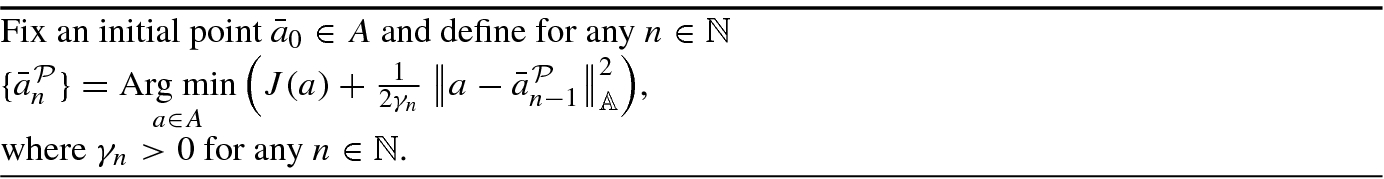
The well-definedness of algorithm (PA) and its convergence properties are recalled in the following well-known result stated in [99].

Theorem 4.5.13

Assume that the set A is compact and convex, the function J is lower semicontinuous and convex over A and $\sum _{n=1}^{+\infty }\gamma _n=+\infty$ .

Then, algorithm (PA) is well-defined and the sequence $(\bar a^{\mathcal {P}}_n)_n$ is convergent to a solution of problem (P), that is

$\displaystyle \begin{aligned} \lim_{n\to +\infty}\bar a^{\mathcal{P}}_n \in\operatorname*{\mathit{\mbox{Arg min}}}_{a\in A} J(a). \end{aligned}$

△

Remark 4.5.14

We point out that algorithm (PA) and its denomination rely on the Moreau–Yosida regularization of J with parameter γ > 0, which is the function $J_{\gamma }^{\mathcal {P}}\colon A\to [-\infty ,+\infty ]$ defined on A by

$\displaystyle \begin{aligned} J_{\gamma}^{\mathcal{P}}(a)=\inf_{x\in A}\left(J(x)+\frac{1}{2\gamma} \left\lVert {x-a} \right\rVert ^2_{\mathbb{A}}\right), \end{aligned}$

introduced previously by Moreau in [90], and also called Moreau envelope or proximal approximation. △

Therefore, the proximal point algorithm allows to approximate a solution of a convex minimization problem by constructing recursively a sequence of proximal-perturbed problems, namely

$\displaystyle \begin{aligned} (P)^{\mathcal{P}}_{\gamma_n}\colon \min_{a\in A}\left(J(a)+\frac{1}{2\gamma_{n}} \left\lVert {a-\bar a^{\mathcal{P}}_{n-1}} \right\rVert ^2_{\mathbb{A}}\right), \end{aligned}$

in general better-behaved than the original problem and that have a unique solution. Looking at the differences with respect to the Tikhonov approach, we have

the proximal-regularized problems $(P)^{\mathcal {P}}_{\gamma _n}$ are recursively defined, differently from the Tikhonov-regularized problems ${(P)^{\mathcal T}_{\lambda _n}}$ in Sect. 4.5.1.1;
the limit of the sequence generated by (PA) is “just” a minimizer of J over A, while in the Tikhonov approach the limit point is characterized as the minimum norm element in the set of minimizers of J over A;
as regards to the assumptions ensuring the convergence of algorithm (PA) and of Tikhonov method, the hypothesis on the sequence of parameters (γ _n)_n in Theorem 4.5.13 is weaker than the corresponding hypothesis on (λ _n)_n in Theorem 4.5.1.

In a one-stage games framework, we mention that algorithm (PA) has been used in [86, 99] also for approximating saddle-points in zero-sum games and in [38] in general N-player games. More recently, in [5] an alternating proximal minimization algorithm has been proposed for two-player weighted potential games and in [17] Moreau–Yosida regularization has been exploited to define a new equilibrium concept to model strategic uncertainty among players.

4.5.2.2 Proximal Regularization of the Follower’s Payoff Function in Stackelberg Games

Let Γ = (X, Y, L, F) be a Stackelberg game. We first display some preliminarily results on employing proximal regularization only in the second-stage problem similarly as presented in Sect. 4.4.1.2 for the Tikhonov regularization. We do this in order to make easier to illustrate the methodology for selecting an SPNE of Γ we will use in the next subsection which involves the regularization of both players’ payoff functions. Consider the following approach: fixed an initial point $\bar y_0\in Y$ , define for any $n\in \mathbb {N}$

$\displaystyle \begin{aligned} \{\bar\varphi^{\mathcal{P}}_n(x)\}=\operatorname*{\mbox{Arg min}}_{y\in Y}\left(F(x,y)+\frac{1}{2\gamma_{n}} \left\lVert {y-\bar\varphi^{\mathcal{P}}_{n-1}(x)} \right\rVert ^2_{\mathbb{Y}}\right)\quad \text{for any }x\in X, \end{aligned}$

(4.5.4)

where γ _n > 0 for any $n\in \mathbb {N}$ and $\bar \varphi ^{\mathcal {P}}_0(x)=\bar y_0$ for any x ∈ X.

Remark 4.5.15

Assume that Y is compact and convex, the function F is continuous over X × Y , the function F(x, ⋅) is convex over Y for any x ∈ X and $\sum _{n=1}^{+\infty }\gamma _n=+\infty$ . From Theorem 4.5.13 it straightforwardly follows that, for any x ∈ X, the sequence $(\bar \varphi ^{\mathcal {P}}_n(x))_n$ is well-defined and $\lim _{n\to +\infty }\bar \varphi ^{\mathcal {P}}_n(x)\in M(x)$ . △

Therefore, we can approach the follower’s problem (P _x) via a sequence of proximal-regularized second-stage problems recursively defined by

$\displaystyle \begin{aligned} (P_x)^{\mathcal{P}}_{\gamma_n}\colon \operatorname*{\mbox{Arg min}}_{y\in Y}\left(F(x,y)+\frac{1}{2\gamma_{n}} \left\lVert {y- \bar\varphi^{\mathcal{P}}_{n-1} (x)} \right\rVert ^2_{\mathbb{Y}}\right), \end{aligned}$

and consequently we can define the following proximal-regularized bilevel problems:

$\displaystyle \begin{aligned} (SP)^{\mathcal P}_{\gamma_n} \,\begin{cases} \underset{x\in X}{\min}\,\,L(x,\bar\varphi^{\mathcal{P}}_n(x)) \\ \text{where } \bar\varphi^{\mathcal{P}}_n(x)\text{ is the solution to } {{(P_x)^{\mathcal{P}}_{\gamma_n}}} \end{cases} \end{aligned}$

which come out to be Stackelberg problems, since the solution to the second-stage problem of ${(SP)^{\mathcal {P}}_{\gamma _n}}$ is unique for any $n\in \mathbb {N}$ . Analogously to Sect. 4.5.1.2, we are interested in two questions.

1.
Are there solutions to ${(SP)^{\mathcal {P}}_{\gamma _n}}$ ?
2.
What happens when n → +∞?

By means of the maximum theorem, the function $\bar \varphi ^{\mathcal {P}}_n\colon X\to Y$ defined in (4.5.4) is continuous over X, so the next proposition provides the answer to the first question.

Proposition 4.5.16

Assume that the set X is compact, Y is compact and convex, the functions L and F are continuous over X × Y and the function F(x, ⋅) is convex over Y for any x ∈ X.

Then, the proximal-regularized Stackelberg problem ${(SP)^{\mathcal {P}}_{\gamma _n}}$ has at least one solution, for any $n\in \mathbb {N}$ . △

Concerning the second question, the limit of the sequence generated by the solutions to ${(SP)^{\mathcal {P}}_{\gamma _n}}$ for any $n\in \mathbb {N}$ has no connections, in general, either with weak Stackelberg (or pessimistic) solutions to (PB) or with strong Stackelberg (or optimistic) solutions to (OB), as illustrated in the following example also used in [22].

The Sequence of Solutions to ${(SP)^{\mathcal {P}}_{\gamma _n}}$ May Not Converge to Weak or to Strong Stackelberg Solutions

Consider X = [1∕2, 2], Y = [−1, 1],

$\displaystyle \begin{aligned} L(x,y)=x+y\quad \text{and}\quad F(x,y)=\begin{cases} 0, & \mbox{if } x\in[1/2,1[ \\ (x-1)y, & \mbox{if } x\in [1,2]. \end{cases} \end{aligned}$

Choosing $\bar y_0=1$ and γ _n = n, we obtain

$\displaystyle \begin{aligned} \bar\varphi^{\mathcal{P}}_n(x)=\begin{cases} 1, & \mbox{if } x\in [{1}/{2},1] \\ c_n-c_nx+1, & \mbox{if } x\in ]1,1+{2}/{c_n}] \\ -1, & \mbox{if } x\in ]1+{2}/{c_n},2], \end{cases} \end{aligned}$

where the sequence (c _n)_n is recursively defined by c ₁ = 1 and c _n+1 = c _n + n + 1 for any n ≥ 1.

Hence, the solution to ${(SP)^{\mathcal {P}}_{\gamma _n}}$ is

$\displaystyle \begin{aligned} \bar u^{\mathcal{P}}_n=\begin{cases} {1}/{2}, & \mbox{if } n=1 \\ 1+{2}/{c_n}, & \mbox{if } n\geq 2. \end{cases} \end{aligned}$

Since lim_n→+∞c _n = +∞, the sequence $(\bar u^{\mathcal {P}}_n)_n$ converges to 1, which is neither a weak nor a strong Stackelberg solution. In fact, a solution to (PB) does not exist, whereas the solution to (OB) is 1∕2. Consequently, even the sequence $(\bar u^{\mathcal {P}}_n,\bar \varphi ^{\mathcal {P}}_n(\bar u^{\mathcal {P}}_n))_n$ does not converge either to a weak or to a strong Stackelberg equilibrium.

Example above shows also that, in general, the sequence of functions $(\bar \varphi ^{\mathcal {P}}_n)_n$ is not continuously convergent. In fact, coming back to such an example, it is sufficient to note that the pointwise limit of $(\bar \varphi ^{\mathcal {P}}_n)_n$ defined by

$\displaystyle \begin{aligned} \lim_{n\to+\infty}\bar\varphi^{\mathcal{P}}_n(x)=\begin{cases} 1, & \mbox{if } x\in[1/2,1] \\ -1, & \mbox{if } x\in ]1,2], \end{cases} \end{aligned}$

is not a continuous function.

We mention that methods involving proximal regularization have been recently proposed in [100, 102] for solving the simple bilevel optimization problem

$\displaystyle \begin{aligned} (SBP) \,\begin{cases} \underset{x\in E}{\min}\,\,l(x) \\ \text{where }{E}=\underset{x\in \Delta}{\operatorname*{\mbox{Arg min}}}\,\,f(x), \end{cases} \end{aligned}$

with Δ convex subset of $\mathbb {R}^n$ and l and f real-valued convex functions defined on $\mathbb {R}^n$ . Such a problem, firstly studied in [106] and labelled as “simple” in [30], involves a non-parametric second-stage problem differently from the general definitions of (PB) and (OB), and its solutions clearly coincide with the weak and strong Stackelberg solutions. Consequently, problem (SBP) does not entail the same kind of inherent difficulties that bilevel optimization problems (PB) and (OB) exhibit regarding the regularization issue, as illustrated in this subsection and in Sect. 4.5.1.2.

4.5.2.3 Selection of SPNEs via Proximal Regularization

Let us present now how proximal regularization has been employed in Stackelberg games in order to select SPNEs. Caruso, Ceparano and Morgan introduced in [22] a behavioural motivated constructive method which involves the proximal regularization both in the second-stage and in the first-stage problem (the additional regularization of the leader’s payoff function has been done in order to strongly motivate the behavioural interpretation of the method). Anyway, if the proximal regularization is carried out only in the second-stage problem, by arguing analogously as in the proofs in [22], a selection result for SPNEs can be proved even in such a case.

Let Γ = (X, Y, L, F) be a Stackelberg game and consider the following procedure.

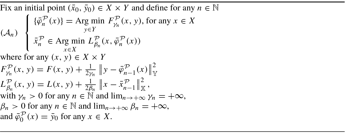
Stackelberg game proximal procedure (SGP)

../images/480569_1_En_4_Chapter/480569_1_En_4_Figb_HTML.png

Procedure (SGP) allows to construct recursively a sequence of strategies $(\bar \varphi ^{\mathcal {P}}_n(\cdot ))_n$ , where $\bar \varphi ^{\mathcal {P}}_n$ is a function from X to Y , and a sequence of leader’s actions $(\bar x^{\mathcal {P}}_n)_n$ , where $\bar x^{\mathcal {P}}_n\in X$ . We point out that looking only at the follower’s stage in procedure (SGP), one can recognize the same approach illustrated in Sect. 4.5.2.2 (for this reason here we kept unchanged the notation $\bar \varphi ^{\mathcal {P}}_n$ used previously).

In the next proposition, the well-definedness of procedure (SGP) and its regularity and convergence properties are stated.

Proposition 4.5.17 ([22, Prop. 1 and 2])

Under the assumptions of Proposition 4.5.16we have

procedure (SGP) is well-defined;
for any sequence (x _k)_kconverging to x in X, we have
$\displaystyle \begin{aligned} \lim_{k\to +\infty}\bar\varphi^{\mathcal{P}}_n(x_k)=\bar\varphi^{\mathcal{P}}_n(x)\quad \mathit{\text{for any }}n\in \mathbb{N}; \end{aligned}$
for any x ∈ X the sequence $(\bar \varphi ^{\mathcal {P}}_n(x))_n$ is convergent in Y to a solution of problem (P _x).△

Thanks to the well-definedness of procedure (SGP), we can construct recursively a sequence of proximal-regularized Stackelberg games $(\Gamma ^{\mathcal P}_{\upsilon _n})_n$ where

$\displaystyle \begin{aligned} \Gamma^{\mathcal P}_{\upsilon_n}=(X,Y,L^{\mathcal{P}}_{\beta_n},F^{\mathcal{P}}_{\gamma_n}) \end{aligned}$

is the game obtained from Γ by replacing the players’ payoff functions L and F with the proximal-regularized functions $L^{\mathcal {P}}_{\beta _n}$ and $F^{\mathcal {P}}_{\gamma _n}$ and υ _n = (β _n, γ _n). Then, Proposition 4.5.17 shows in particular that for any $n\in \mathbb {N}$ the follower’s best reply correspondence in $\Gamma ^{\mathcal P}_{\upsilon _n}$ is single-valued and that the strategy profile $(\bar x^{\mathcal {P}}_n,\bar \varphi ^{\mathcal {P}}_n(\cdot ))\in X\times Y^X$ generated at step $(\mathcal {A}_n)$ of procedure (SGP) is an SPNE of $\Gamma ^{\mathcal P}_{\upsilon _n}$ obtained as update of $(\bar x^{\mathcal {P}}_{n-1},\bar \varphi ^{\mathcal {P}}_{n-1}(\cdot ))$ , SPNE of $\Gamma ^{\mathcal P}_{\upsilon _{n-1}}$ .

Before stating the SPNE selection result, we highlight that procedure (SGP) has a behavioural interpretation linked to the costs that players face when deviating from their current actions, which is presented below.

Interpretation of the Procedure

At the generic step $(\mathcal A_n)$ of procedure (SGP), the follower chooses his strategy $\bar \varphi ^{\mathcal {P}}_n$ taking into account his previous strategy $\bar \varphi ^{\mathcal {P}}_{n-1}$ . In making such a choice, he finds an action that compromises between minimizing F(x, ⋅) and being near to $\bar \varphi ^{\mathcal {P}}_{n-1}(x)$ , for any x ∈ X. The latter purpose is motivated according to an anchoring effect, explained in [5, Subsection 1.4], which is formulated by adding a quadratic slight cost to move that reflects the difficulty of changing the previous action. The coefficient γ _n is linked to the per unit of distance cost to move of the follower and it is related to the trade-off parameter between minimizing F(x, ⋅) and minimizing the distance from $\bar \varphi ^{\mathcal {P}}_{n-1}(x)$ . Since the same arguments apply for the preceding steps until going up to step $(\mathcal A_1)$ , it follows that $\bar \varphi ^{\mathcal {P}}_n(x)$ as well as the limit of $\bar \varphi ^{\mathcal {P}}_n(x)$ embed the willingness of being near to $\bar y_0$ . Analogous observations hold also for the leader, who chooses an action having in mind to be near to his previous choices, and therefore even with the purpose of being near to $\bar x_0$ .

By taking into account the limit of the sequence of action profiles $(\bar x^{\mathcal {P}}_n,\bar \varphi ^{\mathcal {P}}_n(\bar x^{\mathcal {P}}_n))_n$ , the following existence result of an SPNE’s selection holds.

Theorem 4.5.18 ([22, Th. 1])

Assume that hypotheses of Proposition 4.5.16are satisfied and let $(\bar x^{\mathcal {P}}_n,\bar \varphi ^{\mathcal {P}}_n(\cdot ))_n$ be the sequence of strategy profiles generated by procedure (SGP).

If the sequence $(\bar x^{\mathcal {P}}_n,\bar \varphi ^{\mathcal {P}}_n(\bar x^{\mathcal {P}}_n))_n$ converges to $(\bar x^{\mathcal {P}},\bar y^{\mathcal {P}})$ in X × Y , then the strategy profile $(\bar x^{\mathcal {P}},\widetilde \varphi ^{\mathcal {P}}(\cdot ))$ where

$\displaystyle \begin{aligned} \widetilde\varphi^{\mathcal{P}}(x)=\begin{cases} \bar y^{\mathcal{P}}, & \mathit{\mbox{if }} x=\bar x^{\mathcal{P}} \\ \underset{n\to +\infty}{\lim}\,\,\bar\varphi^{\mathcal{P}}_n(x), & \mathit{\mbox{if }} x\neq\bar x^{\mathcal{P}}, \end{cases} \end{aligned}$

is an SPNE of Γ. △

Theorem 4.5.18 points out that the sequence $(\bar x^{\mathcal {P}}_n,\bar \varphi ^{\mathcal {P}}_n(\cdot ))_n$ of SPNEs of the proximal-regularized games $(\Gamma ^{\mathcal P}_{\upsilon _n})_n$ could not converge to an SPNE of Γ. This happens because the follower’s strategy $\widetilde \varphi ^{\mathcal {P}}$ in the SPNE defined according to Theorem 4.5.18 could differ from the pointwise limit, whose existence is ensured by Proposition 4.5.17, of sequence $(\bar \varphi ^{\mathcal {P}}_n)_n$ in one point. In fact, denoted with $\bar \varphi \colon X\to Y$ such a pointwise limit, if the two limits

$\displaystyle \begin{aligned} \lim_{n\to+\infty}{\bar\varphi^{\mathcal{P}}_n(\bar x^{\mathcal{P}}_n)}\quad \text{and}\quad \lim_{n\to+\infty}{\bar\varphi^{\mathcal{P}}_n(\bar x^{\mathcal{P}})}, \end{aligned}$

(4.5.5)

where $\bar x^{\mathcal {P}}=\lim _{n\to +\infty }\bar x^{\mathcal {P}}_n$ , coincide, then $\widetilde \varphi ^{\mathcal {P}}(x)=\bar \varphi (x)$ for any x ∈ X and the strategy profile $(\bar x^{\mathcal {P}},\bar \varphi )$ is an SPNE of Γ in light of Theorem 4.5.18. Instead, if the two limits in (4.5.5) do not coincide, then $\widetilde \varphi ^{\mathcal {P}}(\bar x^{\mathcal {P}})\neq \bar \varphi (\bar x^{\mathcal {P}})$ and the strategy profile $(\bar x^{\mathcal {P}},\bar \varphi )$ could be not an SPNE of Γ, hence we need the follower’s strategy $\widetilde \varphi ^{\mathcal {P}}$ as in statement of Theorem 4.5.18 in order to get an SPNE. Examples 2 and 3 in [22] illustrate the two cases described above: in the first one the two limits in (4.5.5) are equal, whereas, in the second one the two limits in (4.5.5) are different and the pair $(\bar x^{\mathcal {P}},\bar \varphi )$ comes out to be not an SPNE of the game. Such examples show also that, in general, the sequence $(\bar \varphi ^{\mathcal {P}}_n)_n$ is not continuously convergent to $\bar \varphi$ .

As regards to the connections with other methods for selecting SPNEs, the following example (examples 3, 5 and 6 in [22]) shows that the selection method based on proximal regularization presented in this subsection, the selection method relying on Tikhonov regularization described in Sect. 4.5.1.3 and the way of selecting via weak and strong Stackelberg solutions illustrated in Remark 4.3.5 do not generate, in general, the same SPNE.

The Considered Selection Methods May Select All Different SPNEs

Consider X, Y , L and F defined as in the example on page 51. We have that

the SPNE selected via proximal regularization is $(1,\widetilde \varphi ^{\mathcal {P}})$ , where
$\displaystyle \begin{aligned} \widetilde\varphi^{\mathcal{P}}(x)=\begin{cases} 1, & \mbox{if } x \in\left[{1}/{2},1\right[ \\ -1, & \mbox{if } x\in[1,2]; \end{cases} \end{aligned}$
the SPNE selected by using the Tikhonov regularization is $(1,\widetilde \varphi ^{\mathcal {T}})$ , where
$\displaystyle \begin{aligned} \widetilde\varphi^{\mathcal{T}}(x)=\begin{cases} 0, & \mbox{if } x\in[1/2,1[ \\ -1, & \mbox{if } x\in[1,2]; \end{cases} \end{aligned}$
there are no SPNEs induced by a weak Stackelberg solution, as problem (PB) has no solutions;
there exists one SPNE induced by the (unique) strong Stackelberg solution: the pair $(1/2,\bar \psi )$ where $\bar \psi (x)=-1$ for any x ∈ [1∕2, 2].

Finally, we mention that convergence results involving “costs of change” and proximal methods in Stackelberg games have been recently investigated in [37, Section 5].

4.6 Conclusion

In this chapter we considered two-stage Stackelberg games, the natural environment for different kinds of mathematical problems that can arise depending on the leader’s information about the optimal responses of the follower. We discussed crucial issues related to such problems and we provided two approaches for managing them. The first one consists in regularizing the follower’s optimal reaction set via the introduction of appropriate solution concepts which allowed to obviate both the lack of existence and stability of the weak Stackelberg (or pessimistic bilevel) problem and the lack of stability of the strong Stackelberg (or optimistic bilevel) problem. The second one consists in regularizing the follower’s payoff function by employing the Tikhonov and the proximal regularizations which enabled both to overcome the non-single-valuedness of the follower’s best reply correspondence and to select subgame perfect Nash equilibria.

We note that the issues and the approaches (for facing such issues) we focused in this chapter are not the unique ones. For instance, the question of sensitivity analysis for problems (PB) and (OB), has been recently investigated in [31, 32]. Moreover, beyond the two regularizing approaches examined in this chapter, one can construct classes of mixed regularization methods which exploit simultaneously both the idea of regularizing the follower’s optimal reaction set and of regularizing the follower’s payoff function; first approximation schemes of this type have been defined in [75, 78, 88].

For the sake of brevity, we dealt with Stackelberg games only in a static framework (that is any player has actions which do not evolve over time) where players have a single objective and just one leader acts in the first stage. However, such a Stackelberg game model has been extended in many directions:

Dynamic: players’ actions are functions depending on time. First results on dynamic Stackelberg games can be found in [10, 20, 24, 68, 105, 110], while applications to economic models are described in [11, 33].
Multiobjective: the follower has a vector-valued payoff function or solves vector (quasi-)variational inequalities. Methods for solving (optimistic) multiobjective bilevel optimization problems have been investigated in [35] (where scalarization techniques are used) and in [113] (where a model based on set-valued optimization is firstly proposed to manage strong Stackelberg problems and then extended to a multiobjective setting). Concerning results on approximate solutions which could be useful in the analysis of Stackelberg games with second stage described by vector problems, we remind [56, 65, 79, 92]. Furthermore, a penalty scheme has been introduced to approach (optimistic) semivectorial bilevel optimization problems in [18] and, in a dynamic framework, existence results have been first obtained for the (optimistic and pessimistic) semivectorial bilevel optimal control problems in [19].
Multileader: more than one leader acts in the first stage. For general multi-leader-follower games see, for example, [42, 98]. The situation where each follower can observe the action of one leader has been investigated in [97] for an economic model and in [23] for deriving a selection result. An increasing literature is also devoted to the class of multi-leader-common-follower games and to its applications to electricity markets, see for example [8, 9].

We emphasize that for the situations illustrated above it would be interesting to provide new concepts and results which derive from the analogous exploitation of the two types of regularization approaches presented in the chapter.

References

1.
A. Aboussoror, P. Loridan, Strong-weak Stackelberg problems in finite dimensional spaces. Serdica Math. J. 21, 151–170 (1995). http://www.math.bas.bg/serdica/n2_95.html
2.
A. Aboussoror, P. Loridan, Existence of solutions to two-level optimization problems with nonunique lower-level solutions. J. Math. Anal. Appl. 254, 348–357 (2001). https://doi.org/10.1006/jmaa.2000.7001
3.
A. Aboussoror, A. Mansouri, Weak linear bilevel programming problems: existence of solutions via a penalty method. J. Math. Anal. Appl. 304, 399–408 (2005). https://doi.org/10.1016/j.jmaa.2004.09.033
4.
A. Aboussoror, S. Adly, F.E. Saissi, Strong-weak nonlinear bilevel problems: existence of solutions in a sequential setting. Set-Valued Var. Anal. 25, 113–132 (2017). https://doi.org/10.1007/s11228-016-0369-4
5.
H. Attouch, P. Redont, A. Soubeyran, A new class of alternating proximal minimization algorithms with costs-to-move. SIAM J. Optim. 18, 1061–1081 (2007). https://doi.org/10.1137/060657248
6.
J.-P. Aubin, H. Frankowska, Set-Valued Analysis (Birhäuser, Boston, 1990)
7.
A. Auslender, Recherche des points de selle d’une fonction, in Symposium on Optimization, ed. by A.V. Balakrishnan, M. Contensou, B.F. de Veubeke, P. Krée, J.L. Lions, N.N. Moiseev (Springer, Berlin, 1970), pp. 37–52. https://doi.org/10.1007/BFb0066671
8.
D. Aussel, P. Bendotti, M. Pištěk, Nash equilibrium in a pay-as-bid electricity market: part 1—existence and characterization. Optimization 66, 1013–1025 (2017). https://doi.org/10.1080/02331934.2016.1227981
9.
D. Aussel, P. Bendotti, M. Pištěk, Nash equilibrium in a pay-as-bid electricity market: part 2—best response of a producer. Optimization 66, 1027–1053 (2017). https://doi.org/10.1080/02331934.2016.1227982
10.
T. Başar, G. Olsder, Dynamic Noncooperative Game Theory (Society for Industrial and Applied Mathematics, Philadelphia, 1998)
11.
A. Bagchi, Stackelberg Differential Games in Economic Models. Lecture Notes in Control and Information Sciences, vol. 64 (Springer, Berlin, 1984)
12.
C. Baiocchi, A. Capelo, Variational and Quasi-Variational Inequalities (John Wiley and Sons, New York, 1984)
13.
B. Bank, J. Guddat, D. Klatte, B. Kummer, K. Tammer, Non-Linear Parametric Optimization (Birkhäuser, Basel, 1983)
14.
J.F. Bard, An algorithm for solving the general bilevel programming problem. Math. Oper. Res. 8, 260–272 (1983). https://doi.org/10.1287/moor.8.2.260
15.
J.F. Bard, J.E. Falk, An explicit solution to the multi-level programming problem. Comput. Oper. Res. 9, 77–100 (1982). https://doi.org/10.1016/0305-0548(82)90007-7
16.
C. Berge, Espaces topologiques et fonctions multivoques (Dunod, 1959) [Translation: E.M. Patterson. Topological Spaces) (Oliver & Boyd, 1963)]
17.
P. Bich, Strategic uncertainty and equilibrium selection in discontinuous games. J. Econ. Theory 183, 786–822 (2019). https://doi.org/10.1016/j.jet.2019.08.001
18.
H. Bonnel, J. Morgan, Semivectorial bilevel optimization problem: penalty approach. J. Optim. Theory Appl. 131, 365–382 (2006). https://doi.org/10.1007/s10957-006-9150-4
19.
H. Bonnel, J. Morgan, Semivectorial bilevel convex optimal control problems: existence results. SIAM J. Control Optim. 50, 3224–3241 (2012). https://doi.org/10.1137/100795450
20.
M. Breton, A. Alj, A. Haurie, Sequential Stackelberg equilibria in two-person games. J. Optim. Theory Appl. 59, 71–97 (1988). https://doi.org/10.1007/BF00939867
21.
D. Cao, L.C. Leung, A partial cooperation model for non-unique linear two-level decision problems. Eur. J. Oper. Res. 140, 134–141 (2002). https://doi.org/10.1016/S0377-2217(01)00225-9
22.
F. Caruso, M.C. Ceparano, J. Morgan, Subgame perfect Nash equilibrium: a learning approach via costs to move. Dyn. Games Appl. 9, 416–432 (2019). https://doi.org/10.1007/s13235-018-0277-3
23.
M.C. Ceparano, J. Morgan, Equilibrium selection in multi-leader-follower games with vertical information. TOP 25, 526–543 (2017). https://doi.org/10.1007/s11750-017-0444-5
24.
C. Chen, J.B. Cruz, Stackelberg solution for two-person games with biased information patterns. IEEE Trans. Autom. Control 17, 791–798 (1972). https://doi.org/10.1109/TAC.1972.1100179
25.
J.B. Clempner, A.S. Poznyak, Computing the strong Nash equilibrium for Markov chains games. Appl. Math. Comput. 265, 911–927 (2015). https://doi.org/10.1016/j.amc.2015.06.005
26.
S. Dempe, A simple algorithm for the linear bilevel programming problem. Optimization 18, 373–385 (1987). https://doi.org/10.1080/02331938708843247
27.
S. Dempe, A bundle algorithm applied to bilevel programming problems with non-unique lower level solutions. Comput. Optim. Appl. 15, 145–166 (2000). https://doi.org/10.1023/A:1008735010803
28.
S. Dempe, Foundations of Bilevel Programming (Springer, New York, 2002)
29.
S. Dempe, H. Schmidt, On an algorithm solving two-level programming problems with nonunique lower level solutions. Comput. Optim. Appl. 6, 227–249 (1996). https://doi.org/10.1007/BF00247793
30.
S. Dempe, N. Dinh, J. Dutta, Optimality conditions for a simple convex bilevel programming problem, in: Variational Analysis and Generalized Differentiation in Optimization and Control: In Honor of Boris S. Mordukhovich, ed. by R.S. Burachik, J.-C. Yao (Springer, New York, 2010), pp. 149–161. https://doi.org/10.1007/978-1-4419-0437-9_7
31.
S. Dempe, B. Mordukhovich, A.B. Zemkoho, Sensitivity analysis for two-level value functions with applications to bilevel programming. SIAM J. Optim. 22, 1309–1343 (2012). https://doi.org/10.1137/110845197
32.
S. Dempe, B.S. Mordukhovich, A.B. Zemkoho, Two-level value function approach to non-smooth optimistic and pessimistic bilevel programs. Optimization 68, 433–455 (2019). https://doi.org/10.1080/02331934.2018.1543294
33.
E.J. Dockner, S. Jorgensen, N.V. Long, G. Sorger, Differential Games in Economics and Management Science (Cambridge University Press, Cambridge, 2000)
34.
L. Drouet, A. Haurie, F. Moresino, J.-P. Vial, M. Vielle, L. Viguier, An oracle based method to compute a coupled equilibrium in a model of international climate policy. Comput. Manag. Sci. 5, 119–140 (2008). https://doi.org/10.1007/s10287-007-0043-2
35.
G. Eichfelder, Multiobjective bilevel optimization. Math. Program. 123, 419–449 (2010). https://doi.org/10.1007/s10107-008-0259-0
36.
A. Evgrafov, M. Patriksson, On the convergence of stationary sequences in topology optimization, Int. J. Numer. Methods Eng. 64, 17–44 (2005). https://doi.org/10.1002/nme.1359
37.
S.D. Flåm, On games and cost of change. Ann. Oper. Res. (2020). https://doi.org/10.1007/s10479-020-03585-w
38.
S.D. Flåm, G.H. Greco, Non-cooperative games; methods of subgradient projection and proximal point, in Advances in Optimization, ed. by W. Oettli, D. Pallaschke (Springer, Berlin, 1992), pp. 406–419. https://doi.org/10.1007/978-3-642-51682-5_27
39.
D. Fudenberg, J. Tirole, Game Theory (MIT Press, Cambridge, 1991)
40.
J.C. Harsanyi, R. Selten, A General Theory of Equilibrium Selection in Games (The MIT Press, Cambridge, 1988)
41.
A. Haurie, J.B. Krawczyk, G. Zaccour, Games and Dynamic Games (World Scientific Publishing Company, Singapore, 2012)
42.
M. Hu, M. Fukushima, Existence, uniqueness, and computation of robust Nash equilibria in a class of multi-leader-follower games. SIAM J. Optim. 23, 894–916 (2013). https://doi.org/10.1137/120863873
43.
A. Kannan, U. Shanbhag, Distributed computation of equilibria in monotone Nash games via iterative regularization techniques. SIAM J. Optim. 22 (2012), 1177–1205. https://doi.org/10.1137/110825352
44.
L. Lampariello, S. Sagratella, Numerically tractable optimistic bilevel problems. Comput. Optim. Appl. 76, 277–303 (2020). https://doi.org/10.1007/s10589-020-00178-y
45.
L. Lampariello, S. Sagratella, O. Stein, The standard pessimistic bilevel problem. SIAM J. Optim. 29, 1634–1656 (2019). https://doi.org/10.1137/18M119759X
46.
G. Leitmann, On generalized Stackelberg strategies. J. Optim. Theory Appl. 26, 637–643 (1978). https://doi.org/10.1007/BF00933155
47.
B. Lemaire, Jeux dans les equations aux derivees partielles, in, Symposium on Optimization, ed. by A.V. Balakrishnan, M. Contensou, B.F. de Veubeke, P. Krée, J.L. Lions, N.N. Moiseev (Springer, Berlin, 1970), pp. 181–195. https://doi.org/10.1007/BFb0066682
48.
M.B. Lignola, Well-posedness and l-well-posedness for quasivariational inequalities. J. Optim. Theory Appl. 128, 119–138 (2006). https://doi.org/10.1007/s10957-005-7561-2
49.
M.B. Lignola, J. Morgan, Semi-continuities of marginal functions in a sequential setting. Optimization 24, 241–252 (1992). https://doi.org/10.1080/02331939208843793
50.
M.B. Lignola, J. Morgan, Approximate solutions to variational inequalities and applications. Le Matematiche 49, 281–293 (1995). https://lematematiche.dmi.unict.it/index.php/lematematiche/article/view/528
51.
M.B. Lignola, J. Morgan, Topological existence and stability for Stackelberg problems. J. Optim. Theory Appl. 84, 145–169 (1995). https://doi.org/10.1007/BF02191740
52.
M.B. Lignola, J. Morgan, Stability of regularized bilevel programming problems. J. Optim. Theory Appl. 93, 575–596 (1997). https://doi.org/10.1023/A:1022695113803
53.
M.B. Lignola, J. Morgan, Existence of solutions to generalized bilevel programming problem, in Multilevel Optimization: Algorithms and Applications, ed. by A. Migdalas, P.M. Pardalos, P. Värbrand (Springer, Boston, 1998), pp. 315–332. https://doi.org/10.1007/978-1-4613-0307-7_14
54.
M.B. Lignola, J. Morgan, Well-posedness for optimization problems with constraints defined by variational inequalities having a unique solution. J. Glob. Optim. 16, 57–67 (2000). https://doi.org/10.1023/A:1008370910807
55.
M.B. Lignola, J. Morgan, α-well-posedness for Nash equilibria and for optimization problems with Nash equilibrium constraints. J. Glob. Optim. 36, 439–459 (2006). https://doi.org/10.1007/s10898-006-9020-5
56.
M.B. Lignola, J. Morgan, Vector quasi-variational inequalities: approximate solutions and well-posedness. J. Convex Anal. 13, 373–384 (2006). http://www.heldermann.de/JCA/JCA13/JCA132/jca13031.htm
57.
M.B. Lignola, J. Morgan, Approximate values for mathematical programs with variational inequality constraints. Comput. Optim. Appl. 53(2), 485–503 (2012). https://doi.org/10.1007/s10589-012-9470-2
58.
M.B. Lignola, J. Morgan, Stability in regularized quasi-variational settings. J. Convex Anal. 19, 1091–1107 (2012). http://www.heldermann.de/JCA/JCA19/JCA194/jca19058.htm
59.
M.B. Lignola, J. Morgan, Approximating values of minsup problems with quasi-variational inequality constraints. Pac. J. Optim. 10, 749–765 (2014). http://www.ybook.co.jp/online2/pjov10.html
60.
M.B. Lignola, J. Morgan, Viscosity solutions for bilevel problems with Nash equilibrium constraints. Far Est J. Appl. Math. 88, 15–34 (2014). http://www.pphmj.com/abstract/8683.htm
61.
M.B. Lignola, J. Morgan, Asymptotic behavior of semi-quasivariational optimistic bilevel problems in Banach spaces. J. Math. Anal. Appl. 424, 1–20 (2015). https://doi.org/10.1016/j.jmaa.2014.10.059
62.
M.B. Lignola, J. Morgan, A method to bypass the lack of solutions in minsup problems under quasi-equilibrium constraints. Optim. Lett. 10, 833–846 (2016). https://doi.org/10.1007/s11590-015-0956-6
63.
M.B. Lignola, J. Morgan, Inner regularizations and viscosity solutions for pessimistic bilevel optimization problems. J. Optim. Theory Appl. 173, 183–202 (2017). https://doi.org/10.1007/s10957-017-1085-4
64.
M.B. Lignola, J. Morgan, Further on inner regularizations in bilevel optimization. J. Optim. Theory Appl. 180, 1087–1097 (2019). https://doi.org/10.1007/s10957-018-1438-7
65.
M.B. Lignola, J Morgan, V. Scalzo, Lower convergence of approximate solutions to vector quasi-variational problems. Optimization 59, 821–832 (2010). https://doi.org/10.1080/02331930902863707
66.
G.-H. Lin, M. Xu, J.J. Ye, On solving simple bilevel programs with a nonconvex lower level program. Math. Program. 144, 277–305 (2014). https://doi.org/10.1007/s10107-013-0633-4
67.
P. Loridan, J. Morgan, Approximation results for two-level optimization problem and application to penalty methods, Preprint n.52-1985. Dipartimento di Matematica e Applicazioni R. Caccioppoli, Università di Napoli, December 1984. https://www.researchgate.net/publication/335619596_Approximation_results_for_a_two-level_optimization_problem_and_application_to_penalty_methods
68.
P. Loridan, J. Morgan, Approximation of the Stackelberg problem and applications in control theory. Annu. Rev. Autom. Program. 13, 121–124 (1985). https://doi.org/10.1016/0066-4138(85)90472-0
69.
P. Loridan, J. Morgan, Approximate solutions for two-level optimization problems, in Trends in Mathematical Optimization: 4th French-German Conference on Optimization 1986, ed. by K.-H. Hoffmann, J. Zowe, J.-B. Hiriart-Urruty, C. Lemarechal (Birkhäuser, Basel, 1988), pp. 181–196. https://doi.org/10.1007/978-3-0348-9297-1_13
70.
P. Loridan, J. Morgan, 𝜖-regularized two-level optimization problems: approximation and existence results, in Optimization: Proceedings of the Fifth French–German Conference Held in Castel-Novel (Varetz), October 3–8, 1988, ed. by S. Dolecki (Springer, Berlin, 1989), pp. 99–113. https://doi.org/10.1007/BFb0083589
71.
P. Loridan, J. Morgan, New results on approximate solution in two-level optimization. Optimization 20, 819–836 (1989). https://doi.org/10.1080/02331938908843503
72.
P. Loridan, J. Morgan, A sequential stability result for constrained Stackelberg problems. Ric. Mat. 38, 19–32 (1989). https://www.researchgate.net/publication/266591292_A_sequential_stability_result_for_constrained_Stackelberg_problems
73.
P. Loridan, J. Morgan, A theoretical approximation scheme for Stackelberg problems. J. Optim. Theory Appl. 61, 95–110 (1989). https://doi.org/10.1007/BF00940846
74.
P. Loridan, J. Morgan, Quasi convex lower level problem and applications in two level optimization, in Proceedings of the International Workshop on “Generalized Concavity, Fractional Programming and Economic Applications” Held at the University of Pisa, Italy, May 30–June 1, 1988, ed. by A. Cambini, E. Castagnoli, L. Martein, P. Mazzoleni, S. Schaible (Springer, Berlin, 1990), pp. 325–341. https://doi.org/10.1007/978-3-642-46709-7_23
75.
P. Loridan, J. Morgan, Least-norm regularization for weak two-level optimization problems, in Optimization, Optimal Control and Partial Differential Equations, ed. by V. Barbu, D. Tiba, J.F. Bonnans (Birkhäuser, Basel, 1992), pp. 307–318. https://doi.org/10.1007/978-3-0348-8625-3_28
76.
P. Loridan, J. Morgan, On strict-solution for a two level optimization problem, in Proceedings of The international Conference On Operation Research, ed. by G. Feichtinger, W. Bühler, F. Radermacher, P. Stähly (Springer Verlag, Vienna, 1992), pp. 165–172. https://doi.org/10.1007/978-3-642-77254-2_19
77.
P. Loridan, J. Morgan, Regularizations for two-level optimization problems, in Advances in Optimization, ed. by W. Oettli, D. Pallaschke (Springer, Berlin, 1992), pp. 239–255. https://doi.org/10.1007/978-3-642-51682-5_16
78.
P. Loridan, J. Morgan, Weak via strong Stackelberg problem: new results. J. Glob. Optim. 263–287 (1996). https://doi.org/10.1007/BF00121269
79.
P. Loridan, J. Morgan, Convergence of approximate solutions and values in parametric vector optimization, in Vector Variational Inequalities and Vector Equilibria: Mathematical Theories, ed. by F. Giannessi (Springer, Boston, 2000), pp. 335–350. https://doi.org/10.1007/978-1-4613-0299-5_19
80.
R. Lucchetti, F. Mignanego, G. Pieri, Existence theorems of equilibrium points in Stackelberg games with constraints. Optimization 18, 857–866 (1987). https://doi.org/10.1080/02331938708843300
81.
Z.-Q. Luo, J.-S. Pang, D. Ralph, Mathematical Programs with Equilibrium Constraints (Cambridge University Press, Cambridge, 1996)
82.
L. Mallozzi, J. Morgan, Problema di Stackelberg con risposte pesate. Atti del XIX Convegno AMASES (1995), pp. 416–425
83.
L. Mallozzi, J. Morgan, Hierarchical systems with weighted reaction set, in Nonlinear Optimization and Applications, ed. by G. Di Pillo, F. Giannessi (Springer, Boston, 1996), pp. 271–282. https://doi.org/10.1007/978-1-4899-0289-4_19
84.
L. Mallozzi, J. Morgan, Oligopolistic markets with leadership and demand functions possibly discontinuous. J. Optim. Theory Appl. 125, 393–407 (2005). https://doi.org/10.1007/s10957-004-1856-6
85.
P. Marcotte, G Savard, A note on the Pareto optimality of solutions to the linear bilevel programming problem, Comput. & Oper. Res. 18, 355–359 (1991). https://doi.org/10.1016/0305-0548(91)90096-A
86.
B. Martinet, Brève communication. régularisation d’inéquations variationnelles par approximations successives. Rev. Fr. Inform. Rech. Opér. Sér. Rouge 4, 154–158 (1970). http://www.numdam.org/item/M2AN_1970__4_3_154_0/
87.
M. Maschler, E. Solan, S. Zamir, Game Theory (Cambridge University Press, Cambridge, 2013)
88.
D.A. Molodtsov, The solution of a class of non-antagonistic games. USSR Comput. Math. Math. Phys. 16, 67–72 (1976). https://doi.org/10.1016/0041-5553(76)90042-2
89.
D.A. Molodtsov, V.V. Fedorov, Approximation of two-person games with information exchange. USSR Comput. Math. Math. Phys. 13, 123–142 (1973). https://doi.org/10.1016/0041-5553(73)90010-4
90.
J.J. Moreau, Proximité et dualité dans un espace hilbertien. Bull. Soc. Math. Fr. 93, 273–299 (1965). https://doi.org/10.24033/bsmf.1625
91.
J. Morgan, Constrained well-posed two-level optimization problems, in Nonsmooth Optimization and Related Topics, ed. by F.H. Clarke, V.F. Dem’yanov, F. Giannessi (Springer, Boston, 1989), pp. 307–325. https://doi.org/10.1007/978-1-4757-6019-4_18
92.
J. Morgan, Approximations and well-posedness in multicriteria games. Ann. Oper. Res. 137, 257–268 (2005). https://doi.org/10.1007/s10479-005-2260-9
93.
J. Morgan, F. Patrone, Stackelberg problems: subgame perfect equilibria via Tikhonov regularization, in Advances in Dynamic Games: Applications to Economics, Management Science, Engineering, and Environmental Management, ed. by A. Haurie, S. Muto, L.A. Petrosjan, T.E.S. Raghavan (Birkhäuser, Boston, 2006), pp. 209–221. https://doi.org/10.1007/0-8176-4501-2_12
94.
J. Morgan, R. Raucci, Lower semicontinuity for approximate social Nash equilibria. Int. J. Game Theory 31, 499–509 (2003). https://doi.org/10.1007/s001820300134
95.
J.F. Nash, Equilibrium points in n-person games. Proc. Natl. Acad. Sci. 36, 48–49 (1950). https://doi.org/10.1073/pnas.36.1.48
96.
J.V. Outrata, On the numerical solution of a class of Stackelberg problems. Z. Oper. Res. 34, 255–277 (1990). https://doi.org/10.1007/BF01416737
97.
M. Pagnozzi, S. Piccolo, Vertical separation with private contracts. Econ. J. 122, 173–207 (2012). https://doi.org/10.1111/j.1468-0297.2011.02471.x
98.
J.-S. Pang, M. Fukushima, Quasi-variational inequalities, generalized Nash equilibria, and multi-leader-follower games. Comput. Manag. Sci. 2, 21–56 (2005). https://doi.org/10.1007/s10287-004-0010-0
99.
R.T. Rockafellar, Monotone operators and the proximal point algorithm. SIAM J. Control Optim. 14, 877–898 (1976). https://doi.org/10.1137/0314056
100.
S. Sabach, S. Shtern, A first order method for solving convex bilevel optimization problems. SIAM J. Optim. 27, 640–660 (2017). https://doi.org/10.1137/16M105592X
101.
R. Selten, Spieltheoretische Behandlung eines Oligopolmodells mit Nachfrageträgheit, Z. Gesamte Staatswiss. 121, 301–324 (1965). https://www.jstor.org/stable/40748884
102.
Y. Shehu, P.T. Vuong, A. Zemkoho, An inertial extrapolation method for convex simple bilevel optimization. Optim Methods Softw. 1–19 (2019). https://doi.org/10.1080/10556788.2019.1619729
103.
K. Shimizu, E. Aiyoshi, A new computational method for Stackelberg and min–max problems by use of a penalty method. IEEE Trans. Autom. Control 26, 460–466 (1981). https://doi.org/10.1109/TAC.1981.1102607
104.
V.F. Sholohovich, Unstable extremal problems and geometric properties of Banach spaces. Dokl. Akad. Nauk 195, 289–291 (1970). http://www.mathnet.ru/php/archive.phtml?wshow=paper&jrnid=dan&paperid=35782&option_lang=eng
105.
M. Simaan, J.B. Cruz, On the Stackelberg strategy in nonzero-sum games. J. Optim. Theory Appl. 11, 533–555 (1973). https://doi.org/10.1007/BF00935665
106.
M. Solodov, An explicit descent method for bilevel convex optimization. J. Convex Anal. 14, 227–237 (2007). http://www.heldermann.de/JCA/JCA14/JCA142/jca14016.htm
107.
A.N. Tikhonov, Methods for the regularization of optimal control problems. Sov. Math. Dokl. 6, 761–763 (1965)
108.
L. Vicente, G. Savard, J. Júdice, Descent approaches for quadratic bilevel programming, J. Optim Theory Appl. 81, 379–399 (1994). https://doi.org/10.1007/BF02191670
109.
H. von Stackelberg, Marktform und Gleichgewicht (Verlag von Julius Springer, Berlin, 1934) [Translation: D. Bazin, R. Hill, L. Urch. Market Structure and Equilibrium (Springer, Berlin, 2011)]
110.
J.J. Ye, Necessary conditions for bilevel dynamic optimization problems. SIAM J. Control Optim. 33, 1208–1223 (1995). https://doi.org/10.1137/S0363012993249717
111.
J.J. Ye, D.L. Zhu, Optimality conditions for bilevel programming problems. Optimization 33, 9–27 (1995). https://doi.org/10.1080/02331939508844060
112.
J.J. Ye, D.L. Zhu, and Q.J. Zhu, Exact penalization and necessary optimality conditions for generalized bilevel programming problems. SIAM J. Optim. 7, 481–507 (1997). https://doi.org/10.1137/S1052623493257344
113.
A.B. Zemkoho, Solving ill-posed bilevel programs. Set-Valued Var. Anal. 24, 423–448 (2016). https://doi.org/10.1007/s11228-016-0371-x