5.1 General Overview of Bilevel Programming in Energy
The liberalization of the electricity sector and the introduction of electricity markets first emerged in the 1980s in countries like Chile, the United Kingdom, and New Zealand. Nowadays, the vast majority of all developed countries have undergone such a liberalization process, which has complicated the organization of the electricity and energy sector greatly. In regulated electricity systems, many tasks—such as expansion planning, for example—are usually carried out by a centralized planner who minimizes total cost while meeting a future demand forecast, reliability constraints, and environmental requirements identified by the government. Planning the investment and operation of such a regulated system can be regarded as stable, relatively predictable, and essentially risk-free for all entities involved.
However, under a liberalized framework, many decisions are no longer regulated but to a large extent, up to the responsibility of individual entities or private companies that act strategically and might have opposing objectives. Within the realm of strategic decision making, the hierarchy in which decisions are taken becomes extremely important. A strategic storage investor maximizing profits is not going to invest the same amount as a centralized planner that maximizes social welfare, nor will the storage facility be operated in the same way. In order to characterize this strategic behavior, bilevel models inspired by Stackelberg games become necessary and important decision-support tools in electricity and energy markets.
Bilevel models—which have first been used in the electricity sector to formulate electricity markets for example by Cardell et al. [10], Berry et al. [5], Weber and Overbye [70], Hobbs et al. [26] or Ramos et al. [56] just to name a few—allow us to represent a sequential decision-making process as opposed to single-level models where all decisions are considered to be taken simultaneously, which can be a gross simplification of reality and distort model outcomes.
In energy and electricity markets, there are numerous different applications of interesting bilevel optimization and bilevel equilibrium problems. The purpose of this chapter is to provide a general overview of the areas in energy and electricity markets where bilevel programming is being used in a meaningful way. Hence, the remainder of this chapter is organized as follows. Section 5.1 contains a detailed literature review of bilevel applications in energy. Sections 5.2 and 5.3 give a brief outlook on existing solution techniques and pending challenges in bilevel models in the power sector. In Sect. 5.4 , we formulate a bilevel model that takes strategic investment decisions and compare it to a traditional model in a numerical case study. Finally, Sect. 5.5 concludes the chapter.
Section 5.1 provides a detailed but not exhaustive literature review on many different applications of bilevel programming in energy and electricity markets. We first identify several important areas to which bilevel optimization is applied: Transmission Expansion Planning, Generation Expansion Planning (conventional and renewable), Energy Storage Systems, Strategic Bidding, Natural Gas Markets, and Others. In the remainder of this section, we analyze each of those areas separately and point out what type of bilevel games can be encountered in the literature. Please note that these areas are not necessarily mutually exclusive. Therefore, relevant references might appear more than once if applicable.
5.1.1 Transmission Expansion Planning
At the core of every multi-level optimization or equilibrium problem, there lies a sequential decision-making process. When it comes to transmission expansion planning (TEP) in liberalized electricity markets, the main factor of decision hierarchy stems from the generation expansion planning (GEP). Does the transmission planner take its decisions after the generation has been decided and sited, or do generation companies plan their investments after transmission assets have been decided? What comes first, the chicken or the egg? The sequence of TEP versus GEP defines two different philosophies: proactive TEP; and, reactive TEP.
Under proactive TEP approaches, the transmission company (TRANSCO) is the Stackelberg leader, whereas generation companies (GENCOs) are the Stackelberg followers. This means that TRANSCO has the first-mover advantage and decides the best possible TEP taking into account the feedback from generation companies. In other words, the network planner can influence generation investment and, furthermore, the spot market behavior. Note that while the market operation is an essential part of TEP and GEP problems, and corresponding modeling details have to be discussed in order to establish possible gaps in the literature, in terms of decision-making sequence, market decisions happen after both GEP and TEP. Hence, the market is not the main focus in the bilevel TEP/GEP discussion.
On the other hand, under a reactive TEP approach, the network planner assumes that generation capacities are given (GENCOs are Stackelberg leaders), and then the network planner optimizes transmission expansion based only on the subsequent market operation. Reactive planning is thus represented by a model with multi-leader GENCOs and one or several TRANSCOs as followers.
Additionally, there exist some alternative TEP approaches, such as [30], where the upper level represents both GEP and TEP simultaneously, while the lower level represents the market operation (MO). In [3], the authors decide optimal wind and transmission expansion in the upper level, subject to a market-clearing. Such an approach is more suitable for a centralized power system where the network planner and the generation companies belong to the same decision-making agent. This is usually not the case in liberalized electricity markets. The work of [57] explores the interactions between an ISO with the security of supply objectives with private profit-maximizing entities deciding GEP and TEP investment simultaneously. The entire problem, however, is never explicitly formulated as a bilevel problem. Instead, an iterative solution procedure is proposed. Since our main focus lies in the sequence between TEP and GEP, we continue our detailed literature review on bilevel TEP problems distinguishing between proactive and reactive approaches.
In practice [65], most of the TRANSCOs in the world follow a reactive TEP approach, but most of the TEP-GEP literature is on proactive planning. However, Pozo et al. [54] mention other approaches that are close to proactive planning. For example, a regulation was approved in the US that includes the concept of anticipative (proactive) transmission planning to obtain a higher social welfare [20]. Additionally, in the current European context, ENTSOE plays the role of a centralized agent that proposes future planning pathways, in which regional coordination takes place, and then nationally, generation companies can react to its decisions. Thus, under this regulatory context, a proactive planning approach would make more sense.
5.1.1.1 Proactive Transmission Expansion Planning
Sauma and Oren [61] present the first work on proactive TEP we want to discuss. In [61], the authors extend their work in [60] and explore optimal transmission expansion given different objectives. They also consider a spot market where the distinctive ownership structures are reflected, as proposed in [78]. The authors consider a three-level structure: first TEP, then GEP, and finally, the market. The market equilibrium and strategic GEP already yield an equilibrium problem with equilibrium constraints (EPEC). An additional layer of TEP is set on top of that.
Pozo et al. [52] extend the groundwork of [60, 61], and propose a first complete model formulation of the three-level TEP problem. The three levels are still: first TEP, then GEP, and finally, the market-clearing. In the second level (the GEP stage), all GENCOs’ investment strategies are enumerated, expressing Nash equilibria as a set of inequalities. While this work represents a significant step forward in terms of actually formulating a three-level problem in closed form, the proposed model does not seem to be computationally efficient.
Pozo et al. [53] extend their work of [52] by including uncertainty in the demand, and apply the model to a realistic power system in Chile. The same authors overcome the computational shortcoming of their previously proposed models in [54] by proposing a novel column-and-row decomposition technique for solving the arising EPECs, which ultimately yields the global optimum. Furthermore, the authors propose a pessimistic and optimistic network planner to describe all possible outcomes of the EPEC. The authors conclude that in practice, if multiple generation expansion exists in the equilibrium, proactive planning does not always yield the best welfare results, and it can even reduce social welfare.
Jin and Ryan [31] also propose a three-level TEP problem, but they extend previous approaches by considering Cournot’s strategic decisions in the market. They propose a hybrid approach to solve the three-level problem, which proves computationally efficient; however, it does not guarantee to find the global optimum.
Motamedi et al. [42] present another multi-level approach to TEP. The authors characterize their problem as a four-level problem; however, since two of those levels refer to problems that are considered simultaneously, mathematically speaking, the framework boils down to a three-level problem: TEP, GEP, and market (pairs of price and quantity bids). The authors propose an iterative algorithm using search-based techniques and agent-based modeling to solve the arising problem.
In Taheri et al. [67], the authors also tackle a three-level TEP problem: TEP, GEP, and market clearing through price and offer quantities. The temporal representation of this work resorts to a load duration curve, which does not allow for modeling intertemporal constraints such as ramping or commitment constraints.
Apart from the three-level proactive approaches mentioned above, there are two-level approaches where transmission investment decisions are taken first, and then generation investment and operation decisions are taken simultaneously. On the one hand, the work in [29] models the perfectly competitive market clearing in the lower level, which includes GEP investment variables as well. Additionally, they consider a network fee so the TRANSCO can recover investments in the case of a flow-based fee regulation typically used in the US. The authors linearize the arising MPEC using [22] and solve it as a mixed-integer linear program (MILP)—a method frequently used in bilevel energy applications.
Pisciella et al. [51] also present a proactive TEP approach where the TSO takes investment decisions subject to a lower level market equilibrium of GENCOs and a market operator that exchange price and quantity bids and a market-clearing.
Later, Weibelzahl and Märtz [71] extend the work of Jenabi and Fatemi Ghomi [29] and choose a pessimistic TRANSCO. The authors prove some subsequent uniqueness properties. Since their model uses chronological time steps, they additionally consider battery expansion in their framework. In [69], the authors present various types of TEP-GEP models, one of which represents a proactive approach with a pessimistic TEP in the upper level, and strategic GENCOs in the lower level. On the other hand, Maurovich et al. [39] consider a stochastic bilevel model with a merchant investor of transmission in the upper level, and GEP including wind expansion and a Cournot market in the lower level.
Finally, Gonzalez-Romero et al. [23] apply the same structure, but they consider storage expansion and Cournot competition in the lower level. Both works [23, 39] find counterintuitive results when considering Cournot competition in the lower level compared to a perfect competition case.
5.1.1.2 Reactive Transmission Expansion Planning
One of the first reactive TEP approaches was proposed in [61], showing some theoretical results and some practical results for fixed transmission plans. Unfortunately, the subsequent research on this regard is limited. In general, under this approach, several GENCOs are considered as the leaders and a single TRANSCO as a follower. However, it could also be the case that only one GENCO is the leader, and the remaining GENCOs and TRANSCO(s) are followers, yielding a one leader multiple followers structure which is easier to solve numerically speaking.
In [69], Tohidi and Hesamzadeh propose a comparison between the proactive and the reactive approach. In contrast to [53], authors in [69] do not consider anticipation of market outcomes by GENCOs and propose the elimination of the multiple Nash equilibria by considering a pessimistic or optimistic TRANSCO.
Dvorkin et al. [17] present a reactive TEP with three levels: upper level representing a merchant storage owner; middle level that carries out centralized TEP; and, a lower level simulating the market-clearing, to our best knowledge mathematically speaking this is not a three-level structure as the middle (TEP), and the lower (market) level are solved simultaneously. Mathematically speaking, this belongs to the bilevel structures when merchant investors are in the upper level, and then TEP and market decisions are taken simultaneously in the lower level. The arising problem is solved numerically efficiently using a column generation algorithm, which is applied to a real-size case study. The authors conclude that the co-planning of storage and transmission leads to more significant cost savings than independent planning.
5.1.2 Generation Expansion Planning
Generation expansion planning (GEP), in general, refers to the expansion of thermal, renewable, or storage generation capacity in a power system. As we have discussed in the previous Sect. 5.1.1, many bilevel TEP problems include GEP in some way or another. In this section, however, we focus on expansion planning problems that do not include network expansion. Moreover, we also omit the discussion of the literature regarding storage investment, as this is discussed in detail in Sect. 5.1.3.
The emphasis on [11, 73] is on a single strategic generation company (GENCO) that maximizes total profits deciding generation capacity investment in conventional thermal technologies, subject to a strategic market equilibrium using conjectural variations. The use of conjectural variations allows the authors to emulate different degrees of strategic market behavior, ranging from perfect competition to the Cournot oligopoly. The market equilibrium is obtained as the system of KKT conditions of all market players, i.e., also the GENCOs, that simultaneously decide production decisions while maximizing market profits. The hierarchy of decision making in these problems involves separating the type of decision (investment versus operation) and not the type of players. The upper-level player is also a lower level player.
Wogrin et al. [74–76] extend their work of [11, 73] going from MPECs to EPECs by including multiple strategic GENCOs that take investment decisions. The arising EPECs are solved using digitalization, or for some small problem instances, they are solved exactly in [76]. These models capture the fact that GENCOs that maximize their profit have a clear incentive to under-invest, thereby manipulating prices and revenues in the market, even if that market is perfectly competitive. Such behavior cannot be captured with a single-level model. Moreover, other interesting counterintuitive results are obtained: there exist cases where a perfectly competitive market even yields lower social welfare than a Cournot-type market. This is because, under perfect competition, prices are low, which creates an unattractive investment environment for GENCOs as it yields minor profits.
In the work of Baringo and Conejo [4], the authors consider a strategic investor in wind power that maximizes its total profits in the upper level, deciding capacity investment and offers for the day-ahead markets, subject to many different scenarios of the day-ahead market clearing in the lower level.
Pineda and Morales [47] explore several different multi-level (bilevel and three-level) optimization problems emphasizing stochastic power generators, for example, wind power producers. They analyze how imbalances impact the capacity expansion of renewable producers due to power forecast errors considering day-ahead and balancing markets. As an example, a strategic investor maximizes total profits deciding generation capacity subject to the impact on lower-level dispatch decisions.
In Pineda et al. [49], the authors study generation expansion in renewables; however, the main focus of this work lies in policy analysis.
5.1.3 Energy Storage Systems
When it comes to Energy Storage Systems (ESS), there exist many topics on bilevel applications. Some articles [17, 71] explore the interactions between ESS and the transmission network. Others [19, 24, 44, 45] analyze the impact of hierarchical decision making in problems of optimal bidding and scheduling involving ESS.
Nasrolahpour et al. [44] decide the optimal price and quantity bids for a strategic profit-maximizing storage owner, subject to different scenarios of the day ahead and balancing markets. Fang et al. [19] propose a bilevel model whose primary objective is to maximize a load-serving entity’s profit by optimally scheduling the ESS charging/discharging profile via an economic dispatch. Pandžić and Kuzle [45] study the impact of a profit-maximizing storage owner in the day-ahead market.
Another important family of energy-related problems that are modeled using bilevel programming, and that we discuss in more detail in this section, consist of determining optimal investment decisions for generation or storage units by anticipating the impact of such decisions on market outcomes. The discussion on how to determine the sequence in which the involved players make their decisions makes no sense in the problems described here, as it is evident that investments are necessarily made before the market is cleared and electricity prices are revealed.
Most planning models to determine optimal investment decisions in liberalized electricity markets are formulated as bilevel optimization problems. The upper level usually maximizes the foreseen profits of potential generation of the storage units to be built, while the lower level represents the variability of the market conditions throughout the lifetime of such devices. We have, therefore, two types of players that make decisions and interact with each other as follows. The GENCO makes investment decisions first and then represents the leader in this Stackelberg game. Afterward, the market operator (MO) clears the market to maximize the social welfare for a given electricity demand level and subject to the available generation capacity in the system. The market-clearing outcome would depend on the investment decisions made by the GENCO. For instance, if GENCO’s investment decisions result in a capacity inadequate power system, part of the demand cannot be satisfied. Similarly, the revenue of the investments by the GENCO is also profoundly affected by the market-clearing electricity prices.
More recent references [16, 25, 43, 46] propose similar bilevel optimization problems to decide the location, size, and technology of energy storage devices that are to be operated within a decentralized market environment. Next, we explain in more detail the similarities and differences among these research works focusing on the storage applications.
The authors of [16] propose a bilevel optimization problem that determines the optimal location and size of storage devices to maximize social welfare while ensuring that storage devices collect sufficient profits to recover their investment costs. Nasrolahpour et al. [43] extend this model to incorporate uncertainty related to competitive offering strategies and future demand levels, then yielding a stochastic bilevel optimization problem that is solved using Benders’ decomposition techniques. In the same line, Hassan and Dvorkin [25] present a bilevel program to decide the optimal site and size of storage units in the distribution system. Because of the AC power flow equation, the solution procedure requires the use of second-order cone programming. Finally, Pandžić and Bobanac [46] propose a model to optimize investments in energy storage units that compete in the joint energy and reserve market.
5.1.4 Strategic Operation, Bidding or Scheduling
The problems presented in this section correspond to the optimal operation of strategic players. In particular, Ruiz and Conejo [58] formulate an MPEC problem of a strategic producer that maximizes profits deciding the optimal price and quantity bids subject to the market-clearing maximizing social welfare with a DC optimal power flow (OPF). Since the lower level is a linear problem, it is replaced by its KKT conditions and linearized by Fortuny-Amat and McCarl [22]. The bilinear term, representing revenues, in the upper-level objective function, is elegantly replaced by a linear equivalent employing the strong duality theorem. Ruiz, Conejo, and Smeers [59] extend this work to an EPEC framework where there are multiple strategic generators.
A classic paper by Hu and Ralph [27] analyzes bilevel games, pricing and dispatch taking to account an optimal power flow. Theoretical results, as well as diagonalization procedures are presented. Escobar and Jofre [18] and Aussel et al. [2] assess bilevel electricity market structures including information of transmission losses. Allevi et al. [1] model a pay-as-clear electricity market that yields an equilibrium problem with complementarity constraints where GENCOs are the leaders and the ISO is the follower.
Hartwig and Kockar [24] consider a strategic bidder maximizing profits deciding price and quantity bids. However, the bidder is operating a storage facility instead of a conventional thermal plant. The lower level represents the market-clearing and DC power-flow constraints. The final MPEC is also solved as a MIP.
Karkados et al. [34] addresses the optimal bidding strategy problem of a commercial virtual power plant, which comprises of distributed energy resources, battery storage systems, and electricity consumers, and participates in the day-ahead electricity market. A virtual power plant maximizes profits in the upper level and carries out the market-clearing in the lower level.
Finally, Moiseeva et al. [40] formulate a bilevel equilibrium game (EPEC) where strategic producers decide ramping levels in the upper level maximizing their profits, and then choose production levels in the lower level. For simple instances, a closed-form solution to this problem can be found. For large-scale problems, diagonalization is employed to find equilibrium points.
5.1.5 Natural Gas Market
One of the first applications of bilevel programming to the natural gas market can be found in De Wolf and Smeers’ work [12]. The bilevel problem is a stochastic Stackelberg game, where a leader decides its output first, and then the followers compete a la Cournot.
There exist several articles related to the cash-out problem in natural gas markets. The cash-out problem reflects the shipper’s difficulties in delivering the agreed-upon amount of gas at several points. If an imbalance (between what is actually delivered and what should have been delivered) occurs, the shipper is penalized by the pipeline. Hence, a shipper has to solve the problem of operation while minimizing the incurred penalties. In the work of Dempe et al. [15], a shipper maximizes its revenues in the upper level, subject to the pipeline’s decisions at the lower level. The authors apply a penalty function method [72] to solve the arising MPEC because the problem has discrete variables in the lower level, that the authors move into the upper level. In [33], Kalashnikov et al. extend their previous work to consider a stochastic cash-out problem in natural gas. Moreover, [32] proposes a linearization approach to this problem, which is compared to the penalty method.
Siddiqui and Gabriel [64] propose a new SOS1-based approach to solving MPECs and apply it to the US natural gas market. It comprises a shale gas leader company that decides its output strategically as a Stackelberg leader maximizing its profits. The lower level represents a Cournot equilibrium among the follower firms.
Li et al. [38] propose an interesting security-constrained bilevel economic dispatch model for integrated natural gas and electricity systems considering wind power and power-to-gas process. The upper-level objective function minimizes total production cost in the economic dispatch of the electricity system, while the lower level optimally allocates natural gas. Its KKT conditions replace the lower level and transformed into an MIP.
In [13] del Valle et al. propose a model whose objective is to represent a realistic decision-making process for analyzing the optimal infrastructure investments in natural gas pipelines and regasification terminals within the EU framework under a market perspective. In the upper level, the network planner chooses investments in new pipelines and regasification capacity considering multiple regulatory objective functions. The lower level is defined as a generalized Nash-Cournot equilibrium modeling successive natural gas trade, taking into account both the up- and the downstream, and operation of the network infrastructure. To our knowledge, this is the only bilevel model in natural gas that is also multi-objective. The final MPEC is also solved using mixed-integer programming.
5.1.6 Other Bilevel Applications in Energy
In energy and electricity markets, there exist many other applications of bilevel programming; however, the majority of these articles do not make up an entire area of research in bilevel optimization. Therefore, we have not dedicated separate sections to each of these applications. Instead, this section comprises an overview of what else is out there.
Momber et al. [41] study the impact of different price signals that an aggregator provides to customers with plug-in electric vehicles. The arising MPEC is solved as an MIP. Another example of the bilevel programming of a retailer can be found in Zugno et al. [81], where retailers send price signals to customers in the lower level under price uncertainty. The final MPEC is also transformed into a MIP. In Pineda et al. [49], the authors analyze several policy options for capacity expansion in renewables. The hierarchy of the bilevel model arises due to the different support schemes. Le Cadre et al. [36] analyze different coordination schemes of TSO-DSO interaction.
5.2 Overview of Solution Methods for Bilevel Problems in Energy
As shown in the previous section, bilevel programming allows us to model a wide variety of situations that involve two decision-makers with their objectives and constraints. However, the computational complexity of bilevel programming problems is exceptionally high. The authors of [8] theoretically show that the bilevel knapsack problem is contained in the complexity class  . Simulation results supporting the high computational burden of this bilevel problem are reported in [9]. Bilevel problems are hard to solve even under linearity assumptions, and hence, most research efforts are currently focused on solving linear bilevel problems (LBP) [14].
Current methods to solve LBP highly depend on whether upper-level variables are discrete or continuous. If upper-level variables are discrete and lower-level variables continuous, then an equivalent single-level mixed-integer reformulation of the original bilevel can be obtained using the strong-duality theorem [80]. Although such equivalent problems belong to the NP-complete class, current commercial optimization software can be used to compute globally optimal solutions. This procedure is the one used in Sect. 5.4.3 provided that investment in generation and storage units are considered as discrete variables.
If both upper- and lower-level variables are continuous, the solution procedures proposed in the technical literature are not as straightforward. From a practical point of view, methods to solve LBP can be divided into two main categories. The first category includes those methods that make use of dedicated solution algorithms to solve bilevel problems [7, 37, 63]. While these methods are usually efficient and ensure global optimality, they involve substantial additional and ad-hoc coding work to be implemented in commercially available off-the-shelf optimization software. The second category includes the methods that can be implemented in or in combination with general-purpose optimization software without any further ado. Most of the existing applications of bilevel programming to energy-related problems rely on solution methods that belong to this second category, and therefore, we explain the most commonly used ones in more detail next.
All the solution methods described next are based on reformulating the original LBP as an equivalent single-level problem that can be solved using off-the-shelf optimization software. Therefore, the lower-level optimization problem is replaced by its necessary and sufficient Karush-Kuhn-Tucker (KKT) optimality conditions. Unfortunately, the KKT equations include nonlinear complementarity conditions, thus yielding a nonconvex single-level problem. Additionally, such a problem violates the Mangasarian-Fromovitz constraint qualification at every feasible point, and therefore, the computation of globally optimal solutions becomes extraordinarily difficult. Existing methods to solve these nonconvex nonregular optimization problems differ regarding their strategy to deal with the nonlinear complementary conditions.
In energy-related problems, the most commonly used method first proposed in [22] consists of reformulating the complementary constraints by an equivalent set of linear inequalities to obtain a single-level mixed-integer problem. This strategy has, however, two main drawbacks. Firstly, it requires a large number of extra binary variables that increase the computational burden of the problem. Secondly, the equivalence between the single-level reformulation and the original BLP is only guaranteed if valid bounds on lower-level dual variables can be found. It is worth mentioning that most research works in the technical literature do not pay much attention to this aspect, which may lead to highly suboptimal solutions, as proven in [48]. If investment decisions are assumed to be continuous variables, this is the procedure used at the end of Sect. 5.4.5 to obtain the single-level reformulation of the problem.
A related method, also based on the combinatorial nature of complementarity conditions, has been proposed in [64]. Such a method uses particular order sets variables, and its computational advantages are problem-dependent. Alternatively, a regularization approach to solving the nonconvex single-level reformulation of LBP was first introduced in [62] and further investigated in [55]. This method solves a set of regular nonconvex optimization problems in which the complementarity conditions are iteratively imposed easily.
Methods based on the combinatorial aspect of the complementarity conditions as those proposed in [22, 64] are computationally intensive but provide optimal solutions for valid bounds on the lower-level dual variables. On the other hand, the nonlinear-based methods investigated in [55, 62] are fast but only guarantee locally optimal solutions. Finally, the authors of [50] propose a method that combines the advantages of the two approaches mentioned above. Numerical simulations show that the method significantly improves the computational tractability of LBP.
All methods previously described aim at solving bilevel programming problems with two decision-makers. Since some of the works mentioned in Sect. 5.1 include hierarchical programming problems that include more levels or decision-makers, we concisely summarize next to the main strategies to solve such problems in the energy field. For instance, the authors of [52] propose a methodology to solve a three-level optimization problem to determine the optimal proactive transmission expansion of a power system. They do so by assuming that generation investment decisions are discrete and finite, which allows them to enumerate all combinations of investment strategies. Despite its performance, this solution methodology becomes computationally intractable for real-size problems. The related work [31] also proposes a methodology to solve a three-level transmission expansion problem. In this paper, the authors propose a hybrid approach to solve the three-level problem, which takes advantage of two different ways of solving the generation expansion equilibrium formulated in the second-level: the diagonalization method and formulating the equilibrium as a complementarity problem. While the proposed algorithm proves computationally efficient, it does not guarantee to find the global optimum. Finally, reference [67] describes an alternative method to solve a three-level optimization problem related to transmission expansion. In this case, the single-level reformulation is obtained by applying the KKT optimality conditions twice. The second set of KKT conditions are not sufficient for optimality, and therefore, the authors have to carry out an ex-post validation technique to check if the obtained point is an equilibrium, which questions the applicability of this approach.
5.3 Challenges of Bilevel Programming in Energy
The challenges for bilevel programming in energy markets are, in general, problem-dependent. However, there are specific topics that constitute gaps in the literature common to many of the works discussed in this chapter. We analyze each of these topics in the following paragraphs.
The first topic for discussion is the full optimal power flow in AC or AC-OPF. Many of the discussed articles, [3, 23, 39], to name a few, involve the representation of the transmission of the distribution network. The way that power flows in an electricity network is governed by Kirchhoff’s Laws, which can be expressed mathematically as a set on nonlinear and nonconvex equations. This problem is often referred to as AC power flow, or if a specific objective is considered then AC-OPF. In terms of mathematical programming, and especially when considering bilevel programming, taking into account the full AC-OPF constitutes a severe issue. For example, the AC-OPF cannot be considered in the lower level of a bilevel problem as it cannot be replaced by its KKT conditions, for example (since the problem is nonconvex). As a solution, in the literature, the AC-OPF is replaced by its linear and thereby convex approximation, the DC-OPF. The assumption upon which this simplification is based can fail in low-voltage networks (like distribution systems), or when the network is not well meshed with a high transfer of power between areas (for example, considering the transmission network of Spain and France which is not well-interconnected). When working with the DC-OPF formulation, important variables such as reactive power are not captured. In a future power system with increasing penetration of renewables and decreasing the amount of conventional synchronous machines that are important for system stability, not taking into account reactive power in planning models, for example, might lead to sub-optimal solutions. As one possible solution, the DC-OPF could be replaced by a convex quadratic problem called second-order cone program [36], which replicates the AC-OPF exactly under specific hypotheses; however, these hypotheses need to be evaluated very carefully for each application.
Another shortcoming of existing bilevel models, and in particular, GEP-TEP applications, is the fact that many of them disregard storage technologies. If the focus of the bilevel model lies on TEP, then usually the GEP corresponding to storage is omitted, for example, in [73]. Taking into account that storage technologies will very likely play an essential role in power systems of the future, they should be included in these models in order to correctly capture power system operation. Moreover, different types of storage technologies should be considered to cover the different range of services they can supply: For example, long-term storage technologies such as pumped hydro facilities that can carry out energy arbitrage over long time periods; and, short-term technologies such as batteries that have several charge and discharge cycles within 1 day. One of the practical reasons for disregarding storage is based on the fact that many planning models either use load periods [3, 73], representative days [17, 46] or just few sequential hours [31, 39, 54] in order to reduce the temporal dimension which brings us to another challenge which is appropriate representation of time in medium- and long-term models. All previously mentioned methods have difficulties in representing storage constraints. Traditional load period models cannot formulate short-term storage constraints unless considering improvements such as system states [77]. Models that use representative days can formulate short-term storage well; however, they fail to adequately represent long-term storage whose cycles go beyond the representative day. Tejada-Arango et al. [68] fix this shortcoming by introducing enhanced representative periods that are linked among each other.
An important issue that is also related to the previous one is the proper characterization of power system operations via unit commitment (UC)-type constraints, e.g., start-up, shut-down, ramping constraints. Such constraints either involve binary variables (e.g., start-up or shut-down) or require sequential time steps (e.g., ramping). The fact that UC constraints involve binary variables makes them very undesirable for lower-level problems as there are no meaningful KKT conditions. However, it is highly questionable to omit important constraints in bilevel problems just because it makes solving them even more difficult. Apart from involving binary variables, many UC constraints require sequential time steps, which makes them challenging for load-period models, for example. Some attempts have been made in the literature to tackle the issue of binary variables in equilibrium problems or bilevel problems [28, 79]; however, this is still an open field of research with much room for improvement.
Most current existing methods to efficiently solve bilevel problems assume that the upper-level objective function may include both upper-level and lower-level primal variables. However, some energy applications such as GEP are formulated as bilevel problems in which the upper-level objective function also includes lower-level dual variables. This happens because, following economic theory, the electricity price must be computed as the dual variable of the power balance equation at each network node. How to extend current solution methods to take this particularity into account is currently an open research question.
Finally, there is a general need to develop more powerful computational methods to solve bilevel problems more efficiently. Currently, and due to the lack of adequate computational methods, the vast majority of bilevel applications in energy do not classify as large-scale problems. This becomes even more important when considering stochasticity. Many existing works in the literature, e.g., [46, 52, 67, 71], disregard the stochastic nature of many investments and operating problems. Therefore, introducing stochasticity in many bilevel applications, and being able to solve them efficiently still constitutes a significant challenge in bilevel optimization.
5.4 Strategic Investment in Generation and Storage Units
This section contains a numerical example of a bilevel investment model that will demonstrate the importance of taking into account hierarchy in decision making. A classical application of bilevel optimization in energy consists of determining strategic investment decisions for generation and storage units participating in a deregulated electricity market. In such a case, the upper-level maximizes the foreseen profits obtained by the built units. Each profit is computed anticipating the market outcomes through a lower-level problem that maximizes social welfare while complying with the generation, storage, and network technical constraints.
Single-bus approach. It is assumed that investment decisions are to be made for a power system in which the network hardly never gets congested. Therefore, all network constraints are disregarded, and a single-bus representation of the system is considered.
Planning horizon. The planning horizon considered spans one target year. The power system status throughout that year varies significantly depending on the electricity demand and the renewable generation, for example. We assume that the planning horizon is divided into a set of time periods t, whose duration is usually 1 h.
Generating units. Each power generating unit g is characterized by a linear production cost
 , a capacity
  and a capacity factor ρ
gt. Electricity production of thermal-based units involves a cost (
and a capacity factor ρ
gt. Electricity production of thermal-based units involves a cost ( ) and are fully dispatchable (ρ
gt = 1). Conversely, the production of renewable-based units is free (
) and are fully dispatchable (ρ
gt = 1). Conversely, the production of renewable-based units is free ( ) but its capacity depends on varying weather conditions (0 ≤ ρ
gt ≤ 1). The subset of existing and candidate generating units are denoted by
) but its capacity depends on varying weather conditions (0 ≤ ρ
gt ≤ 1). The subset of existing and candidate generating units are denoted by  and
and  , respectively.
Storage units. Each storage unit s is characterized by a capacity (
 ) and an energy capacity η
s. Similarly to generating units, the subset of existing and candidate storage units is denoted by
) and an energy capacity η
s. Similarly to generating units, the subset of existing and candidate storage units is denoted by  and
and  , respectively.
Investment decisions. In principle, investment decisions are modeled through binary variables u g and v s for generating and storage units, respectively. Then, available investment projects cannot be accepted partially. Annualized investment costs for generating and storage projects are denoted by
 and
and  , respectively.
Electricity demand. For each time period t the level of inflexible electricity demand d t is assumed known. Demand can also be shed at a very high cost C S.
In this section, we first introduce a centralized planning approach in Sect. 5.4.1 that will serve as a benchmark for the strategic bilevel investment model of Sect. 5.4.2. Since bilevel models are, in general, nonconvex models, we also show one way to linearize such a model in Sect. 5.4.3 in order to guarantee global optimality of solutions. An illustrative case study is presented in Sect. 5.4.4. An alternative formulation of the strategic MPEC is briefly mentioned in Sect. 5.4.5.
Indices and Sets
- g
Generating unit index
- s
Storage unit index
- t
Time period index
-

Subset of existing generating units
-

Subset of existing storage units
-

Subset of generating units to be built
-

Subset of storage units to be built
- η s
Energy capacity of storage unit s (h)
- ρ gt
Capacity factor of generating unit g and time t (p.u.)
-

Linear cost parameter of generating unit g (€/MWh)
- D t
Demand level at time period t (MW)
-

Annualized investment cost of generating unit g (€)
-

Annualized investment cost of storage unit s (€)
-

Capacity of generating unit g (MW)
-

Capacity of storage unit s (MW)
- C S
Load shedding cost (€/MWh)
-

Output of generating unit g in time t (MW)
-

Output of storage unit s and time t. Discharge/charge if positive/negative (MW)
- d t
Satisfied demand in time t (MW)
- e st
Energy level of storage unit s and time t (MWh)
- u g
Binary variable equal to 1 if generating unit g already exists or is built in the current planning period, and 0 otherwise
- v s
Binary variable equal to 1 if storage unit s already exists or is built in the current planning period, and 0 otherwise
- λ t
Electricity price at time t (€/MWh)
5.4.1 Centralized Approach


Decision variables include investment decisions in new generation and storage units (u
g, v
s), output of generating and storage units ( ), energy level of storage units (e
st) and satisfied demand (d
t). Objective function (5.4.1a) minimizes total operating and investment costs. Total costs include production cost (first term), investment costs in generating and storage units (second and third term) and load shedding cost (fourth term). Variables u
g and v
s are declared as binary in (5.4.1b) and (5.4.1c), respectively. For the sake of simplicity, constraints (5.4.1d) and (5.4.1e) prevent the decommission of any existing generating and storage units, respectively. The power balance at each time period t is ensured by (5.4.1f). Limits on satisfied demand, generating levels and storage output are imposed in (5.4.1g), (5.4.1h) and (5.4.1i), respectively. Constraint (5.4.1j) keeps track of the energy level of each storage unit, which is in turn restricted through (5.4.1k). The single-level mixed-integer programming problem (5.4.1) can be efficiently solved to global optimality using commercially available optimization software such as CPLEX.
), energy level of storage units (e
st) and satisfied demand (d
t). Objective function (5.4.1a) minimizes total operating and investment costs. Total costs include production cost (first term), investment costs in generating and storage units (second and third term) and load shedding cost (fourth term). Variables u
g and v
s are declared as binary in (5.4.1b) and (5.4.1c), respectively. For the sake of simplicity, constraints (5.4.1d) and (5.4.1e) prevent the decommission of any existing generating and storage units, respectively. The power balance at each time period t is ensured by (5.4.1f). Limits on satisfied demand, generating levels and storage output are imposed in (5.4.1g), (5.4.1h) and (5.4.1i), respectively. Constraint (5.4.1j) keeps track of the energy level of each storage unit, which is in turn restricted through (5.4.1k). The single-level mixed-integer programming problem (5.4.1) can be efficiently solved to global optimality using commercially available optimization software such as CPLEX.
5.4.2 Strategic Bilevel Approach


Upper-level decision variables only include now the investment decisions in new generation and storage units, u g and v s, respectively. Besides, objective function (5.4.2a) maximizes now the obtained revenue from such units throughout the target year. If the electricity price for each time period t is denoted by λ t, the terms of (5.4.2a) represent the revenue of new generating and storage units (first and second term) and the investment cost of new generating and storage units (third and fourth term). Constraints on investment decisions u g and v s are equal to those made in (5.4.1). The operation of the power system for each time period t is characterized by the lower-level problem (5.4.2f)–(5.4.2l), which represents a market-clearing algorithm. The lower-level objective function minimizes the cost of production costs plus load shedding costs subject to the same technical constraints of generating and storage constraints employed in (5.4.1). Notice that dual variables for each lower-level constraint are added to the formulation after a colon. As customary, the dual variable of the power balance constraint represents the marginal electricity price [66].
Although formulation (5.4.2) may not seem very different from (5.4.1) since they share all constraints, the procedure to obtain the optimal global solution for each case are indeed quite different. While (5.4.1) can be solved using available mixed-integer optimization software without any further ado, model (5.4.2) needs to be first reformulated as an equivalent single-level optimization problem as explained next.


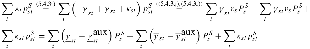
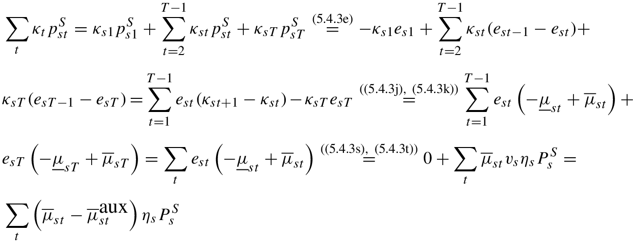
Equations (5.4.3a)–(5.4.3f) ensure primal feasibility. The stationary conditions for each primal variable is ensured through (5.4.3g)–(5.4.3k). Dual feasibility is imposed by constraints (5.4.3l). Finally, constraints (5.4.3m)–(5.4.3t) represent the complementarity conditions. It can be observed that the complementarity conditions include the product of two continuous variables. Therefore, if the lower-level problem (5.4.2f)–(5.4.2l) is replaced by (5.4.3), the rendered optimization problem would be highly nonconvex and global optimality would not be guaranteed. This is a common problem in bilevel programming.


5.4.3 Linearization of MPEC


Although all constraints of (5.4.6) are now linear, the objective function includes nonlinear terms  and
and  . In order to solve this problem computationally efficiently, it is desirable to convert the current MINLP (5.4.6) into a MILP. To that purpose, we must linearize the nonlinear terms in the objective function.
 using some of the optimality conditions of the lower-level problem as follows [58]:
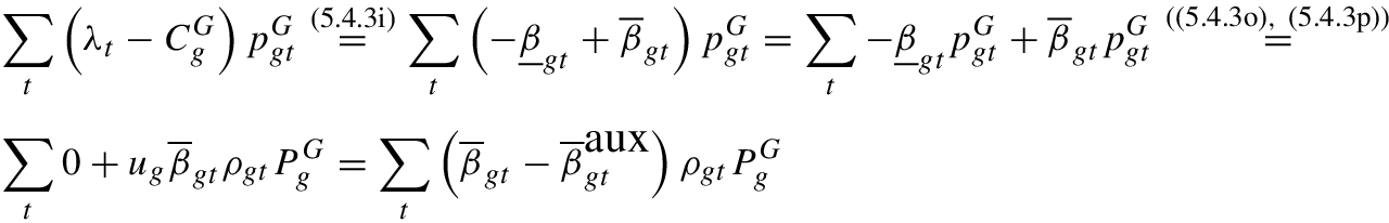


Given valid bounds on some dual variables of the lower-level problem, optimization problem (5.4.10) is an equivalent single-level mixed-integer reformulation of the original bilevel problem (5.4.2) and can thus be solved using commercial software as CPLEX.1 Importantly, this reformulation does not require additional binary variables, and then its computational complexity is comparable to that of its centralized version formulated in (5.4.1). However, it is important to bring to light that finding such valid bounds on dual variables is proven to be NP-hard even for linear bilevel problems [35]. Although some heuristic methods have been proposed to determine bounds of dual variables in a reasonable time, caution must always be exercised when claiming that the optimal global solution of (5.4.10) is also an optimal global solution of (5.4.2). In other words, if the selection of these bounds artificially limits the dual variables, the equivalence between the original bilevel problem and the single-level reformulation is no longer valid.
5.4.4 Illustrative Case Study
Demand and solar capacity factor profiles for the representative day
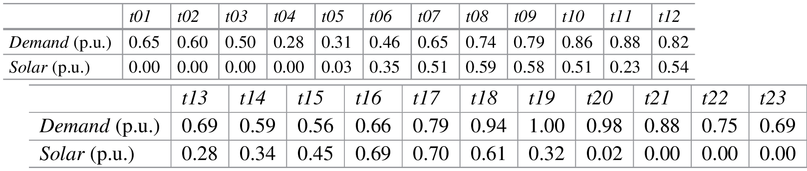
Thermal power generation consisting of combined cycle gas turbine (CCGT) units with a capacity of 100 MW, a linear production cost of 60 €/MWh, and an annualized investment cost of 42,000 €/MW. Failures of thermal units are not considered and therefore ρ gt = 1.
Solar power generating consisting of solar farms with a capacity of 100 MW, a variable production cost equal to 0 €/MWh, and an annualized investment cost of 85,000 €/MW. The capacity factor of these units is provided in Table 5.1.
Energy storage consisting of Lithium-Ion batteries with a power capacity of 100 MW, the discharge time of 4 h, and an annualized investment cost of 4000 €/MW, which is associated with a low-cost projection of this technology in the following years.
- The MI withholds thermal and solar capacity to create scarcity in the system, which causes the total investment costs to be higher in the centralized approach.Table 5.2
Result comparison for strategic and centralized approach
Strategic
Centralized
Thermal capacity (MW)
600
700
Solar capacity (MW)
300
1000
Storage capacity (MW)
400
300
Load shedding (%)
1.8
0
Investment costs (M€)
52
116
Operating costs (M€)
348
218
Total costs (M€)
400
334
Average price (€/MWh)
300
60
Power producer profit (M€)
1431
32
The lack of capacity investment of the MI leads to some demand shedding, which, in turn, increases the operating costs if compared with the centralized approach.
If the investor behaves strategically, the total cost obtained is significantly higher due to the exercise of market power.
In the strategic approach, the electricity price is always equal to C S due to the load shedding actions caused by the limited investments in generation.
The power producer profit is much higher for the strategic approach because of the price increase caused by withholding generating capacity.
A centralized planner would have never captured the fact that a MI strategically withholds capacity to drive up market prices (and even cause load shedding) in order to increase profits.
Bilevel models provide invaluable insight when exploring the strategic behavior of agents in electricity markets.
5.4.5 Alternative Formulation
For the sake of simplicity, we considered discrete investment decisions in this section. This makes sense for large thermal-based generating units that take advantage of the economy of scale. For example, most nuclear power plants have a capacity of 1000 MW approximately. On the contrary, investment in renewable-based power plants such as wind or solar farms allows for a broader range of economically profitable capacities. Hence, one may argue that investment decisions for some projects should be considered as continuous variables. Although this may look like a small variation, it completely changes both the procedure to obtain the equivalent single-level optimization problem and the computational burden of the solution strategy.
 and
and  cannot be linearized as explained in [21]. Therefore, replacing the complementarity conditions by the strong duality condition does not imply any modeling advantage. Alternatively, we can use the method proposed in [22] to reformulate the KKT conditions (5.4.3a)–(5.4.3t) as follows:


Optimization problem (5.4.12) is significantly more complicated than (5.4.10) because: it includes a nonconvex objective function and therefore, globally optimal solutions can hardly ever be guaranteed; the nonconvex term in the objective function could be linearized by discretizing price, for example, however, this yields another problem of loss of feasible (and potentially optimal) solutions; it requires a large number of additional binary variables  ; it requires additional valid bounds on dual variables
  ; it requires additional large enough constants M
1, M
2, M
3, M
4, M
5, M
6, M
7, M
8.
; it requires additional large enough constants M
1, M
2, M
3, M
4, M
5, M
6, M
7, M
8.
Hence, investigating methods to efficiently solve single-level reformulations of bilevel problems such as (5.4.12) is one of the current challenges discussed in Sect. 5.3.
5.5 Conclusions
This chapter provides a general overview of the many applications of bilevel optimization in energy and electricity markets, ranging from transmission and generation expansion planning, to strategic scheduling and bidding, to numerous applications involving energy storage, to natural gas markets, to TSO-DSO interactions or even to electric vehicle aggregators. After a brief discussion on available solution methods for bilevel programs, we point out the specific challenges of bilevel optimization in energy, topics such as: handling the nonconvexity of the full AC OPF formulation; incorporating storage technologies and inter-temporal constraints, which are closely linked to the representation of time in and the computational complexity of power system models; incorporating UC constraints involving binary variables in lower levels of bilevel problems; developing computational methods to solve bilevel problems more efficiently; and, extending them to include stochasticity.
In order to demonstrate the important insights that can be gained from bilevel problems, we present an application of a strategic agent that can invest in thermal, renewable and storage units while considering the feedback from a perfectly competitive market. We formulate the arising MPEC of such a merchant investor and show how to linearize it efficiently. In an illustrative example we compare the strategic investment decisions to the ones of a centralized planner and identify that a strategic agent has incentives to withhold capacity in order to raise market prices. Such behavior could not have been captured by a centralized planning model. This simple example perfectly illustrates that bilevel models are extremely useful to capture trends and decisions made by strategic agents in energy and electricity markets.
This work has been supported by Project Grants ENE2016-79517-R and ENE2017-83775-P, awarded by the Spanish Ministerio de Economia y Competitividad.