© Springer Nature Switzerland AG 2020

S. Dempe, A. Zemkoho (eds.)Bilevel OptimizationSpringer Optimization and Its Applications161https://doi.org/10.1007/978-3-030-52119-6_7

7. Bilevel Optimization and Variational Analysis

Boris S. Mordukhovich¹  

(1)

Department of Mathematics, Wayne State University, Detroit, MI, USA

 

 

Boris S. Mordukhovich

Email: boris@math.wayne.edu

Abstract

This chapter presents a self-contained approach of variational analysis and generalized differentiation to deriving necessary optimality conditions in bilevel optimization with Lipschitzian data. We mainly concentrate on optimistic models, although the developed machinery also applies to pessimistic versions. Some open problems are posed and discussed.

Keywords

Bilevel optimizationVariational analysisNondifferentiable programmingGeneralized differentiationLipschitzian functions and mappings

7.1 Introduction

Bilevel optimization has been well recognized as a theoretically very challenging and practically important area of applied mathematics. We refer the reader to the monographs [2, 6, 14, 30, 41], the extensive bibliographies and commentaries therein, as well as to the advanced material included in this book for various approaches, theoretical and numerical results, and a variety of practical applications of bilevel optimization and related topics.

One of the characteristic features of bilevel optimization problems is their intrinsic nonsmoothness, even if their initial data are described by linear functions. This makes natural to develop an approach of modern variational analysis and generalized differentiation to the study and applications of major models in bilevel optimization. It has been done in numerous publications, which are presented and analyzed in the author’s recent book [30].

The main goal we pursue here is to overview this approach together with the corresponding machinery of variational analysis and to apply it to deriving necessary optimality conditions in optimistic bilevel models with Lipschitzian data while also commenting on other versions in bilevel optimization with posting open questions. To make this chapter largely self-contained and more accessible for the reader, we present here the basic background from variational analysis and generalized differentiation, which is needed for applications to bilevel optimization. For brevity and simplicity we confine ourselves to problems in finite-dimensional spaces.

The rest of this work is organized as follows. In Sect. 7.2 we recall those constructions of generalized differentiation in variational analysis, which are broadly used in the subsequent text. Section 7.3 presents the fundamental extremal principle that is behind generalized differential calculus and applications to optimization in the geometric approach to variational analysis developed in [29, 30]. Section 7.4 is devoted to deriving—via the extremal principle—the two basic calculus rules, which are particularly useful for applications to optimality conditions. In Sect. 7.5 we establish subdifferential evaluations and efficient conditions that ensure the local Lipschitz continuity of optimal value functions in general problems of parametric optimization. These results are crucial for variational applications to bilevel programming.

To proceed with such applications, we first consider in Sect. 7.6 problems of nondifferentiable programming with Lipschitzian data. Subdifferential necessary optimality conditions for Lipschitzian programs are derived there by using the extremal principle and calculus rules. Section 7.7 contains the formulation of the bilevel optimization problems under consideration and the description of the variational approach to their study. Based on this approach and subdifferentiation of the optimal value functions for lower-level problems, we establish in Sect. 7.8 necessary optimality conditions for Lipschitzian bilevel programs. The other developments in this direction for bilevel optimization problems with Lipschitzian data is presented in Sect. 7.9 by using the subdifferential difference rule based on a certain variational technique. The concluding Sect. 7.10 discusses further perspectives of employing concepts and techniques of variational analysis to bilevel optimization with formulations of some open questions.

Throughout this chapter we use the standard notation and terminology of variational analysis and generalized differentiation; see, e.g., [29, 30, 40].

7.2 Basic Constructions of Generalized Differentiation

Here we present the basic definitions of generalized normals to sets, coderivatives of set-valued mappings, and subgradients of extended-real-valued functions initiated by the author [26] that are predominantly used in what follows. The reader is referred to the books [29, 30, 40] for more details. Developing a geometric approach to generalized differentiation, we start with normals to sets, then continue with coderivatives of (set-valued and single-valued) mappings, and finally pass to subgradients of extended-real-valued functions.

Given a nonempty set , we always suppose without loss of generality that it is locally closed around the reference point . For each close to consider its (nonempty) Euclidean projector to Ω defined by

Then the (basic, limiting, Mordukhovich) normal cone to Ω at is

(7.2.1)

The normal cone (7.2.1) is always closed while may be nonconvex in standard situations; e.g., when Ω is the graph of the simplest nonsmooth convex function |x| at . Nevertheless, this normal cone and the associated coderivatives of mappings and subdifferentials of functions enjoy comprehensive calculus rules due to variational/extremal principles of variational analysis. Note that if and only if is a boundary point of Ω.

There is a useful representation of the normal cone (7.2.1) in terms of convex collections of (pre)normal vectors to Ω at points nearby . Given x ∈ Ω close to , the prenormal cone to Ω at x (known also as the regular or Fréchet normal cone) is defined by

(7.2.2)

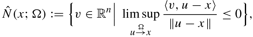
where the symbol means that u → x with u ∈ Ω. Then the prenormal cone (7.2.2) is always closed and convex while may collapse to {0} at boundary points of closed sets, which in fact contradicts the very meaning of generalized normals. If Ω is convex, then both normal and prenormal cones reduce to the normal cone of convex analysis. In general we have

(7.2.3)

bNote that the limiting representation (7.2.3) keeps holding if the prenormal cone (7.2.2) therein is expanded to its ε _k-enlargements as ε _k ↓ 0, where the latter expansions are defined by replacing 0 with ε _k on the right-hand side of (7.2.2).

Let be a set-valued mapping/multifunction with values and with its domain and graph defined, respectively, by

When F is single-valued, we use the standard notation . Assuming that the graph of F is locally closed around , we define the coderivative of F at this point via the normal cone (7.2.1) to the graph of F by

(7.2.4)

Thus is a set-valued positively homogeneous mapping, which reduces to the adjoint/transposed Jacobian for all single-valued mappings that are smooth around , where is dropped in this case in the coderivative notation:

Besides a full calculus available for the coderivative (7.2.4), this construction plays an important role in variational analysis and its applications since it provides complete characterizations of fundamental well-posedness properties of multifunctions concerning Lipschitzian stability, metric regularity, and linear openness/covering. In this work we deal with the Lipschitz-like (Aubin, pseudo-Lipschitz) property of around defined as follows: there exist neighborhoods U of and V  of and a constant ℓ ≥ 0 such that

(7.2.5)

where stands for the closed unit ball of the space in question. If in (7.2.5), then it reduces to the classical local Lipschitzian property of F around . The coderivative characterization of (7.2.5), which is called in [40] the Mordukhovich criterion, tells us that F is Lipschitz-like around if and only if we have

(7.2.6)

Furthermore, the exact bound (infimum) of all the Lipschitz constant {ℓ} in (7.2.5) is calculated as the norm of the positively homogeneous coderivative mapping . The reader can find in [28–30, 40] different proofs of this result with numerous applications.

Consider finally an extended-real-valued function finite at and lower semicontinuous (l.s.c.) around this point. Denote by

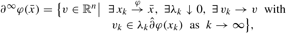
the domain and epigraph of φ, respectively. Given and using the normal cone (7.2.1) to the epigraph of φ at , we define the two types of the subdifferentials of φ at : the basic subdifferential and the singular subdifferential by, respectively,

(7.2.7)

(7.2.8)

The basic subdifferential (7.2.7) reduces to the gradient for smooth functions and to the subdifferential of convex analysis if φ is convex. Observe that and via the coderivative (7.2.4) of the epigraphical multifunction defined by . Thus the coderivative characterization (7.2.6) of the Lipschitz-like property of multifunctions implies that a lower semicontinuous function φ is locally Lipschitzian around if and only if

(7.2.9)

Note also that, given any (closed) set with its indicator functionδ(x; Ω) = δ _Ω(x) equal 0 for x ∈ Ω and ∞ otherwise, we have that

(7.2.10)

Both subdifferentials (7.2.7) and (7.2.8) admit limiting representations in terms of the presubdifferential, or regular subdifferential

(7.2.11)

of φ at points x close to . Namely, we have

(7.2.12)

(7.2.13)

where the symbol indicates that with . Note that the presubdifferential (7.2.11) is related to the prenormal cone (7.2.2) as in (7.2.7) and is also used in variational analysis under the names of the Fréchet subdifferential and the viscosity subdifferential. Similarly to the case of basic normals in (7.2.3) it is not hard to observe that we still have the subdifferential representations in (7.2.12) and (7.2.13) if the presubdifferential (7.2.11) therein is expanded by its ε _k-enlargements defined with replacing 0 on the right-hand side of (7.2.11) by − ε _k.

7.3 Extremal Principle in Variational Analysis

In this section we recall, following [22], the notion of locally extremal points for systems of finitely many sets and then derive the fundamental extremal principle, which gives us necessary conditions for extremality of closed set systems in .

Definition 7.3.1

Let Ω₁, …, Ω_s as s ≥ 2 be nonempty subsets of , which are assumed to be locally closed around their common point . We say that is a Locally Extremal Point of the set system { Ω₁, …, Ω_s} if there exist a neighborhood U of and sequences of vectors , such that a _ik → 0 as k →∞ for all i ∈{1, …, s} and

(7.3.1)

△

Geometrically Definition 7.3.1 says that is a locally extremal point of the set system { Ω₁, …, Ω_s} if these sets can be pushed apart from each other locally around . Observe also that for the case of two sets Ω₁, Ω₂ containing the above definition can be equivalently reformulated as follows: there is a neighborhood U of such that for any ε > 0 there exists a vector with ∥a∥≤ ε and ( Ω₁ − a) ∩ Ω₂ ∩ U = ∅.

It is easy to see that for a closed set Ω and any of its boundary points , we have that is a locally extremal point of the set system . Furthermore, the introduced notion of set extremality covers various notions of optimality and equilibria in problems of scalar and vector optimization. In particular, a local minimizer of the general constrained optimization problem

where φ is l.s.c. and Ω is closed around , corresponds to the locally extremal point of the sets Ω₁ := epi φ and . As we see below, extremal systems naturally arise in deriving calculus rules of generalized differentiation.

Now we are ready to formulate and prove the basic extremal principle of variational analysis for systems of finitely many closed sets in by using the normal cone construction (7.2.1).

Theorem 7.3.2

Let be a locally extremal point of the system { Ω ₁, …, Ω _s} of nonempty subsets of , which are locally closed around . Then there exist generalized normals for i = 1, …, s, not equal to zero simultaneously, such that we have the generalized Euler equation

(7.3.2)

△

Proof

Using Definition 7.3.1, suppose without loss of generality that . Taking the sequences {a _ik} therein, for each k = 1, 2, … consider the unconstrained optimization problem:

(7.3.3)

where d(x; Ω) indicates the Euclidean distance between x and Ω. Since φ _k is continuous and the level sets of it are bounded, we deduce from the classical Weierstrass theorem that there exists an optimal solution x _k to each problem (7.3.3) as k = 1, 2, …. It follows from the crucial extremality requirement (7.3.1) in Definition 7.3.1 that

(7.3.4)

The optimality of x _k in (7.3.3) tells us that

and so γ _k ↓ 0 and as k →∞. By the closedness of the sets Ω_i, i = 1, …, s, around , we pick w _ik ∈ Π(x _k + a _ik; Ω_i) and for each k form another unconstrained optimization problem:

(7.3.5)

which obviously has the same optimal solution x _k. In contrast to φ _k in (7.3.3), the function ψ _k in (7.3.5) is differentiable at x _k due to (7.3.4). Thus applying the Fermat rule in (7.3.5) tells us that

(7.3.6)

with v _ik := (x _k + a _ik − w _ik)∕γ _k, i = 1, …, s, satisfying

(7.3.7)

Remembering the compactness of the unit sphere in , we get by passing to the limit as k →∞ in (7.3.6) and (7.3.7) that there exist v ₁, …, v _s, not equal to zero simultaneously, for which (7.3.2) holds. Finally, it follows directly from the above constructions and the normal cone definition (7.2.1) that for all i = 1, …, s. This completes the proof of the theorem. □

Since for convex sets Ω the normal cone (7.2.1) reduces to the normal cone of convex analysis

the extremal principle of Theorem 7.3.2 can be treated as a variational extension of the classical separation theorem to the case of finitely many nonconvex sets in .

7.4 Fundamental Calculus Rules

Employing the extremal principle, we derive here two fundamental rules of generalized differential calculus, which are broadly used in this chapter and from which many other calculus rules follow; see [29, 30]. The first result is the intersection rule for basic normals (7.2.1).

Theorem 7.4.1

Let Ω ₁, …, Ω _sbe nonempty subsets of , which are locally closed around their common point . Assume the validity of the following qualification condition:

(7.4.1)

Then we have the normal cone intersection rule

(7.4.2)

△

Proof

Arguing by induction, we first verify the result for s = 2. Pick any and use the normal cone representation (7.2.3). It gives us sequences with x _k ∈ Ω₁ ∩ Ω₂ and v _k → v with as k →∞. Take any sequence ε _k ↓ 0 and construct the sets

These sets are obviously closed around (x _k, 0) ∈ Θ₁ ∩ Θ_2k for all k sufficiently large. Furthermore, it follows from the prenormal cone definition (7.2.2) that there exists a neighborhood U of x _k with

for small numbers γ > 0. Thus the pair (x _k, 0) is a locally extremal point of the set system { Θ₁, Θ_2k} for such k. Applying to this system the extremal principle from Theorem 7.3.2 gives us pairs (u _k, λ _k) from the unit sphere in for which

(7.4.3)

Considering a subsequence of the unit vectors (u _k, λ _k) if needed, we get (u _k, λ _k) → (u, λ) as k →∞ for some with ∥(u, λ)∥ = 1. Passing to the limit in the first inclusion of (7.4.3) gives us , which immediately implies—by the easily verifiable product rule equality for normals to Cartesian products (see, e.g., [29, Proposition 1.2])—that and λ ≤ 0. On the other hand, the limiting procedure in the second inclusion of (7.4.3) leads us by the structure of Θ_2k to

(7.4.4)

To verify (7.4.4), for each rewrite the set Θ_2k as

Using representation (7.2.3) of basic normals via limits of regular ones, for each fixed we find sequences x _km → x _k, α _km ↓ 0, u _km → u _k and λ _km → λ _k as m →∞ such that

whenever The latter means by definition (7.2.2) of regular normals that

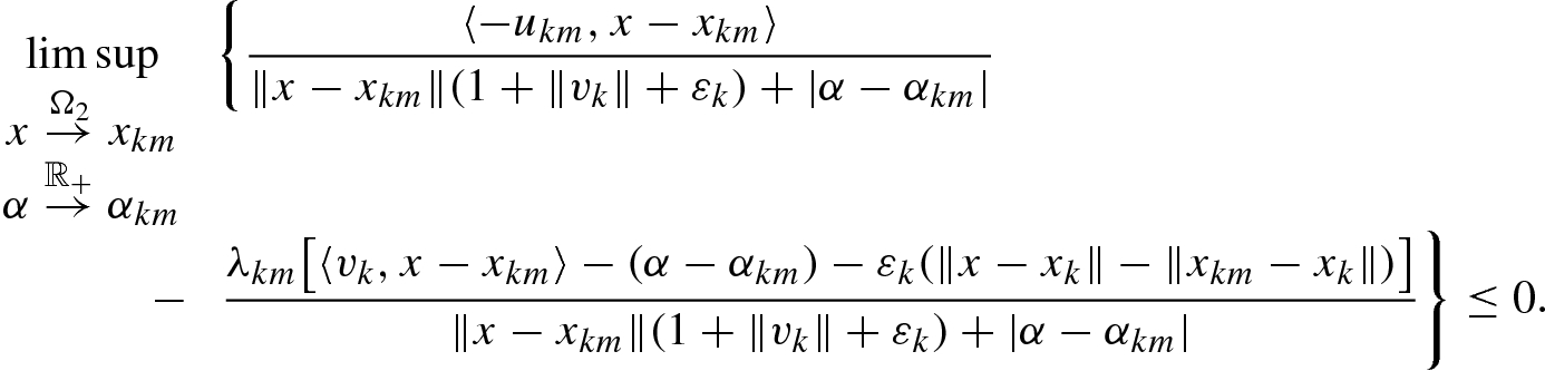
Thus for all and we arrive at the limiting condition

which can be rewritten in terms of ε-enlargements of the prenormal cone as follows:

Employing the standard diagonal process and remembering the representation of basic normals via limits of ε-enlargements of regular ones bring us to the claimed inclusion (7.4.4).

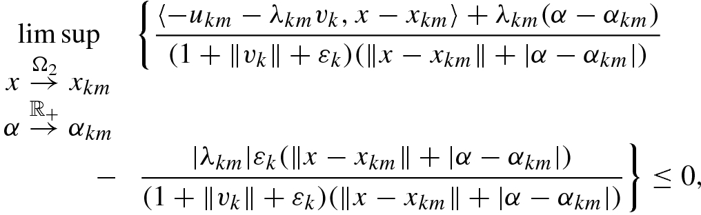
Observe that having λ = 0 in (7.4.4) contradicts the qualification condition (7.4.1) for s = 2. Thus λ < 0, which readily implies that .

To proceed finally by induction for s > 2, we observe that the induction assumption for (7.4.2) in the previous step yields the validity of the qualification condition (7.4.1) needed for the current step of induction. This completes the proof of the theorem. □

Next we derive the subdifferential sum rules concerning both basic subdifferential (7.2.7) and singular subdifferential (7.2.8). For our subsequent applications to bilevel optimization, it is sufficient to consider the case where all but one of the functions involved in summation are locally Lipschitzian around the reference point. This case allows us to obtain the subdifferential sum rules without any qualification conditions.

Theorem 7.4.2

Let be l.s.c. around , and let for i = 2, …, s and s ≥ 2 be locally Lipschitzian around . Then we have the sum rules

(7.4.5)

(7.4.6)

△

Proof

We consider the case where only two functions are under summation since the general case of finitely many functions obviously follows by induction. Let us start with the basic subdifferential sum rule (7.4.5) for s = 2 therein.

Pick any and get by definition (7.2.7) that

Then construct the sets

Denoting , we obviously have that the sets Ω₁ and Ω₂ are locally closed around the triple . It is easy to check that . Applying now to this set intersection the normal cone intersection rule from Theorem 7.4.1, we observe that the qualification condition (7.4.1) is automatically satisfied in this case due to the singular subdifferential characterization (7.2.9) of the local Lipschitz continuity. Hence we get pairs for i = 1, 2 satisfying the condition

which implies that v = v ₁ + v ₂ and λ ₁ = λ ₂ = −1. Therefore it shows that for i = 1, 2, and thus the sum rule (7.4.5) is verified.

Next we proceed with the proof of (7.4.6) for s = 2 starting with verifying the inclusion “⊂” therein. Pick and find by definition sequences , and η _k ↓ 0 such that

whenever (x, μ) ∈epi (φ ₁ + φ ₂) with and |μ − μ _k|≤ η _k as k = 1, 2, …. Taking a Lipschitz constant ℓ > 0 of φ ₂ around , denote and . Then and

for all , and . Therefore

if (x, μ) ∈epi φ ₁ with and . It yields for all k = 1, 2, …, and so since ε _k ↓ 0 as k →∞. This verifies the inclusion “⊂” in (7.4.6). Applying it to the sum φ ₁ = (φ ₁ + φ ₂) + (−φ ₂) yields , which justifies the equality in (7.4.6) and thus completes the proof. □

7.5 Subdifferentials and Lipschitz Continuity of Value Functions

In this section we consider the class of extended-real-valued functions defined by

(7.5.1)

where is an l.s.c. function, and where is a set-valued mapping of closed graph. We can view (7.5.1) as the optimal value function in the problem of parametric optimization described as follows:

with the cost function φ and the constraint mapping F, where y and x are the decision and parameter variables, respectively. Functions of this type are also known in variational analysis under the name of “marginal functions.” A characteristic feature of such functions is their nonsmoothness regardless of the smoothness of the cost function φ and the simplicity of the constraint mapping F that may nicely behave on the parameter x.

As seen below, functions of type (7.5.1) play a crucial role in applications to bilevel optimization while revealing intrinsic nonsmoothness of the latter class of optimization problems. This section presents evaluations of both basic and singular subdifferentials of (7.5.1), which are equally important for the aforementioned applications. Singular subdifferential evaluations are used for establishing the Lipschitz continuity of 𝜗(x) with respect to the parameter x that allows us to reduce the bilevel model under consideration to a single-level problem of Lipschitzian programming. On the other hand, basic subdifferential evaluations open the gate to derive in this way necessary optimality conditions for Lipschitzian bilevel programs.

To proceed, let us consider the argminimum mapping associated with (7.5.1) by

(7.5.2)

and recall that this mapping is inner semicontinuous at if for every sequence there exists a sequence y _k ∈ M(x _k) that converges to as k →∞. Observe that the inner semicontinuity of M at is implied by its Lipschitz-like property at this point.

The following theorem gives us efficient upper estimates of both basic and singular subdifferentials of the optimal value function 𝜗 needed for subsequent applications. We confine ourselves to the case of local Lipschitz continuity of the cost function φ in (7.5.1) that is sufficient to derive necessary optimality conditions for bilevel programs in Sects. 7.8 and 7.9.

Theorem 7.5.1

Let the argminimum mapping (7.5.2) be inner semicontinuous at the point , and let the cost function φ be locally Lipschitzian around this point. Then we have

(7.5.3)

(7.5.4)

△

Proof

To start with the verification of (7.5.3), consider the extended-real-valued function defined via the indicator function of the set gph F by

(7.5.5)

and prove first the fulfillment of the estimate

(7.5.6)

Indeed, pick any subgradient and get from its representation in (7.2.12) sequences and v _k → v with as k →∞. Based on definition (7.2.11), for any sequence ε _k ↓ 0 there exists η _k ↓ 0 as k →∞ such that

This ensures by using the constructions above that

for all y _k ∈ M(x _k) and . This tells us that for all k = 1, 2, …. Employing further the inner semicontinuity of the argminimum mapping M at , we find a sequence of y _k ∈ M(x _k) converging to as k →∞. It follows from imposed convergence that . Hence we arrive at by passing to the limit as k →∞, which verifies therefore the validity of the upper estimate (7.5.6). To derive from (7.5.6) the one in (7.5.3) claimed in the theorem, it remains to use in (7.5.6) the basic subdifferential sum rule (7.4.5) from Theorem 7.4.2 combining it with subdifferentiation of the indicator function in (7.2.10) and the coderivative definition in (7.2.4).

Next we verify the singular subdifferential estimate

(7.5.7)

for optimal value function (7.5.1) in terms of the auxiliary function (7.5.5) under the assumptions made. Picking and taking any sequence ε _k ↓ 0, find by (7.2.13) sequences , and η _k ↓ 0 as k →∞ satisfying

for all , and |μ − μ _k|≤ η _k. The assumed inner semicontinuity of (7.5.2) ensures the existence of sequences and such that

via the ε _k-enlargements of the prenormal cone to the epigraph of ψ. This gives us (7.5.7) by passing to the limit as k →∞. Applying finally to ∂ ^∞ψ in (7.5.7) the singular subdifferential relation (7.4.6) from Theorem 7.4.2 with taking into account the singular subdifferential calculation in (7.2.10) together with the coderivative definition (7.2.4), we arrive at the claimed upper estimate (7.5.4) and thus complete the proof of the theorem. □

As mentioned above, in our applications to bilevel programming we need to have verifiable conditions that ensure the local Lipschitz continuity of the optimal value function (7.5.1). This is provided by the following corollary, which is a direct consequence of Theorem 7.5.1 and the coderivative criterion (7.2.6) for the Lipschitz-like property.

Corollary 7.5.2

In addition to the assumptions of Theorem 7.5.1, suppose that the constraint mapping F is Lipschitz-like around in (7.5.2). Then the optimal value function (7.5.1) is locally Lipschitzian around . △

Proof

We know from the coderivative criterion (7.2.6) that F is Lipschitz-like around if and only if . Applying it to (7.5.4) tells us that the assumed Lipschitz-like property of the constraint mapping F in (7.5.1) ensures that . Furthermore, it easily follows from the assumptions made that the optimal value function is l.s.c. around . Thus 𝜗 is locally Lipschitzian around by the characterization of this property given in (7.2.9). □

7.6 Problems of Lipschitzian Programming

Before deriving necessary optimality conditions in Lipschitzian problems of bilevel optimization in the subsequent sections, we devote this section to problems of single-level Lipschitzian programming. The results obtained here are based on the extremal principle and subdifferential characterization of local Lipschitzian functions while being instrumental for applications to bilevel programs given in Sect. 7.8.

The mathematical program under consideration here is as follows:

(7.6.1)

where the functions , are locally Lipschitzian around the reference point . The next theorem provides necessary optimality conditions in problem (7.6.1) of Lipschitzian programming that are expressed in terms of the basic subdifferential (7.2.7).

Theorem 7.6.1

Let be a feasible solution to problem (7.6.1) that gives a local minimum to the cost function φ ₀therein. Then there exist multipliers λ ₀, …, λ _msatisfying the sign conditions

(7.6.2)

the nontriviality conditions

(7.6.3)

the complementary slackness conditions

(7.6.4)

and the subdifferential Lagrangian inclusion

(7.6.5)

Assume in addition that

(7.6.6)

whenever with . Then the necessary optimality conditions formulated above hold with λ ₀ = 1. △

Proof

Supposing without loss of generality that , consider the point and form the following system of m + 2 sets in the space :

(7.6.7a)

(7.6.7b)

It is obvious that and that all the sets Ω_i, i = 0, …, m + 1, are locally closed around . Furthermore, there exists a neighborhood U of the local minimizer such that for any ε > 0 we find ν ∈ (0, ε) ensuring that

(7.6.8)

where with standing at the first position after . Indeed, the negation of (7.6.8) contradicts the local minimality of in (7.6.1). Having (7.6.8) gives us (7.3.1) for the set system in (7.6.7a), (7.6.7b) and thus verifies that is a locally extremal point of these sets. Applying now the extremal principle from Theorem 7.3.2 to { Ω₀, …, Ω_m+1} at with taking into account the structures of Ω_i, we get , and satisfying the inclusions

(7.6.9)

together with the relationships

(7.6.10)

(7.6.11)

It easily follows from (7.6.9) and the structure of the epigraphical sets in (7.6.9) that the sign conditions (7.6.2) are satisfied. If we suppose while arguing by contradiction to (7.6.3) that λ ₀ = … = λ _m = 0, then ξ = 0 by (7.6.11). Furthermore, the singular subdifferential criterion (7.2.9) for the local Lipschitz continuity of the functions φ _i as i = 0, …, m being combined with the sign conditions (7.6.2) and the definitions (7.2.7) and (7.2.8) of the basic and singular subdifferentials, respectively, tells us that the inclusions in (7.6.9) are equivalent to

(7.6.12)

and hence we get v ₀ = … = v _m = 0. This clearly violates (7.6.10) and thus verifies (7.6.3). The generalized Euler equation in (7.6.11) clearly reduces to the Lagrangian inclusion (7.6.5).

To check further the complementary slackness conditions in (7.6.4), fix i ∈{1, …, m} and suppose that . Then the continuity of φ _i at ensures that the pair is an interior point of the epigraphical set epi φ _i. It readily implies that , and hence λ _i = 0. This yields , which justifies (7.6.4).

To complete the proof of the theorem, it remains to check that the validity of (7.6.6) ensures that λ ₀ = 1 in (7.6.5). We easily arrive at this assertion while arguing by contradiction. □

If the constraint functions φ _i, i = 1, …, m, are smooth around the reference point , condition (7.6.6) clearly reduces to the classical Mangasarian-Fromovitz constraint qualification. It suggests us to label this condition (7.6.6) as the generalized Mangasarian-Fromovitz constraint qualification, or the generalized MFCQ.

7.7 Variational Approach to Bilevel Optimization

This section is devoted to describing some models of bilevel programming and a variational approach to them that involves nondifferentiable optimal value functions in single-level problems of parametric optimization.

Let us first consider the following problem of parametric optimization with respect to the decision variable under each fixed parameter :

(7.7.1)

where is the cost function and is the constraint mapping in (7.7.1), which is called the lower-level problem of parametric optimization. Denoting by

(7.7.2)

the parameterized solution set for (7.7.1) for each and given yet another cost function , we consider the upper-level parametric optimization problem of minimizing ψ(x, y) over the lower-level solution map from (7.7.2) written as:

(7.7.3)

The optimistic bilevel programming model is defined by

(7.7.4)

and where be a given constraint set. On the other hand, the pessimistic bilevel programming model is defined as follows:

(7.7.5)

We refer the reader to [5–8, 11–16, 19, 30, 45, 47, 48], and the bibliographies therein for more details on both optimistic and pessimistic versions in bilevel programming, their local and global solutions as well as reformulations, modifications and relationships with other classes of optimization problems, theoretical and numerical developments, and various applications in finite-dimensional spaces. Investigations and applications of bilevel optimization problems in infinite dimensions can be found, e.g., in [1, 3, 8, 15, 17, 18, 20, 21, 23, 24, 34, 36, 37, 42, 43].

The main attention in this and subsequent sections is paid to the application of the machinery and results of variational analysis and generalized differentiation to problems of bilevel optimization by implementing the value function approach. This approach is based on reducing bilevel programs to single-level problems of mathematical programming by using the nonsmooth optimal value function𝜗(x) of the lower-level problem defined in (7.5.1). Such a device was initiated by Outrata [35] for a particular class of bilevel optimization problems and was used by him for developing a numerical algorithm to solve bilevel programs. Then this approach was strongly developed by Ye and Zhu [44] who employed it to derive necessary optimality conditions for optimistic bilevel programs by using Clarke’s generalized gradients of optimal value functions. More advanced necessary optimality conditions for optimistic bilevel programs in terms of the author’s generalized differentiation reviewed in Sect. 7.2 were developed in [11, 12, 30, 34, 46, 47]. Optimality and stability conditions for pessimistic bilevel models were derived in [13, 16].

We restrict ourselves in what follows to implementing variational analysis and the aforementioned machinery of generalized differentiation within the value function approach to optimistic bilevel models with Lipschitzian data in finite-dimensional spaces. This allows us to most clearly communicate the basic variational ideas behind this approach, without additional technical complications. The variational results presented in the previous sections make our presentation self-contained and complete.

For simplicity we consider the optimistic bilevel model (7.7.4) with only inequality constraints on the lower and upper levels described by

(7.7.6)

(7.7.7)

The reduction of the bilevel program (7.7.4) with the constraints (7.7.6) and (7.7.7) to a single-level problem of nondifferentiable programming and deriving in this way necessary optimality conditions for it are given in the next section.

7.8 Optimality Conditions for Lipschitzian Bilevel Programs

The optimal value function (7.5.1) for the lower-level program (7.7.1) with the inequality constraints specified in (7.7.6) reads as

(7.8.1)

With the upper-level cost function ψ given in (7.7.3) and the upper-level constraints taken from (7.7.7), consider the following single-level mathematical program with inequality constraints:

(7.8.2)

We can easily observe that global optimal solutions to (7.8.2) agree with those to problem (7.7.4), (7.7.6), and (7.7.7). Although this is not always the case for local minimizers, it holds under the inner semicontinuity assumption on the solution map associated with the optimistic bilevel program (7.7.4); see [12, Proposition 6.9] for the precise statement.

Looking at (7.8.2), observe that this problem is of type (7.6.1) for which necessary optimality conditions are given in Theorem 7.6.1, provided that all the functions involved are locally Lipschitzian. However, the direct application of Theorem 7.6.1 to problem (7.8.2) is not efficient due to the structure of the last constraint therein defined via the lower-level optimal value function (7.8.1). Indeed, it has been realized in bilevel programming that this constraint prevents the fulfillment of conventional constraint qualifications; in particular, the generalized MFCQ (7.6.6). To avoid this obstacle, Ye and Zhu [44] introduced the following property postulating an appropriate behavior of the cost function in (7.8.2) with respect to linear perturbations of the constraint φ(x, y) ≤ 𝜗(x). Consider the problem:

(7.8.3)

Definition 7.8.1

Problem (7.8.2) is Partially Calm at its local optimal solution if there exist a constant κ > 0 and a neighborhood U of such that

(7.8.4)

for all the triples (x, y, ν) ∈ U feasible to (7.8.3). △

There are various efficient conditions, which ensure the fulfillment of the partial calmness property for (7.8.2). They include the uniform sharp minimum condition [44], linearity of the lower-level problem with respect to the decision variable [9], the kernel condition [30], etc. On the other hand, partial calmness may fail in rather common situations; see [19, 30] for more results and discussions on partial calmness and related properties.

The main impact of partial calmness to deriving necessary optimality conditions for (7.8.2) is its equivalence to the possibility of transferring the troublesome constraint φ(x, y) ≤ 𝜗(x) into the penalized cost function as in the following proposition.

Proposition 7.8.2

Let problem (7.8.2) be partially calm at its local optimal solution with ψ being continuous at this point. Then is a local optimal solution to the penalized problem

(7.8.5)

where the number κ > 0 is taken from (7.8.4). △

Proof

Taking κ and U from Definition 7.8.1 and using the continuity of ψ at , we find γ > 0 and η > 0 with and

Let us employ it to verify that

(7.8.6)

and with F taken from (7.7.6). If , then (7.8.6) follows from (7.8.4). In the remaining case where , we get that

which also yields (7.8.6) by . The feasibility of to (7.8.2) tells us that , which thus verifies the claimed statement. □

Thus the imposed partial calmness allows us to deduce the original problem of optimistic bilevel optimization to the single-level mathematical program (7.8.5) with conventional inequality constraints, where the troublesome term φ(x, y) − 𝜗(x) enters the penalized cost function. To derive necessary optimality conditions for (7.8.5), let us reformulate the generalized MFCQ (7.6.6) in conventional bilevel terms as in the case of bilevel programs with smooth data [6].

We say that is lower-level regular if it satisfies the generalized MFCQ in the lower-level problem (7.7.1). This means due to the structure of (7.7.1) that

(7.8.7)

whenever with some and

Similarly, a point satisfying the upper-level constraints in (7.7.7) is upper-level regular if

(7.8.8)

with the active constraint indexes .

Now we are ready for the application of Theorem 7.6.1 to the optimistic bilevel program in the equivalent form (7.8.5). To proceed, we have to verify first that the optimal value function 𝜗(x) in the cost function of (7.8.5) is locally Lipschitzian around the reference point and then to be able to upper estimate the basic subdifferential (7.2.7) of the function − 𝜗(⋅). Since the basic subdifferential does not possess the plus-minus symmetry while its convex hull does, we need to convexify in the proof the set on the right-hand side of the upper estimate in (7.5.3). In this way we arrive at the following major result.

Theorem 7.8.3

Let be a local optimal solution to the optimistic bilevel program in the equivalent form (7.8.2) with the lower-level optimal value function 𝜗(x) defined in (7.8.1). Assume that all the functions φ, ψ, f _i, g _jare locally Lipschitzian around the reference point, that the lower-level solution map S from (7.7.2) is inner semicontinuous at , that the lower-level regularity (7.8.7) and upper-level regularity (7.8.8) conditions hold, and that problem (7.8.2) is partially calm at with constant κ > 0. Then there exist multipliers λ ₁, …, λ _r, μ ₁, …, μ _s, and ν ₁, …, ν _rsatisfying the sign and complementary slackness conditions

(7.8.9)

(7.8.10)

(7.8.11)

together with the following relationships, which involve some vector

(7.8.12)

(7.8.13)

△

Proof

It follows from Proposition 7.8.2 that is a local minimizer of the mathematical program (7.8.5) with inequality constraints. To show that it belongs to problems of Lipschitzian programming considered in Sect. 7.6, we need to check that the optimal value function (7.8.1) is locally Lipschitzian around under the assumptions made. This function is clearly l.s.c. around , and thus its Lipschitz continuity around this point is equivalent to the condition . It follows from the upper estimate (7.5.4) of Theorem 7.5.1 and the assumed inner semicontinuity of the solution map (7.7.2) at that

Corollary 7.5.2 tells us that the local Lipschitz continuity of 𝜗 around follows from the Lipschitz-like property of the mapping . Since

we deduce that from the assumed lower-level regularity due to the coderivative definition and the normal come intersection rule in Theorem 7.4.1. Thus F is Lipschitz-like around by the coderivative criterion (7.2.6), and the Lipschitz continuity of 𝜗(⋅) is verified.

Now we can apply to problem (7.8.5) the necessary optimality conditions for Lipschitzian programs obtained in Theorem 7.6.1. The assumed lower-level regularity and upper-level regularity clearly imply that the generalized MFCQ condition (7.6.6) holds. Thus there are multipliers λ ₁, …, λ _r and μ ₁, ⋯ , μ _s satisfying the sign and complementary slackness conditions in (7.8.9) and (7.8.10) for which we have

(7.8.14)

To estimate in (7.8.14), recall that

where stands for Clarke’s generalized gradient of locally Lipschitzian functions that possesses the plus-minus symmetry property [4]. Using it in (7.8.14), we get such that

(7.8.15)

Applying the convexified subdifferential estimates (7.5.3) from Theorem 7.5.1 to the optimal value function (7.8.1) allows us to find multipliers ν ₁, …, ν _r satisfying the sign and complementary slackness conditions in (7.8.11) that ensure the validity of (7.8.12). To verify finally (7.8.13), we divide (7.8.15) by κ > 0 with keeping the same notation for the scaled multipliers λ _i and μ _j. □

The next section presents an independent set of necessary optimality conditions for optimistic bilevel programs with Lipschitzian data that are obtained without using any convexification while employing instead yet another variational device and subdifferential calculus rule.

7.9 Bilevel Optimization via Subdifferential Difference Rule

Considering the single-level problem (7.8.5), which we are finally dealing with while deriving necessary optimality conditions for optimistic bilevel programs, note that the objective therein contains the difference of two nonsmooth functions. The basic subdifferential (7.2.7) does not possesses any special rule for difference of nonsmooth functions, but the regular subdifferential (7.2.11) does, as was first observed in [33] by using a smooth variational description of regular subgradients. Here we employ this approach to establish necessary optimality conditions for Lipschitzian bilevel programs that are different from those in Theorem 7.8.3.

The derivation of these necessary optimality conditions is based on the following two results, which are certainly of their independent interest. The first one provides a smooth variational description of regular subgradients of arbitrary functions .

Lemma 7.9.1

Let be finite at , and let . Then there exists a neighborhood U of and a function such that , that ψ is Fréchet differentiable at with , and that the difference ψ − φ achieves at its local maximum on U. △

Proof

We proceed geometrically due to the relationship

which reduces the claimed assertion to the following: if and only if there exists a neighborhood U of and a function such that ψ is Fréchet differentiable at with while achieving at its local maximum relative to Ω.

To verify the latter, observe that for any satisfying the listed properties we get

It shows that , and thus by definition (7.2.2). Conversely, pick and define the function

It is easy to check that this function enjoys all the properties listed above. □

The second lemma gives us the aforementioned difference rule for regular subgradients.

Lemma 7.9.2

Consider two arbitrary functions that are finite at and assume that . Then we have the inclusions

(7.9.1)

It implies, in particular, that any local minimizer of the difference function φ ₁ − φ ₂satisfies the necessary optimality condition

(7.9.2)

△

Proof

Starting with (7.9.1), pick . Then the smooth variational description of v from Lemma 7.9.1 gives us on a neighborhood U of that is differentiable at with

Fix further an arbitrary vector and for any ε > 0 find γ > 0 such that

if . Due to the differentiability of ψ at we use the elementary sum rule for the regular subgradients (see, e.g., [29, Proposition 1.107(i)]) and immediately get the relationships

which clearly verify both inclusions in (7.9.1). Picking further any , we deduce from (7.9.1) and the obvious Fermat stationary rule via regular subgradients that

It shows that and thus verifies the fulfillment of (7.9.2). □

Now we are in a position to derive refined necessary optimality conditions for optimistic bilevel programs with Lipschitzian data.

Theorem 7.9.3

Let be a local optimal solution to the optimistic bilevel program in the equivalent form (7.8.2) without upper level constraints. Suppose that all the functions φ, ψ, f _iare locally Lipschitzian around the reference point, that the lower-level solution map S in (7.7.2) is inner semicontinuous at , that the lower-level regularity (7.8.7) condition holds, and that problem (7.8.2) is partially calm at with constant κ > 0. Assume in addition that for the optimal value function (7.8.1). Then there exists a vector together with multipliers λ ₁, …, λ _rand ν ₁, …, ν _rfor i = 1, …, r satisfying the sign and complementary slackness conditions in (7.8.11) and (7.8.9), respectively, such that

(7.9.3)

(7.9.4)

△

Proof

We get from the partial calmness penalization in Proposition 7.8.2 employed together with the infinite penalization of the lower-level constraints that a local minimizer for the unconstrained optimization problem

(7.9.5)

with the mapping defined in (7.7.6). Then applying to (7.9.5) the difference rule (7.9.2) from Proposition 7.9.2 gives us the inclusion

(7.9.6)

At the same time it follows from the proof of Theorem 7.5.1 that

(7.9.7)

Replacing by the larger ∂ on the right-hand sides of (7.9.6) and (7.9.7) and then using the basic subdifferential sum rule from Theorem 7.4.2 yield the inclusions

(7.9.8)

Employing in these inclusions Theorem 7.4.1 under the lower-level regularity of with the usage of the singular subdifferential characterization of Lipschitzian functions in (7.2.9), we get

It allows us to deduce from (7.9.8) the existence of ensuring the validity of (7.9.3) and

Dividing the latter by κ > 0, we arrive at (7.9.4) and thus complete the proof of the theorem. □

Observe that we always have if the optimal value function (7.8.1) is convex, which is surely the case when all the functions φ and f _i therein are convex. If in addition the upper-level data are also convex, more general results were derived in [17] for problems of semi-infinite programming with arbitrary number of inequality constraints in locally convex topological vector spaces by reducing them to problems of DC programming with objectives represented as differences of convex functions. Note further that the necessary optimality conditions obtained in Theorems 7.8.3 and 7.9.3 are independent of each other even in the case of bilevel programs with smooth data. In particular, we refer the reader to [30, Example 6.24] for illustrating this statement and for using the obtained results to solve smooth bilevel programs. Finally, we mention the possibility to replace the inner semicontinuity assumption on the solution map S(x) imposed in both Theorems 7.8.3 and 7.9.3 by the uniform boundedness of this map in finite-dimensions, or by its inner semicompactness counterpart in infinite-dimensional spaces; cf. [11, 16, 30, 34] for similar transitions in various bilevel settings.

7.10 Concluding Remarks and Open Questions

In this self-contained chapter of the book we described a variational approach to bilevel optimization with its implementation to deriving advanced necessary optimality conditions for optimistic bilevel programs in finite-dimensional spaces. The entire machinery of variational analysis and generalized differentiation (including the fundamental extremal principle, major calculus rules, and subdifferentiation of optimal value functions), which is needed for this device, is presented here with the proofs. The given variational approach definitely has strong perspectives for further developments. Let us briefly discuss some open questions in this direction.

• The major difference between the optimistic model (7.7.4) and pessimistic model (7.7.5) in bilevel programming is that the latter invokes the supremum marginal/optimal value function instead of the infimum type in (7.7.4). Subdifferentiation of the supremum marginal functions is more involved in comparison with that of the infimum type. Some results in this vein for problems with Lipschitzian data can be distilled from the recent papers [31, 32, 38], while their implementation in the framework of pessimistic bilevel programs is a challenging issue.

• The given proof of the necessary optimality conditions for bilevel programs in Theorem 7.8.3 requires an upper estimate of , which cannot be directly derived from that for since . To obtain such an estimate, we used the subdifferential convexification and the fact that the convexified/Clarke subdifferential of Lipschitz continuous functions possesses the plus-minus symmetry. However, there is a nonconvex subgradient set that is much smaller than Clarke’s one while having this symmetry. It is the symmetric subdifferential , which enjoys full calculus induced by the basic one. Efficient evaluations of for infimum and supremum marginal functions would lead us to refined optimality conditions for both optimistic and pessimistic models in bilevel optimization.

• The partial calmness property used in both Theorems 7.8.3 and 7.9.3 seems to be rather restrictive when the lower-level problem is nonlinear with respect to the decision variable. It is a challenging research topic to relax this assumption and to investigate more the uniform weak sharp minimum property and its modifications that yield partial calmness.

• One of the possible ways to avoid partial calmness in bilevel programming is as follows. Having the solution map to the lower-level problem, consider the constrained upper-level problem given by

(7.10.1)

where is the cost function on the upper level with the upper-level constraint set , and where the minimization of is understood with respect to the standard order on . Then (7.10.1) is a problem of set-valued optimization for which various necessary optimality conditions of the coderivative and subdifferential types can be found in [30] and the references therein. Evaluating the coderivatives and subdifferentials of the composition ψ(x, S(x)) in terms of the given lower-level and upper-level data of bilevel programs would lead us to necessary optimality conditions in both optimistic and pessimistic models. There are many open questions arising in efficient realizations of this approach for particular classes of problems in bilevel optimization even with smooth initial data. We refer the reader to the paper by Zemkoho [47] for some recent results and implementations in this direction.

Note that a somewhat related approach to bilevel optimization was developed in [1], where a lower-level problem was replaced by the corresponding KKT system described by a certain generalized equation of the Robinson type [39]. Applying to the latter necessary optimality conditions for upper-level problems with such constraints allowed us to establish verifiable results for the original nonsmooth problem of bilevel programming.

• Henrion and Surowiec suggested in [19] a novel approach to derive necessary optimality conditions for optimistic bilevel programs with -smooth data and convex lower-level problems. Their approach used a reduction to mathematical programs with equilibrium constraints (MPECs) and allowed them to significantly relax the partial calmness assumption. Furthermore, in this way they obtained new necessary optimality conditions for the bilevel programs under consideration, which are described via the Hessian matrices of the program data.

  A challenging direction of the future research is to develop the approach and results from [19] to nonconvex bilevel programs with nonsmooth data. It would be natural to replace in this way the classical Hessian in necessary optimality conditions by the generalized one (known as the second-order subdifferential) introduced by the author in [27] and then broadly employed in variational analysis and its applications; see, e.g., [30] and the references therein.

• As it has been long time realized, problems of bilevel optimization are generally ill-posed, which creates serious computational difficulties for their numerical solving; see, e.g., [5, 6, 47] for more details and discussions. Furthermore, various regularization methods and approximation procedures devised in order to avoid ill-posedness have their serious drawbacks and often end up with approximate solutions, which may be far enough from optimal ones. Thus it seems appealing to deal with ill-posed bilevel programs how they are and to develop numerical algorithms based on the obtained necessary optimality conditions. Some results in this vein are presented in [47] with involving necessary optimality conditions of the type discussed here, while much more work is required to be done in this very important direction with practical applications.

Acknowledgements

This research was partly supported by the USA National Science Foundation under grants DMS-1512846 and DMS-1808978, by the USA Air Force Office of Scientific Research under grant 15RT04, and by Australian Research Council Discovery Project DP-190100555.

The author is indebted to an anonymous referee and the editors for their very careful reading of the original presentation and making many useful suggestions and remarks, which resulted in essential improvements of the paper.

References

1. 1.
   T.Q. Bao, P. Gupta, B.S. Mordukhovich, Necessary conditions for multiobjective optimization with equilibrium constraints. J. Optim. Theory Appl. 135, 179–203 (2007)
2. 2.
   J.F. Bard, Practical Bilevel Optimization: Algorithms and Applications (Kluwer, Dordrecht, 1998)
3. 3.
   F. Benita, S. Dempe, P. Mehlitz, Bilevel optimal control problems with pure state constraints and finite-dimensional lower level. SIAM J. Optim. 26, 564–588 (2016)
4. 4.
   F.H. Clarke, Optimization and Nonsmooth Analysis (Wiley-Interscience, New York, 1983)
5. 5.
   B. Colson, P. Marcotte, G. Savard, An overview of bilevel optimization. Ann. Oper. Res. 153, 235–256 (2007)
6. 6.
   S. Dempe, Foundations of Bilevel Programming (Kluwer, Dordrecht, 2002)
7. 7.
   S. Dempe, J. Dutta, Is bilevel programming a special case of mathematical programming with complementarity constraints? Math. Program. 131, 37–48 (2012)
8. 8.
   S. Dempe, P. Mehlitz, Semivectorial bilevel programming versus scalar bilevel programming. Optimization (2019). https://​doi.​org/​10.​1080/​02331934.​2019.​1625900
9. 9.
   S. Dempe, A.B. Zemkoho, The bilevel programming problem: reformulations, constraint qualifications and optimality conditions. Math. Program. 138, 447–473 (2013)
10. 10.
    S. Dempe, A.B. Zemkoho, KKT reformulation and necessary conditions for optimality in nonsmooth bilevel optimization. SIAM J. Optim. 24, 1639–1669 (2014)
11. 11.
    S. Dempe, J. Dutta, B.S. Mordukhovich, New necessary optimality conditions in optimistic bilevel programming. Optimization 56, 577–604 (2007)
12. 12.
    S. Dempe, B.S. Mordukhovich, A.B. Zemkoho, Sensitivity analysis for two-level value functions with applications to bilevel programming. SIAM J. Optim. 22, 1309–1343 (2012)
13. 13.
    S. Dempe, B.S. Mordukhovich, A.B. Zemkoho, Necessary optimality conditions in pessimistic bilevel programming. Optimization 63, 505–533 (2014)
14. 14.
    S. Dempe, V. Kalashnikov, G.A. Pérez-Valdés, N. Kalashnikova, Bilevel Programming Problems (Springer, New York, 2015)
15. 15.
    S. Dempe, F. Harder, P. Mehlitz, G. Wachsmuth, Solving inverse optimal control problems via value functions to global optimality. J. Global Optim. 74, 297–325 (2019)
16. 16.
    S. Dempe, B.S. Mordukhovich, A.B. Zemkoho, Two-level value function approach to optimistic and pessimistic bilevel programs. Optimization 68, 433–455 (2019)
17. 17.
    N. Dinh, B.S. Mordukhovich, T.T.A. Nghia, Subdifferentials of value functions and optimality conditions for some classes of DC and bilevel infinite and semi-infinite programs. Math. Program. 123, 101–138 (2010)
18. 18.
    F. Harder, G. Wachsmuth, Optimality conditions for a class of inverse optimal control problems with partial differential equations. Optimization 68, 615–643 (2019)
19. 19.
    R. Henrion, T. Surowiec, On calmness conditions in convex bilevel programming. Appl. Anal. 90, 951–970 (2011)
20. 20.
    G. Holler, K. Kunisch, R.C. Barnard, A bilevel approach for parameter learning in inverse problems. Inverse Probl. 34, 1–28 (2018)
21. 21.
    K. Knauer, C. Büskens, Hybrid solution methods for bilevel optimal control problems with time dependent coupling, in Recent Advances in Optimization and Its Applications in Engineering, ed. by M. Diehl et al. (Springer, Berlin, 2010), pp. 237–246
22. 22.
    A.Y. Kruger, B.S. Mordukhovich, Extremal points and the Euler equation in nonsmooth optimization. Dokl. Akad. Nauk BSSR 24, 684–687 (1980)
23. 23.
    M.B. Lignola, J. Morgan, Inner regularizations and viscosity solutions for pessimistic bilevel optimization problems. J. Optim. Theory Appl. 173, 183–202 (2017)
24. 24.
    P. Mehlitz, G. Wachsmuth, Weak and strong stationarity in generalized bilevel programming and bilevel optimal control. Optimization 65, 907–935 (2017)
25. 25.
    K. Mombaur, A. Truong, J.-P. Laumond, From human to humanoid locomotion–an inverse optimal control approach. Autom. Robots 28, 369–383 (2010)
26. 26.
    B.S. Mordukhovich, Maximum principle in problems of time optimal control with nonsmooth constraints. J. Appl. Math. Mech. 40, 960–969 (1976)
27. 27.
    B.S. Mordukhovich, Sensitivity analysis in nonsmooth optimization, in Theoretical Aspects of Industrial Design, ed. by D.A. Field, V. Komkov. SIAM Proc. Appl. Math., vol. 58 (Philadelphia, Pennsylvania, 1992), pp. 32–46
28. 28.
    B.S. Mordukhovich, Complete characterization of openness, metric regularity, and Lipschitzian properties of multifunctions. Trans. Am. Math. Soc. 340, 1–35 (1993)
29. 29.
    B.S. Mordukhovich, Variational Analysis and Generalized Differentiation, I: Basic Theory, II: Applications (Springer, Berlin, 2006)
30. 30.
    B.S. Mordukhovich, Variational Analysis and Applications (Springer, Cham, 2018)
31. 31.
    B.S. Mordukhovich, T.T.A. Nghia, Subdifferentials of nonconvex supremum functions and their applications to semi-infinite and infinite programs with Lipschitzian data. SIAM J. Optim. 23, 406–431 (2013)
32. 32.
    B.S. Mordukhovich, T.T.A. Nghia, Nonsmooth cone-constrained optimization with applications to semi-infinite programming. Math. Oper. Res. 39, 301–337 (2014)
33. 33.
    B.S. Mordukhovich, N.M. Nam, N.D. Yen, Fréchet subdifferential calculus and optimality conditions in nondifferentiable programming. Optimization 55, 685–396 (2006)
34. 34.
    B.S. Mordukhovich, N.M. Nam, H.M. Phan, Variational analysis of marginal functions with applications to bilevel programming. J. Optim. Theory Appl. 152, 557–586 (2011)
35. 35.
    J.V. Outrata, On the numerical solution of a class of Stackelberg problems. ZOR–Methods Models Oper. Res. 34, 255–277 (1990)
36. 36.
    K.D. Palagachev, M. Gerdts, Exploitation of the value function in a bilevel optimal control problem, in System Modeling and Optimization, ed. by L. Bociu et al. (Springer, Cham, 2016), pp. 410–419
37. 37.
    K.D. Palagachev, M. Gerdts, Numerical approaches towards bilevel optimal control problems with scheduling tasks, in Math for the Digital Factory, ed. by L. Ghezzio et al. (Springer, Cham, 2017), pp. 205–228
38. 38.
    P. Pérez-Aros, Subdifferential formulae for the supremum of an arbitrary family of functions. SIAM J. Optim. 29, 1714–1743 (2019)
39. 39.
    S.M. Robinson, Generalized equations and their solutions, I: basic theory. Math. Program. Study 10, 128–141 (1979)
40. 40.
    R.T. Rockafellar, R.J-B. Wets, Variational Analysis (Springer, Berlin, 1998)
41. 41.
    K. Shimizu, Y. Ishizuka, J.F. Bard, Nondifferentiable and Two-Level Mathematical Programming (Kluwer, Dordrecht, 1997)
42. 42.
    J.J. Ye, Necessary conditions for bilevel dynamic optimization problems. SIAM J. Control Optim. 33, 1208–1223 (1995)
43. 43.
    J.J. Ye, Optimal strategies for bilevel dynamic problems. SIAM J. Control Optim. 35, 512–531 (1997)
44. 44.
    J.J. Ye, D.L. Zhu, Optimality conditions for bilevel programming problems. Optimization 33, 9–27 (1995)
45. 45.
    J.J. Ye, D.L. Zhu, New necessary optimality conditions for bilevel programs by combining MPEC and the value function approach. SIAM J. Optim. 20, 1885–1905 (2010)
46. 46.
    A.J. Zaslavski, Necessary optimality conditions for bilevel minimization problems. Nonlinear Anal. 75, 1655–1678 (2012)
47. 47.
    A. Zemkoho, Solving ill-posed bilevel programs. Set-Valued Var. Anal. 24, 423–448 (2016)
48. 48.
    R. Zhang, Multistage bilevel programming problems. Optimization 52, 605–616 (2003)