9.1 Introduction
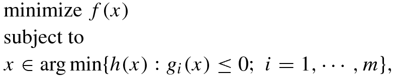
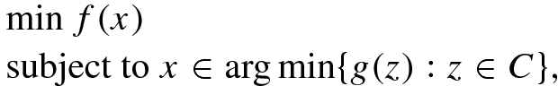
 are convex functions and C a closed convex set in
  . However we could consider
  , where U is an open convex set containing C. Further we can also assume that
  and
and  , where
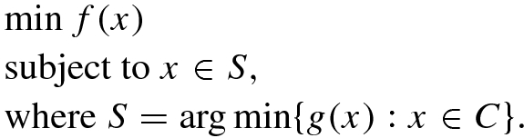
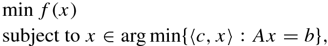
  are proper, lower semi-continuous, convex functions. The problem stated above is called (SBP) to denote the phrase Simple Bilevel Program. The fact that (SBP) has a bilevel structure is evident, while we call it simple since it is represented by only one decision variable in contrast to the two-variable representation in standard bilevel problem. For a detailed discussion on bilevel programming see Dempe [3]. Those readers with an experience in optimization may immediately make the following observation. In general a convex optimization problem may have more than one solution and hence uncountably infinite number of solutions. The decision maker usually would prefer only one among these many solutions. A best way to pick a single solution is to devise a strongly convex objective which is minimized over the solution set of the convex optimization. That gives rise to a simple bilevel problem. The above discussion is explained through the following example.

 is convex, A is an m × n matrix,
  and each
  is convex. Consider the following simple bilevel problem
 and the maximum is taken component-wise i.e.
 , since g(x) ≥ 0 for all
  . This shows that if F is the feasible set of (CP), then
 . This implies that if
  is a solution of (CP), then
  .
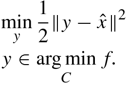
.There is another class of problems where the (SBP) formulation may play role in estimating the distance between a feasible point and the solution set of a convex programming problem. This was discussed in Dempe et al. [7]. However for completeness we will also discuss it here through the following example.

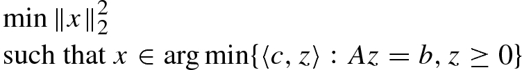
 . For this problem the solution set is given as
 . Given any
  , suppose we want to estimate
  . In general this may not be so easily done. If we consider
  as a system of convex inequalities as shown above in (9.1.1), we can not use the error bound theory in the literature (see for example Lewis and Pang [17] and the references therein) to establish an upper bound to
  , as the Slater’s condition fails for this system of convex inequalities. One way out of this is to use the simple bilevel programming to estimate
  numerically. In fact we can consider the following problem for a given
  ,
, 
 is closed and convex if f and g
i’s are finite-valued and
is closed and convex if f and g
i’s are finite-valued and  is coercive in y and thus a minimizer exists and is unique since
  is strongly convex in y. Let y
∗ be that unique solution, then
is strongly convex in y. Let y
∗ be that unique solution, then 
Note that if in (CP1), f is strongly convex, then an upper bound to 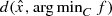 can be computed using the techniques of gap function. See for example Fukushima [24]. If f is convex but not strongly convex then the gap function approach does not seem to work and it appears that at least at present the simple bilevel programming approach is a nice way to estimate
  .
.

 is the i-th component of the vector
  .
.
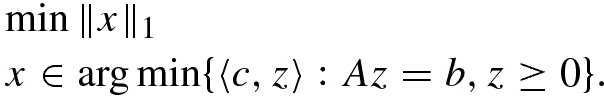
 and F is the feasible set of (LP). Though we can use the Hoffmann error bound to get an upper bound to
  ; that upper bound will depend on
  which is never known before hand. Thus even for the case of (LP) we want to argue that the approach through the simple bilevel formulation is better to estimate
  . Before we end our discussion on this issue we would like to mention that even by using the simple bilevel formulation we are indeed providing an upper bound to
  . Note that while computing the minimizer in the simple bilevel programming formulation, we usually choose an iterate say y
k ∈ C as an approximate solution to the bilevel formulation. Hence
. Note that while computing the minimizer in the simple bilevel programming formulation, we usually choose an iterate say y
k ∈ C as an approximate solution to the bilevel formulation. Hence 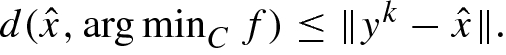
We hope we have been able to convince the reader about the usefulness of the simple bilevel problem. Let us now list down the topics that we shall discuss in rest of the article.
9.2 Optimality and Links with MPCC
 . Then (SBP) can be equivalently reformulated as
 such that
  , then it contradicts the fact that
  . Since Slater’s condition fails one may doubt whether the KKT conditions would hold. One might also feel that KKT conditions might hold under more weaker conditions. The KKT condition for the (SBP), is defined to be the KKT condition for the reformulated problem which we will term as (r-SBP). The KKT conditions at any x feasible to (r-SBP) postulates the existence of λ ≥ 0, such that
 - 1.
0 ∈ ∂f(x) + λ∂g(x) + N C(x)
- 2.
λ(g(x) − α) = 0


 is a m × n matrix and
  . For simplicity let us assume that f is differentiable. Assume that

 such that

 and λ ≥ 0, such that (9.2.2) holds. Then is x
∗ a solution of (SBP)? To answer this question it is important to note that x
∗ is also feasible for (r-SBP) as 〈c, x〉 = α. Now we have the following simple steps which we provide for completeness. For any feasible x for (SBP) we have
and λ ≥ 0, such that (9.2.2) holds. Then is x
∗ a solution of (SBP)? To answer this question it is important to note that x
∗ is also feasible for (r-SBP) as 〈c, x〉 = α. Now we have the following simple steps which we provide for completeness. For any feasible x for (SBP) we have 


 and
and  . Then x
∗ is a solution of the minimum-norm solution problem of the linear programming problem
. Then x
∗ is a solution of the minimum-norm solution problem of the linear programming problem 
 and λ ≥ 0 such that
9.2.1 Simple Bilevel Programming Problem and MPCC
This subsection focuses in the relation between simple bilevel programming problem (9.2.3) and its corresponding MPCC problem. Here we present some results showing that (SBP) problem exactly follows the standard optimistic bilevel programming problem in this context (see [4] for details). We will show that if the lower level problem of the (SBP) satisfies the Slater condition then it is equivalent to it’s corresponding MPCC problem. Lack of Slater condition leads to counter-examples where (SBP) and related MPCC are not connected in solution sense. The results of this subsection were first presented in the thesis of Pandit [18].
 are convex functions and for each i ∈{1, ⋯ , m} the functions
  are also convex functions. The corresponding MPCC is given by
 such that g(x) ≤ 0, let us define
Let
 be a global minimizer of the simple bilevel programming problem (9.2.3) and assume that the lower level problem satisfies the Slater condition. Then for any
 , the point
 is a global minimizer of the corresponding MPCC Problem (9.2.4). △
 is the minimizer of the (SBP) problem (9.2.3), thus it is a solution of the lower level problem. Since the Slater condition holds for the lower level problem in (9.2.3), we conclude that
 , we have
  to be a feasible point of the (MPCC) problem (9.2.4). Consider any (x, λ′) to be feasible point of the (MPCC) problem (9.2.4), then it is simple to observe by noting the convexity of h and g
i’s we conclude that x is feasible for the (SBP) problem (9.2.3). Hence
to be a feasible point of the (MPCC) problem (9.2.4). Consider any (x, λ′) to be feasible point of the (MPCC) problem (9.2.4), then it is simple to observe by noting the convexity of h and g
i’s we conclude that x is feasible for the (SBP) problem (9.2.3). Hence  showing us that
  , for any
  is a solution of the (MPCC). □
Assume that the Slater condition hold true for the lower level problem of the (SBP) problem (9.2.3). Let
 is a local solution of the MPCC problem (9.2.4). Then
 is a global solution of the SBP problem. △
 is a local minimizer of the problem (9.2.4). Then by the definition of a local minimizer, there exists δ > 0, such that
 are two different global minimizers of the lower level problem of (9.2.3), then
 is feasible for MPCC it is clear that
  is a solution of the lower level problem of the (SBP) problem (9.2.3). We will now demonstrate that
  is a local solution of the (SBP) problem and hence it would be a global one as (SBP) is a convex programming problem.


Let the Slater’s condition holds for the lower level problem of the SBP (9.2.3). Then
 is a local solution of the corresponding simple MPCC problem (9.2.4), which implies that
 is a global solution of the problem (9.2.4).
△
We omit the simple proof which is an application of Theorem 9.2.2 followed by Theorem 9.2.1. Corollary 9.2.3 tells us that the (MPCC) problem (9.2.4) is an example of a non-convex problem whose local minimizers are global minimizers also if the Slater condition holds for the lower level problem of the (SBP) problem (9.2.3).
In the above results one must have observed the key role played by the Slater condition. However if the Slater condition fails, the solution of one of the problems (9.2.3) or (9.2.4) may not lead to a solution of the other.
(Slater’s condition holds and the solution of SBP and simple MPCC are same).


 .
.
SBP has unique solution but corresponding simple MPCC is not feasible (Slater’s condition is not satisfied).


9.3 Algorithms for Smooth Data
To the best of our knowledge the first algorithmic analysis was carried out by Solodov [22] in 2007, though the more simpler problem of finding the least norm solution was tackled by Beck and Sabach [1] in 2014 and then a strongly convex upper level objective was considered by Sabach and Shtern [20] in 2017. While writing an exposition it is always a difficult task as to how to present the subject. Shall one concentrate on the simpler problem first or shall one present in a more historical way. After some deliberations we choose to maintain the chronological order of the development so the significance of the simplifications would be more clear.
 and
and  are smooth convex functions and C is a closed, convex set.


 is a fixed quantity, thus it is enough to minimize
  . The minimizer of this function will also minimize εf(x) + g(x) and thus we can use this format to design algorithms for (SBP). Let us understand that this approach will remain very fundamental to design algorithms for (SBP).
Step 0: Choose parameters
 and η ∈ (0, 1). Choose an initial point x
0 ∈ C, ε > 0, k := 0.
and η ∈ (0, 1). Choose an initial point x
0 ∈ C, ε > 0, k := 0.- Step 1: Given x k, let us compute x k+1 = z k(β k); whereand
 (9.3.2)
 , where m
k is the smallest non-negative integer for which the following Armijo type criteria holds, i.e.
, where m
k is the smallest non-negative integer for which the following Armijo type criteria holds, i.e.  (9.3.3)
 Step 2: Set 0 < ε k+1 < ε k; set k := k + 1 and repeat.

 , where m
k is as given in the scheme then it is clear that x
k is the solution. However this is not the usual scenario and hence one needs to have a stopping criteria for the above algorithm while implementing the algorithm in practice. A good criteria may be to set a threshold ε
0 > 0 and stop when for a given k,
, where m
k is as given in the scheme then it is clear that x
k is the solution. However this is not the usual scenario and hence one needs to have a stopping criteria for the above algorithm while implementing the algorithm in practice. A good criteria may be to set a threshold ε
0 > 0 and stop when for a given k, 
Let us now discuss the convergence analysis. One of the key assumptions is that the gradients of f and g are Lipschitz continuous over bounded sets. However for simplicity in our exposition, we shall consider ∇f and ∇g are Lipschitz continuous on  with Lipschitz constant L > 0. So our assumption (A) will be as follows.
∇f and ∇g are Lipschitz continuous on  with Lipschitz constant L > 0.
For examples of functions for which the gradient is Lipschitz continuous over  , see Beck and Sabach [1]).

 .
.For the convergence analysis Solodov considers the following assumptions which we mark here as Assumption B; which is as follows.
 , where
  and
and  , where
  . Also we assume that C is non-empty.
 , we successively minimize
Of course we will begin by assuming that the (SBP) is solvable and hence the second assumption in Assumption B automatically holds.
Solodov [22] begins his analysis by proving a key lemma which says that finding the step size using the Armijo type rule indeed terminates, thus showing that algorithm described above is well-defined. The following lemma is presented in Solodov [22].

and hence the step-size selection procedure at the k-th iteration terminates. △


It is important to have a closer look at the last expression of the proof. If  , then
  . But as
  , in such a case
  . This case may not be very likely in real implementation.
We shall now look into the issue of convergence analysis. We shall present the key convergence result and then outline the key steps of proof and highlighting the key points which are hallmark of the (SBP) problem.

Here d C(x) represents the distance of the set C from the point x. △
 with
with  , for each k and rewriting (Algo-SBP-1) in terms of
  . In such a case the Armijo type criteria shows that


 for all
  as x
k ∈ C. Also note that ε
k+1 ≤ ε
k. Therefore for any
as x
k ∈ C. Also note that ε
k+1 ≤ ε
k. Therefore for any 


 , by summing over from k = 0 to
  , we have
 , we conclude that
 ![$$\displaystyle \begin{aligned} \begin{array}{rcl} \sum_{k= 0}^{\infty} \langle \nabla \tilde{\varphi}_{\varepsilon_k}(x^k), x^k - x^{k+1} \rangle \leq \frac{1}{\vartheta}[\varepsilon_0 (f(x^0)-\bar{f}) + (g(x^0)-\bar{g})] < + \infty. \end{array} \end{aligned} $$](../images/480569_1_En_9_Chapter/480569_1_En_9_Chapter_TeX_Equ51.png)
 is summable and hence


 be an accumulation point or limit point of {x
k} then as k → 0
be an accumulation point or limit point of {x
k} then as k → 0 
 (Noting that it is simple to show that β
k is bounded). Hence
(Noting that it is simple to show that β
k is bounded). Hence  showing that
  is the solution of the lower level problem. But before we establish that
  also lies in sol(SBP), we shall show that {x
k} is bounded. Using the fact that the sol(SBP) is non empty, closed and bounded; Solodov starts the analysis of this part by considering an
also lies in sol(SBP), we shall show that {x
k} is bounded. Using the fact that the sol(SBP) is non empty, closed and bounded; Solodov starts the analysis of this part by considering an  . Now convexity of
  will show us that


 and (9.3.8),

 , an information about the second term on the right hand side is given by (9.3.6). Now one needs to look into two separate cases formally.
 - Case I :
There exists k 0, such that one has
 , for all k ≥ k
0.
, for all k ≥ k
0.- Case II :
For any
 , there exists
  and k
1 ≥ k such that
and k
1 ≥ k such that  .
.

 converges since if {a
k} and {b
k} are sequences of non-negative real numbers such that a
k+1 ≤ a
k + b
k and
converges since if {a
k} and {b
k} are sequences of non-negative real numbers such that a
k+1 ≤ a
k + b
k and  , then {a
k} converges. Hence {x
k} is bounded. Solodov [22] then proves that
, then {a
k} converges. Hence {x
k} is bounded. Solodov [22] then proves that 
 of {x
k} such that
of {x
k} such that 
 as j →∞. Hence
  . We have seen before that
  and thus
  .
. , then we can demonstrate that
  as k →∞. Now looking at the proof above we can show that
  converges. Since
  ; there is a subsequence of
  that converges to 0. Hence the sequence
  converges to 0, which implies that
  . This argument is a very crucial one as one observes. For details see Solodov [22]. Handling the second case is more complicated since we have to deal essentially with subsequences. One of the main tricks of this approach is to define the following quantity i
k for each
. This argument is a very crucial one as one observes. For details see Solodov [22]. Handling the second case is more complicated since we have to deal essentially with subsequences. One of the main tricks of this approach is to define the following quantity i
k for each  as
as 
 and in that case i
k can not be defined. Thus a better way to write is that let
and in that case i
k can not be defined. Thus a better way to write is that let  be first integer for which
 and
and  we can define
 . Also from the description of Case II, we can conclude that i
k →∞ as k →∞.
. Also from the description of Case II, we can conclude that i
k →∞ as k →∞. is bounded. Let us observe that
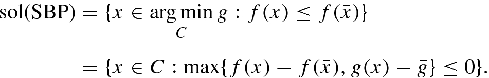
 is a convex function. This shows that
 ,
, 

 is non-increasing and bounded below which establishes the fact that
  is a convergent sequence and hence bounded. This shows that the sequence
  is bounded. In the very next step Solodov [22] uses this boundedness of
  in a profitable way. Let q ≥ 0 be such that
  for all
  .
.


 for all
  . Thus
  is bounded. Now for any
  , the definition i
k tells us that
, the definition i
k tells us that 


 we have


 . Hence from (9.3.14)


 we conclude that {x
k} is also bounded. We can immediately conclude that all accumulation points of {x
k} lie in
we conclude that {x
k} is also bounded. We can immediately conclude that all accumulation points of {x
k} lie in  . Further for any accumulation point x
∗ of
. Further for any accumulation point x
∗ of  we have
  . But this shows that x
∗∈sol(SBP). In fact all accumulation points of
. But this shows that x
∗∈sol(SBP). In fact all accumulation points of  must be in sol(SBP). If x
∗ is an accumulation point of
must be in sol(SBP). If x
∗ is an accumulation point of  , thus there exists a convergent subsequence
  of
of  such that
  as j →∞. Further we have

 (9.3.16) holds, this shows that

 we have
 is strongly convex with modulus ρ > 0 and differentiable, while
  is a convex and differentiable function with ∇g a Lipschitz function on
  with Lipschitz rank (or Lipschitz constant) L > 0. When
  , we are talking about the minimum norm problem. Thus (SBP-1) actually encompasses a large class of important problems.
 . We are already familiar with this reformulation and further they mention that as the Slater condition fails and g
∗ may not be known, the above problem may not be suitable to develop numerical schemes to solve (SBP-1). They mention that even if one could compute g
∗ exactly, the fact that Slater’s condition fails would lead to numerical problems. As a result they take a completely different path by basing their approach on the idea of cutting planes. However we would like to mention that very recently in the thesis of Pandit [18], the above reformulation has been slightly modified to generate a sequence of problems whose solutions converge to that of (SBP) or (SBP-1), depending on the choice of the problem. The algorithm thus presented in the thesis of Pandit [18] has been a collaborative effort with Dutta and Rao and has also been presented in the preprint [19]. The approach in Pandit et al. [19] has been to develop an algorithm where no additional assumption on the upper level objective is assumed other than the fact that it is convex, where the lower level objective is differentiable but need not have a Lipschitz gradient. The algorithm in Pandit [18] or [19] is very simple and just relies on an Armijo type decrease criteria. Convergence analysis has been carried out and numerical experiments have given encouraging results. Further in Pandit et al. [19], the upper level objective need not be strongly convex.
. We are already familiar with this reformulation and further they mention that as the Slater condition fails and g
∗ may not be known, the above problem may not be suitable to develop numerical schemes to solve (SBP-1). They mention that even if one could compute g
∗ exactly, the fact that Slater’s condition fails would lead to numerical problems. As a result they take a completely different path by basing their approach on the idea of cutting planes. However we would like to mention that very recently in the thesis of Pandit [18], the above reformulation has been slightly modified to generate a sequence of problems whose solutions converge to that of (SBP) or (SBP-1), depending on the choice of the problem. The algorithm thus presented in the thesis of Pandit [18] has been a collaborative effort with Dutta and Rao and has also been presented in the preprint [19]. The approach in Pandit et al. [19] has been to develop an algorithm where no additional assumption on the upper level objective is assumed other than the fact that it is convex, where the lower level objective is differentiable but need not have a Lipschitz gradient. The algorithm in Pandit [18] or [19] is very simple and just relies on an Armijo type decrease criteria. Convergence analysis has been carried out and numerical experiments have given encouraging results. Further in Pandit et al. [19], the upper level objective need not be strongly convex.

 be a strictly convex function. Then the Bregman distance generated by h is given as
 and D
h(x, y) = 0 if and only if x = y. Further if h is strongly convex,
and D
h(x, y) = 0 if and only if x = y. Further if h is strongly convex, 
 , then


 , then G
M(x) = ∇g(x), which is thus the source of its name. Further G
M(x
∗) = 0 implies that x
∗ solves the lower level problem in (SBP-1). Further it was shown in [1] that the function
, then G
M(x) = ∇g(x), which is thus the source of its name. Further G
M(x
∗) = 0 implies that x
∗ solves the lower level problem in (SBP-1). Further it was shown in [1] that the function 
 is a minimizer of a convex function
  , then for any
  we have

 denotes the solution set of the problem of minimizing ϕ over
  , then
 , we can immediately eliminate the strict half space
 , the cut at x is given by the hyperplane

 , then
Step 0: Let L > 0 be the Lipschitz constant of ∇g. Let x 0= prox-center of ϕ =
 .
.- Step 1: For k = 1, 2, ⋯where
 and
and

 if
if  and β = 1 if
  .
. when
when  i.e.
i.e.  is that
  and if
  as
as  . These facts are proved in Lemma 2.3 and Lemma 2.4 in Beck and Sabach [1]. In Lemma 2.3 in [1], it is shown that
 , then G
L(x
∗) = 0 and hence
, then G
L(x
∗) = 0 and hence 
 . Since ∇g is Lipschitz continuous with constant L, then from [1] we see that
 , we have

Step 0: Initialization: x 0= prox-center of ϕ =
 . Take L
0 > 0, η > 1.
. Take L
0 > 0, η > 1.- Step 1: For k = 1, 2, ⋯
- (a)Find the smallest non-negative integer i k such that
 and the following inequality
is satisfied. Then set

- (b)Set x k = sol(ϕ, Q k ∩ W k), where

- (a)
 . It has been demonstrated in Lemma 2.5 in Beck and Sabach [1] that if

 .
.
- (a)
{x k} is bounded.
- (b)for any


- (c)
 i.e. x
∗is a solution of (SBP-1). △
i.e. x
∗is a solution of (SBP-1). △

 is a strongly convex function and
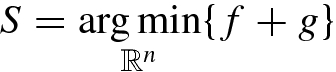
In Sabach and Shtern [20], the following assumptions are made
- (1)
f has Lipschitz-gradient, i.e. ∇f is Lipschitz on
 with Lipschitz constant L
f.
with Lipschitz constant L
f. - (2)
S ≠ ∅.
 , a proper lower semi-continuous prox-mapping is given as


 , whose Lipschitz constant is given as L
ϕ. We are now in a position to state the Big-SAM method.
, whose Lipschitz constant is given as L
ϕ. We are now in a position to state the Big-SAM method.Step 0: Initialization:
![$$ t \in (0, \frac {1}{L_f}] ,\ \beta \in (0, \frac {2}{L_{\phi }+ \rho }) $$](../images/480569_1_En_9_Chapter/480569_1_En_9_Chapter_TeX_IEq209.png) and {α
k} is a sequence satisfying α
k ∈ (0, 1], for all
and {α
k} is a sequence satisfying α
k ∈ (0, 1], for all  ;
;  and
and  and
and  .Set
.Set  as the initial guess solution.
- Step 1: For k = 1, 2, ⋯ , do
- (i)
y k+1 = proxtg(x k − t∇f(x k))
- (ii)
z k+1 = x k − β∇ϕ(x k)
- (iii)
x k+1 = α kz k + (1 − α k)y k.
- (i)
 such that
 solves (SBP-2) and hence
  . Here BiG-SAM means Bilevel gradient sequential averaging method, where the sequential averaging is reflected in (iii) of Step 1 in the above algorithm.
Very recently a modification of the BiG-SAM method was presented in [21].
9.4 Algorithms for Non-smooth Data
 are non-smooth convex functions. The main idea behind the algorithm presented in [23] is to minimize the penalized function
 . As ε ↓ 0, the solutions of the problem
 from the k-th iteration x
k and then update ε
k to ε
k+1 and repeat the step. To realize the descent step Solodov considered the bundle method for unconstrained non-smooth optimization problem (see [16]). Also we will need ε-subdifferential to discuss the algorithm which we present here.
from the k-th iteration x
k and then update ε
k to ε
k+1 and repeat the step. To realize the descent step Solodov considered the bundle method for unconstrained non-smooth optimization problem (see [16]). Also we will need ε-subdifferential to discuss the algorithm which we present here. , is defined as
 is actually a finite subsequence of the finite sequence
  . Let there be l iterations before we choose to modify x
k and ε
k, then k(l) is the index of the last iteration and k = k(l). Let ξ
i ∈ ∂f(y
i) and ζ
i ∈ ∂g(y
i). Then
. Let there be l iterations before we choose to modify x
k and ε
k, then k(l) is the index of the last iteration and k = k(l). Let ξ
i ∈ ∂f(y
i) and ζ
i ∈ ∂g(y
i). Then  . In the bundle method, a linearisation of the function
  is used (see for example [16]). Then
  can be approximated by the following function
 at x
k, which is again a tough job. So the following cutting-planes approximation ψ
l is used by Solodov of the function
at x
k, which is again a tough job. So the following cutting-planes approximation ψ
l is used by Solodov of the function  .
. 
![$$\displaystyle \begin{aligned} \psi_{l}(x):=& \max\limits_{i<l} \{ \varepsilon_k f(x^k) + g(x^k) + \langle \varepsilon_k \xi^i + \zeta^i, x- x^k \rangle\\ & - \varepsilon_k [ f(x^k) - f(y^i) - \langle \xi^i, x^k - y^i \rangle ] - [ g(x^k) - g(y^i) - \langle \zeta^i, x^k - y^i \rangle]\}\\ =& \varepsilon_k f(x^k) + g(x^k) + \max\limits_{i<l} \{ - \varepsilon_k e^{k,i}_{f} - e^{k,i}_{g} + \langle \varepsilon_k \xi^i + \zeta^i, x- x^k \rangle \} \end{aligned}$$](../images/480569_1_En_9_Chapter/480569_1_En_9_Chapter_TeX_Equag.png)


 . Now as ξ
i ∈ ∂f(y
i), for any
. Now as ξ
i ∈ ∂f(y
i), for any  we have
 . Similarly,
  . Then

 is sufficiently small compared with
  , then y
l is considered to be a serious (or acceptable) step and x
k+1 := y
l. In fact y
l is considered to be a serious step if the following decrease criteria holds, i.e.
, then y
l is considered to be a serious (or acceptable) step and x
k+1 := y
l. In fact y
l is considered to be a serious step if the following decrease criteria holds, i.e. 


 at x
k and y
l and also keeps the distance between x
k and y
l into account. Note that δ
l ≥ 0 as
at x
k and y
l and also keeps the distance between x
k and y
l into account. Note that δ
l ≥ 0 as  , which is shown in Lemma 2.1 [23]. If y
l does not satisfy the condition (9.4.7), then y
l is considered as a null step and is not included in the sequence of iterates. But this null step then contributes to construct a better approximation ψ
l+1 of the function
, which is shown in Lemma 2.1 [23]. If y
l does not satisfy the condition (9.4.7), then y
l is considered as a null step and is not included in the sequence of iterates. But this null step then contributes to construct a better approximation ψ
l+1 of the function  using (9.4.3). Then y
l+1 is generated using (9.4.6) with μ
l+1 > 0, which can again be a serious step or a null step. The process is continued until x
k+1 is generated.
using (9.4.3). Then y
l+1 is generated using (9.4.6) with μ
l+1 > 0, which can again be a serious step or a null step. The process is continued until x
k+1 is generated. and another one is aggregate bundle,
  . Both the bundles contain approximated subgradients of the objective functions f and g at x
k and are defined in the following way.
. Both the bundles contain approximated subgradients of the objective functions f and g at x
k and are defined in the following way. 

 are given by (9.4.4) and (9.4.5) and let us set

 and
and  .
. stores the subgradient information of the objective functions at some candidate points y
i. But there may not be any candidate point y
j, j < l such that
stores the subgradient information of the objective functions at some candidate points y
i. But there may not be any candidate point y
j, j < l such that  and
and  . Also note that the construction of
  and
and  justifies the term aggregate bundle. Even though the bundles
  and
and  do not restore all the subgradients at all the candidate points, still a cutting-plane approximation of
  can be done using these bundle information which is given by
 are different. The connection between these two approximations are well established in terms of the solution of the problem given in (9.4.6) and the function (9.4.10) in the following lemma (Lemma 2.1, [23]).


 in Lemma 9.4.1 are obtained as a part of subgradient calculation of ψ
l while solving the strongly convex optimization problem (9.4.6). We have already mentioned that Solodov [23] has developed two different bundles to maintain the bundle size under a fixed limit. Here we discuss how that is done. Let the maximum size that the bundle can attain together be |B|max. So at any l-th step, if
in Lemma 9.4.1 are obtained as a part of subgradient calculation of ψ
l while solving the strongly convex optimization problem (9.4.6). We have already mentioned that Solodov [23] has developed two different bundles to maintain the bundle size under a fixed limit. Here we discuss how that is done. Let the maximum size that the bundle can attain together be |B|max. So at any l-th step, if 
 and the aggregate information
  is included in
  and renamed as
  . Also include
  in
in  and called
  . Now using the bundle information, Solodov constructed the following relations which satisfies all the results mentioned in Lemma 9.4.1.
Step 0: Choose m ∈ (0, 1), an integer
 and β
0 > 0.Set y
0 := x
0 and compute f(y
0), g(y
0), ξ
0 ∈ ∂f(y
0), ζ
0 ∈ ∂g(y
0).Set
and β
0 > 0.Set y
0 := x
0 and compute f(y
0), g(y
0), ξ
0 ∈ ∂f(y
0), ζ
0 ∈ ∂g(y
0).Set  .Define
  and
and 
Step 1: At any l-th step, choose μ l > 0 and compute y l as the solution of (9.4.6) with ψ l, as given in (9.4.10).Compute f(y l), g(y l), ξ l ∈ ∂f(y l), ζ l ∈ ∂g(y l) and
 using (9.4.4) and (9.4.5).
Step 2: If
 , then y
l is a serious step, otherwise null step.
, then y
l is a serious step, otherwise null step.Step 3: Check if
 , otherwise manage the bundle as mentioned earlier.
Step 4: If y l is a serious step, then set x k+1 := y l.Choose 0 < ε k+1 < ε k and 0 < β k+1 < β k. Update
 using (9.4.11).Set k = k + 1 and go to Step 5. If
  , choose 0 < ε
k+1 < ε
k and 0 < β
k+1 < β
k. Set x
k+1 := x
k, k = k + 1 and go to step 5.
, choose 0 < ε
k+1 < ε
k and 0 < β
k+1 < β
k. Set x
k+1 := x
k, k = k + 1 and go to step 5.Step 5: Set l = l + 1 and go to Step 1.
Note that  works as a stopping criteria to minimize the function ψ
k. The convergence result of this algorithm is presented through the following theorem from [23].
works as a stopping criteria to minimize the function ψ
k. The convergence result of this algorithm is presented through the following theorem from [23].
 are convex functions such that f is bounded below on
 and the solution set of the (SBP) problem S is non-empty and bounded. Let us choose μ
l, ε
k, β
ksuch that the following conditions are satisfied at any
and the solution set of the (SBP) problem S is non-empty and bounded. Let us choose μ
l, ε
k, β
ksuch that the following conditions are satisfied at any
 .
. - 1.μ l+1 ≤ μ land there exists
 such that

- 2.
ε k → 0 as k → 0 and
 .
. - 3.
β k → 0 as k → 0.
Then dist(x k, S) → 0 as k → 0. This also implies that any accumulation point of the sequence {x k} is a solution of the (SBP) problem. △
 are continuous, convex functions and
  is closed, convex set. Our algorithm is inspired from the penalisation approach by Solodov [22]. But our algorithm is different from Solodov’s approach in two aspects, one is that we don’t assume any differentiability assumption on the upper and lower level objective functions which naturally helps us to get rid of the Lipschitz continuity assumption on the gradient of the objective functions that is made by Solodov [22], another one is the fact that our algorithm is based on proximal point method whereas Solodov’s algorithm is based on projected gradient method. Our Algorithm is also inspired by Cabot [2] and Facchinei et al. [11] but again different in the sense that our algorithm deals with more general form of (SBP) compared with those. The only assumption we make is that the solution set of the (SBP) problem needs to be non-empty and bounded. This is done to ensure the boundedness of the iteration points which will finally lead to the existence of an accumulation point and hence a solution of the (SBP) problem.
In the proximal point algorithm that we present, we consider an approximate solution rather than the exact solution. For this purpose we need to use ε- subdifferential and ε-normal cone for ε > 0. We have already presented the ε-subdifferential while discussing the last algorithm. Here we present the ε-normal set.
 is defined as


 . Now we present the algorithm formally.
Step 0. Choose x 0 ∈ C, 𝜖 0 ∈ (0, ∞) and let k := 0.
- Step 1. Given x k, λ k > 0, ε k > 0 and η k > 0, choose x k+1 ∈ C such thatwhere

 and
and  .
.
{ε k} is a decreasing sequence such that
 and
and  .
.There exists
 and
and  such that
  for all
  .
. .
.
 be a non-empty closed convex set,
 and
and
 be convex functions. Assume that the functions g and f are bounded below, that the set
 is nonempty, and that the set
 is nonempty and bounded. Let {ε
n}, {λ
n}, {η
n} be nonnegative sequences which satisfy the assumptions mentioned above. Then any sequence {x
n} generated by the algorithm satisfies
is nonempty and bounded. Let {ε
n}, {λ
n}, {η
n} be nonnegative sequences which satisfy the assumptions mentioned above. Then any sequence {x
n} generated by the algorithm satisfies

This also implies that any accumulation point of the sequence {x n}, is a solution of the (SBP) problem. △
The reference [13] in the list of reference was first brought to our notice by M. V. Solodov. In [13], the ε-subgradient is used to develop an inexact algorithmic scheme for the (SBP) problem. however the scheme and convergence analysis developed in [13] is very different from the one in [8]. It is important to note that in contrast to the convergence analysis in [8], the scheme in [13] needs more stringent condition. Also an additional assumption is made on the subgradient of the lower level objective (see Proposition 2, [13]). They also considered the case when the upper level objective is smooth and also has Lipschitz gradient.