You may be asking yourself the question if in the real world you would ever have just one predictor variable; that is, indeed, fair. Most likely, several, if not many, predictor variables or features, as they are affectionately termed in machine learning, will have to be included in your model. And with that, let's move on to multivariate linear regression and a new business case.
In keeping with the water conservation/prediction theme, let's look at another dataset in the alr3 package, appropriately named water. Lately, the severe drought in Southern California has caused much alarm. Even the Governor, Jerry Brown, has begun to take action with a call to citizens to reduce water usage by 20 percent. For this exercise, let's say we have been commissioned by the state of California to predict water availability. The data provided to us contains 43 years of snow precipitation, measured at six different sites in the Owens Valley. It also contains a response variable for water availability as the stream runoff volume near Bishop, California, which feeds into the Owens Valley aqueduct, and eventually, the Los Angeles Aqueduct. Accurate predictions of the stream runoff will allow engineers, planners, and policy makers to plan conservation measures more effectively. The model we are looking to create will consist of the form Y = B0 + B1x1 +...Bnxn + e, where the predictor variables (features) can be from 1 to n.
To begin, we will load the dataset named water and define the structure of the str() function as follows:
> data(water)

> str(water)
'data.frame':   43 obs. of  8 variables:
$ Year   : int  1948 1949 1950 1951 1952 1953 1954 1955 1956 1957 ...
$ APMAM  : num  9.13 5.28 4.2 4.6 7.15 9.7 5.02 6.7 10.5 9.1 ...
$ APSAB  : num  3.58 4.82 3.77 4.46 4.99 5.65 1.45 7.44 5.85 6.13 ...
$ APSLAKE: num  3.91 5.2 3.67 3.93 4.88 4.91 1.77 6.51 3.38 4.08 ...
$ OPBPC  : num  4.1 7.55 9.52 11.14 16.34 ...
$ OPRC   : num  7.43 11.11 12.2 15.15 20.05 ...
$ OPSLAKE: num  6.47 10.26 11.35 11.13 22.81 ...
$ BSAAM  : int  54235 67567 66161 68094 107080 67594 65356 67909 92715 70024 ...
Here we have eight features and one response variable, BSAAM. The observations start in 1943 and run for 43 consecutive years. Since we are not concerned with what year the observations occurred, it makes sense to create a new data frame, excluding the year vector. This is quite easy to do. With one line of code, we can create the new data frame, and then verify that it worked with the head() function as follows:
> socal.water = water[ ,-1] #new dataframe with the deletion of column 1

> head(socal.water)
  APMAM APSAB APSLAKE OPBPC  OPRC OPSLAKE  BSAAM
1  9.13  3.58    3.91  4.10  7.43    6.47  54235
2  5.28  4.82    5.20  7.55 11.11   10.26  67567
3  4.20  3.77    3.67  9.52 12.20   11.35  66161
4  4.60  4.46    3.93 11.14 15.15   11.13  68094
5  7.15  4.99    4.88 16.34 20.05   22.81 107080
6  9.70  5.65    4.91  8.88  8.15    7.41  67594
With all the features being quantitative, it makes sense to look at the correlation statistics and then produce a matrix of scatterplots. The correlation coefficient or Pearson's r, is a measure of both the strength and direction of the linear relationship between two variables. The statistic will be a number between -1 and 1 where -1 is the total negative correlation and +1 is the total positive correlation. The calculation of the coefficient is the covariance of the two variables, divided by the product of their standard deviations. As previously discussed, if you square the correlation coefficient, you will end up with R-squared.
There are a number of ways to produce a matrix of correlation plots. Some prefer to produce
heatmaps, but I am a big fan of what is produced with the corrplot package. It can produce a number of different variations including ellipse, circle, square, number, shade, color, and pie. I prefer the ellipse method, but feel free to experiment with the various methods. Let's load the corrplot package, create a correlation object using the base cor() function, and examine the following results:
> library(corrplot)

> water.cor = cor(socal.water)

> water.cor

                  APMAM      APSAB    APSLAKE      OPBPC
APMAM   1.0000000 0.82768637 0.81607595 0.12238567
APSAB   0.8276864 1.00000000 0.90030474 0.03954211
APSLAKE 0.8160760 0.90030474 1.00000000 0.09344773
OPBPC   0.1223857 0.03954211 0.09344773 1.00000000
OPRC    0.1544155 0.10563959 0.10638359 0.86470733
OPSLAKE 0.1075421 0.02961175 0.10058669 0.94334741
BSAAM   0.2385695 0.18329499 0.24934094 0.88574778
                   OPRC    OPSLAKE     BSAAM
APMAM   0.1544155 0.10754212 0.2385695
APSAB   0.1056396 0.02961175 0.1832950
APSLAKE 0.1063836 0.10058669 0.2493409
OPBPC   0.8647073 0.94334741 0.8857478
OPRC    1.0000000 0.91914467 0.9196270
OPSLAKE 0.9191447 1.00000000 0.9384360
BSAAM   0.9196270 0.93843604 1.0000000
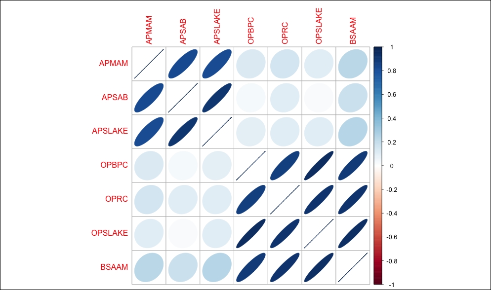
So, what does this tell us? First of all, the response variable is highly and positively correlated with the OP features with OPBPC as 0.8857, OPRC as 0.9196, and OPSLAKE as 0.9384. Also note that the AP features are highly correlated with each other and the OP features as well. The implication is that we may run into the issue of multicollinearity. The correlation plot matrix provides a nice visual of the correlations as follows:
> corrplot(water.cor, method="ellipse")
The output of the preceding code snippet is as follows:
One of the key elements that we will cover here is the very important task of feature selection. In this chapter, we will discuss the best subsets regression methods stepwise, using the leaps package. The later chapters will cover more advanced techniques.
Forward stepwise selection starts with a model that has zero features; it then adds the features one at a time until all the features are added. A selected feature is added in the process that creates a model with the lowest RSS. So in theory, the first feature selected should be the one that explains the response variable better than any of the others, and so on.
Backward stepwise regression begins with all the features in the model and removes the least useful one at a time. A hybrid approach is available where the features are added through forward stepwise regression, but the algorithm then examines if any features that no longer improve the model fit can be removed. Once the model is built, the analyst can examine the output and use various statistics to select the features they believe provide the best fit.
It is important to add here that stepwise techniques can suffer from serious issues. You can perform a forward stepwise on a dataset, then a backward stepwise, and end up with two completely conflicting models. The bottom line is that stepwise can produce biased regression coefficients; in other words, they are too large and the confidence intervals are too narrow (Tibrishani, 1996).
Best subsets regression can be a satisfactory alternative to the stepwise methods for feature selection. In best subsets regression, the algorithm fits a model for all the possible feature combinations; so if you have 3 features, 23 models will be created. As with stepwise regression, the analyst will need to apply judgment or statistical analysis to select the optimal model. Model selection will be the key topic in the discussion that follows. As you might have guessed, if your dataset has many features, this can be quite a task, and the method does not perform well when you have more features than observations (p is greater than n).
Certainly, these limitations for best subsets do not apply to our task at hand. Given its limitations, we will forgo stepwise, but please feel free to give it a try. We will begin by loading the leaps package. In order that we may see how feature selection works, we will first build and examine a model with all the features, then drill down with best subsets to select the best fit.
To build a linear model with all the features, we can again use the lm() function. It will follow the form: fit = lm(y ~ x1 + x2 + x3...xn). A neat shortcut, if you want to include all the features, is to use a period after the tilde symbol instead of having to type them all in. For starters, let's load the leaps package and build a model with all the features for examination as follows:
> library(leaps)

> fit=lm(BSAAM~., data=socal.water)

> summary(fit)

Call:
lm(formula = BSAAM ~ ., data = socal.water)

Residuals:
   Min     1Q Median     3Q    Max
-12690  -4936  -1424   4173  18542

Coefficients:
            Estimate Std. Error t value Pr(>|t|)
(Intercept) 15944.67    4099.80   3.889 0.000416 ***
APMAM         -12.77     708.89  -0.018 0.985725
APSAB        -664.41    1522.89  -0.436 0.665237
APSLAKE      2270.68    1341.29   1.693 0.099112 .
OPBPC          69.70     461.69   0.151 0.880839
OPRC         1916.45     641.36   2.988 0.005031 **
OPSLAKE      2211.58     752.69   2.938 0.005729 **
---
Signif. codes:  0 '***' 0.001 '**' 0.01 '*' 0.05 '.' 0.1 '' 1

Residual standard error: 7557 on 36 degrees of freedom
Multiple R-squared:  0.9248,    Adjusted R-squared:  0.9123
F-statistic: 73.82 on 6 and 36 DF,  p-value: < 2.2e-16
Just like with univariate regression, we examine the p-value on the F-statistic to see if at least one of the coefficients is not zero and, indeed, the p-value is highly significant. We should also have significant p-values for the OPRC and OPSLAKE parameters. Interestingly, OPBPC is not significant despite being highly correlated with the response variable. In short, when we control for the other OP features, OPBPC no longer explains any meaningful variation of the predictor, which is to say that the feature OPBPC adds nothing from a statistical standpoint with OPRC and OPSLAKE in the model.
With the first model built, let's move on to best subsets. We create the sub.fit object using the regsubsets() function of the leaps package as follows:
> sub.fit = regsubsets(BSAAM~., data=socal.water)
Then we create the best.summary object to examine the models further. As with all R objects, you can use the names() function to list what outputs are available, as follows:
> best.summary = summary(sub.fit)

> names(best.summary)
[1] "which"  "rsq"    "rss"    "adjr2"  "cp"     "bic"    "outmat" "obj"
Other valuable functions in model selection include which.min() and which.max(). These functions will provide the model that has the minimum or maximum value respectively, as shown in following code snippet:
> which.min(best.summary$rss)
[1] 6
The code tells us that the model with six features has the smallest RSS, which it should have, as that is the maximum number of inputs and more inputs mean a lower RSS. An important point here is that adding features will always decrease RSS! Furthermore, it will always increase R-squared. We could add a completely irrelevant feature like the number of wins for the Los Angeles Lakers and RSS would decrease and R-squared would increase. The amount would likely be miniscule, but present nonetheless. As such, we need an effective method to properly select the relevant features.
For feature selection, there are four statistical methods that we will talk about in this chapter: Aikake's Information Criterion (AIC), Mallow's Cp (Cp), Bayesian Information Criterion (BIC), and the adjusted R-squared. With the first three, the goal is to minimize the value of the statistic; with adjusted R-squared, the goal is to maximize the statistics value. The purpose of these statistics is to create as parsimonious a model as possible, in other words, penalize model complexity.
The formulation of these four statistics is as follows:
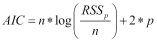 , where
 pis the number of features in the model that we are testing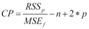 , where
 pis the number of features in the model we are testing andMSEfis the mean of the squared error of the model, with all features included andnis the sample size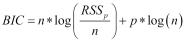 , where
 pis the number of features in the model we are testing andnis the sample size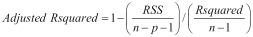 , where
 pis the number of features in the model we are testing andnis the sample size
In a linear model, AIC and Cp are proportional to each other, so we will only concern ourselves with Cp, which follows the output available in the leaps package. BIC tends to select the models with fewer variables than Cp, so we will compare both. To do so, we can create and analyze two plots side by side. Let's do this for Cp followed by BIC with the help of following code snippet:
> par(mfrow=c(1,2))

> plot(best.summary$cp, xlab="number of features", ylab="cp")

> plot(sub.fit, scale="Cp")
The output of preceding code snippet is as follows:
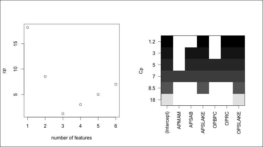
In the plot on the left-hand side, the model with three features has the lowest cp. The plot on the right-hand side displays those features that provide the lowest Cp. The way to read this plot is to select the lowest Cp value at the top of the y axis, which is 1.2. Then, move to the right and look at the colored blocks corresponding to the x axis. Doing this, we see that APSLAKE, OPRC, and OPSLAKE are the features included in this specific model. By using the which.min() and which.max() functions, we can identify how cp compares to BIC and the adjusted R-squared.
> which.min(best.summary$bic)
[1] 3

> which.max(best.summary$adjr2)
[1] 3
In this example, BIC and adjusted R-squared match the Cp for the optimal model. Now, just like with univariate regression, we need to examine the model and test the assumptions. We'll do this by creating a linear model object and examining the plots in a similar fashion to what we did earlier, as follows:
> best.fit = lm(BSAAM~APSLAKE+OPRC+OPSLAKE, data=socal.water)

> summary(best.fit)
Call:
lm(formula = BSAAM ~ APSLAKE + OPRC + OPSLAKE)

Residuals:
   Min     1Q Median     3Q    Max
-12964  -5140  -1252   4446  18649

Coefficients:
            Estimate Std. Error t value Pr(>|t|)
(Intercept)  15424.6     3638.4   4.239 0.000133 ***
APSLAKE       1712.5      500.5   3.421 0.001475 **
OPRC          1797.5      567.8   3.166 0.002998 **
OPSLAKE       2389.8      447.1   5.346 4.19e-06 ***
---
Signif. codes:  0 '***' 0.001 '**' 0.01 '*' 0.05 '.' 0.1 ' ' 1

Residual standard error: 7284 on 39 degrees of freedom
Multiple R-squared:  0.9244,    Adjusted R-squared:  0.9185
F-statistic: 158.9 on 3 and 39 DF,  p-value: < 2.2e-16
With the three-feature model, F-statistic and all the t-tests have significant p-values. Having passed the first test, we can produce our diagnostic plots:
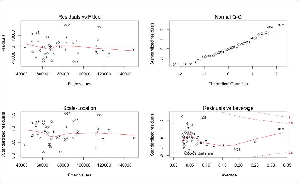
> par(mfrow=c(2,2))

> plot(best.fit)
The output of the preceding code snippet is as follows:
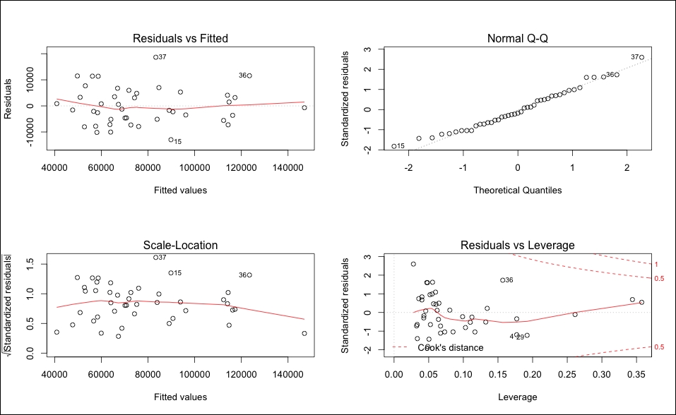
Looking at the plots, it seems safe to assume that the residuals have a constant variance and are normally distributed. There is nothing in the leverage plot that would indicate a requirement for further investigation.
To investigate the issue of collinearity, one can call up the Variance Inflation Factor (VIF) statistic. VIF is the ratio of the variance of a feature's coefficient, when fitting the full model, divided by the feature's coefficient variance when fit by itself. The formula is 1 / (1-R2i), where R2i is the R-squared for our feature of interest, i being regressed by all the other features. The minimum value that the VIF can take is one, which means no collinearity at all. There are no hard and fast rules, but in general, a VIF value that exceeds 5 or 10 indicates a problematic amount of collinearity (James, 2013). A precise value is difficult to select, because there is no hard statistical cut-off point for when multicollinearity makes your model unacceptable.
The vif() function in the car package is all that is needed to produce the values, as can be seen in the following code snippet:
> vif(best.fit)

APSLAKE     OPRC  OPSLAKE
1.011499 6.452569 6.444748
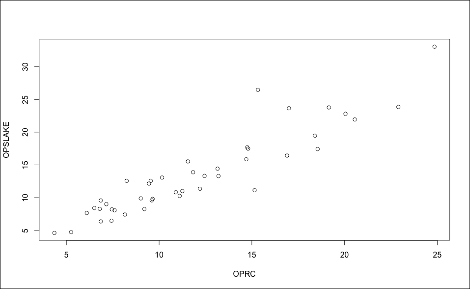
It shouldn't be surprising that we have a potential collinearity problem with OPRC and OPSLAKE (values greater than five) based upon the correlation analysis. A plot of the two variables drives the point home, as seen in the following image:
> plot(socal.water$OPRC, socal.water$OPSLAKE, xlab="OPRC", ylab="OPSLAKE")
The output of preceding command is as follows:
The simple solution to address collinearity is to drop the variables to remove the problem, without compromising the predictive ability. If we look at the adjusted R-squared from the best subsets, we can see that the two-variable model of APSLAKE and OPSLAKE produced a value of 0.90, while adding OPRC only marginally increased it to 0.92:
> best.summary$adjr2 #adjusted r-squared values
[1] 0.8777515 0.9001619 0.9185369 0.9168706 0.9146772 0.9123079
Let's have a look at the two-variable model and test its assumptions, as follows:
> fit.2 = lm(BSAAM~APSLAKE+OPSLAKE, data=socal.water)

> summary(fit.2)

Call:
lm(formula = BSAAM ~ APSLAKE + OPSLAKE)

Residuals:
          Min       1Q   Median       3Q      Max
-13335.8  -5893.2   -171.8   4219.5  19500.2

Coefficients:
                  Estimate Std. Error t value Pr(>|t|)
(Intercept)  19144.9     3812.0   5.022  1.1e-05 ***
APSLAKE       1768.8      553.7   3.194  0.00273 **
OPSLAKE       3689.5      196.0  18.829  < 2e-16 ***
---
Signif. codes:  0 '***' 0.001 '**' 0.01 '*' 0.05 '.' 0.1 ' ' 1

Residual standard error: 8063 on 40 degrees of freedom
Multiple R-squared:  0.9049,    Adjusted R-squared:  0.9002
F-statistic: 190.3 on 2 and 40 DF,  p-value: < 2.2e-16

> par(mfrow=c(2,2))

> plot(fit.2)
The output of the preceding code snippet is as follows:
The model is significant, and the diagnostics do not seem to be a cause for concern. This should take care of our collinearity problem as well and we can check that using the vif() function again as follows:
> vif(fit.2)

 APSLAKE  OPSLAKE
1.010221 1.010221
As I stated previously, I don't believe the plot of fits versus residuals is of concern, but if you have questions, you can formally test the assumption of the constant variance of errors in R. This test is known as the Breusch-Pagan (BP) test. For this, we need to load the lmtest package, and run one line of code. The BP test has the null hypotheses that the error variances are zero versus the alternative of not zero.
> library(lmtest)

> bptest(fit.2)

        studentized Breusch-Pagan test

data:  fit.2
BP = 0.0046, df = 2, p-value = 0.9977
We do not have evidence to reject the null that implies the error variances are zero because p-value = 0.9977. The BP = 0.0046 value in the summary of the test is the chi-squared value.
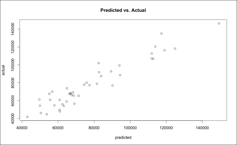
All things considered, it appears that the best predictive model is with the two features APSLAKE and OPSLAKE. The model can explain 90 percent of the variation in the stream runoff volume. To forecast the runoff, it would be equal to 19145 (the intercept) plus 1769 times the measurement at APSLAKE plus 3690 times the measurement at OPSLAKE. A scatterplot of the Predicted vs. Actual values can be done in base R using the fitted values from the model and the response variable values as follows:
> plot(fit.2$fitted.values, socal.water$BSAAM,xlab="predicted", ylab="actual", main="Predicted vs.Actual")
The output of the preceding code snippet is as follows:
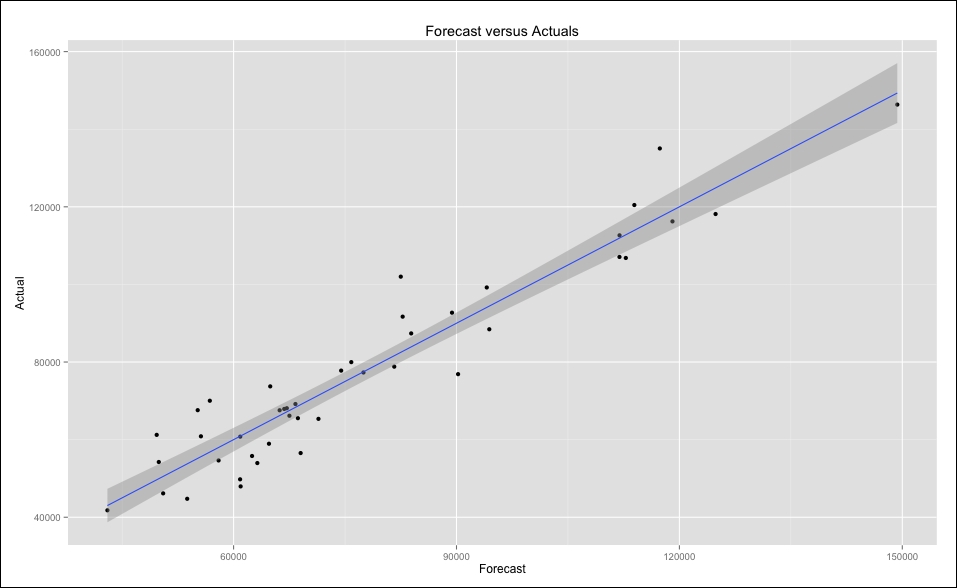
Although informative, the base graphics of R are not necessarily ready for a presentation to be made to business partners. However, we can easily spruce up this plot in R. Several packages to improve graphics are available, and for this example I will use ggplot2. Before producing the plot, we must put the predicted values into our data frame socal.water. I also want to rename BSAAM as Actual, and put in a new vector within the data frame as in the following code snippet:
> socal.water["Actual"] = water$BSAAM #create the vector Actual

> socal.water["Forecast"] = NA #create a vector for the predictions named Forecast, first using NA to create empty observations

> socal.water$Forecast = predict(fit.2) #populate Forecast with the predicted values
Next we will load the ggplot2 package and with one line of code produce a nicer graphic:
> library(ggplot2)

> ggplot(socal.water, aes(x=Forecast, y=Actual)) +geom_point() + geom_smooth(method=lm) + labs(title = "Forecast versus Actuals")
The output of the preceding code snippet is as follows:
Let's examine one final model selection technique before moving on. In the upcoming chapters, we will be discussing cross-validation at some length. Cross-validation is a widely-used and effective method of model selection and testing. Why would this be necessary at all? It comes down to the bias-variance tradeoff. Professor Tarpey of Wright State University has a nice quote on the subject:
"Often we use regression models to predict future observations. We can use our data to fit the model. However, it is cheating to then access how well the model predicts responses using the same data that was used to estimate the model – this will tend to give overly optimistic results in terms of how well a model is able to predict future observations. If we leave out an observation, fit the model and then predict the left out response, then this will give a less biased idea of how well the model predicts".
The cross-validation technique discussed by Professor Tarpey in the preceding quote is known as the
Leave-One-Out-Cross-Validation (LOOCV). In linear models, you can easily perform an LOOCV by examining the
Prediction Error Sum of Squares (PRESS) statistic, and selecting the model that has the lowest value. The R library MPV will calculate the statistic for you, as shown in the following code:
> library(MPV)

> PRESS(best.fit)
 [1] 2426757258

> PRESS(fit.2)
 [1] 2992801411
By this statistic alone, we could select our best.fit model. However, as described previously, I still believe that the more parsimonious model is better in this case. You can build a simple function to calculate the statistic on your own, taking advantage of some elegant matrix algebra as shown in the following code:
> PRESS.best = sum((resid(best.fit)/(1-hatvalues(best.fit)))^2)

> PRESS.fit.2 = sum((resid(fit.2)/(1-hatvalues(fit.2)))^2)

> PRESS.best
[1] 2426757258

> PRESS.fit.2
[1] 2992801411
What are hatvalues, you say? Well, if you take our linear model Y = B0 + B1x + e, we can turn this into a matrix notation: Y = XB + E. In this notation, Y remains unchanged, the X is the matrix of the input values, B is the coefficient, and E represents the errors. This linear model solves for the value of B. Without going into the painful details of matrix multiplication, the regression process yields what is known as a Hat Matrix. This matrix maps, or as some say projects, the calculated values of your model to the actual values; as a result, it captures how influential a specific observation is in your model. So, the sum of the squared residuals divided by one minus hatvalues is the same as LOOCV.