With the data prepared, we will begin the modeling process. For comparison purposes, we will create a model using best subsets regression like the previous two chapters and then utilize the regularization techniques.
The following code is, for the most part, a rehash of what we developed in Chapter 2, Linear Regression – The Blocking and Tackling of Machine Learning. We will create the best subset object using the regsubsets() command and specify the train portion of data. The variables that are selected will then be used in a model on the test set, which we will evaluate with a mean squared error calculation.
The model that we are building is written out as lpsa~. with the tilda and period stating that we want to use all the remaining variables in our data frame with the exception of the response, as follows:
> subfit = regsubsets(lpsa~., data=train)
With the model built, you can produce the best subset with two lines of code. The first one turns the summary model into an object where we can extract the various subsets and determine the best one with the which.min() command. In this instance, I will use BIC, which was discussed in Chapter 2, Linear Regression – The Blocking and Tackling of Machine Learning, which is as follows:
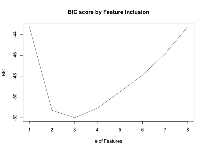
> b.sum = summary(subfit)

> which.min(b.sum$bic)
  [1] 3
The output is telling us that the model with the 3 features has the lowest bic value. A plot can be produced to examine the performance across the subset combinations, as follows:
> plot(b.sum$bic, type="l", xlab="# of Features", ylab="BIC", main="BIC score by Feature Inclusion")
The following is the output of the preceding command:
A more detailed examination is possible by plotting the actual model object, as follows:
> plot(subfit, scale="bic", main="Best Subset Features")
The output of the preceding command is as follows:
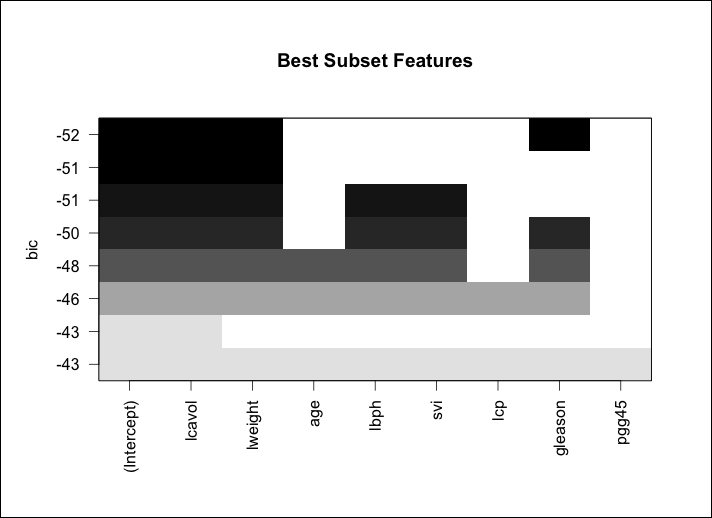
So, the previous plot shows us that the three features included in the lowest BIC are lcavol, lweight, and gleason. It is noteworthy that lcavol is included in every combination of the models. This is consistent with our earlier exploration of the data. We are now ready to try this model on the test portion of the data, but first, we will produce a plot of the fitted values versus the actual values looking for linearity in the solution and as a check on the constancy of the variance. A linear model will need to be created with just the three features of interest. Let's put this in an object called ols for the OLS. Then the fits from ols will be compared to the actuals in the training set, as follows:
> ols = lm(lpsa~lcavol+lweight+gleason, data=train)

> plot(ols$fitted.values, train$lpsa, xlab="Predicted",  ylab="Actual", main="Predicted vs Actual")
The following is the output of the preceding command:
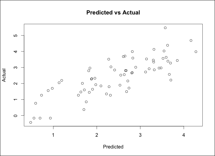
An inspection of the plot shows that a linear fit should perform well on this data and that the nonconstant variance is not a problem. With that, we can see how this performs on the test set data by utilizing the predict() function and specifying newdata=test, as follows:
> pred.subfit = predict(ols, newdata=test)
> plot(pred.subfit, test$lpsa , xlab="Predicted", ylab="Actual", main="Predicted vs Actual")
The values in the object can then be used to create a plot of the Predicted vs Actual values, as shown in the following image:

The plot doesn't seem to be too terrible. For the most part, it is a linear fit with the exception of what looks to be two outliers on the high end of the PSA score. Before concluding this section, we will need to calculate mean squared error (MSE) to facilitate comparison across the various modeling techniques. This is easy enough where we will just create the residuals and then take the mean of their squared values, as follows:
> resid.subfit = test$lpsa - pred.subfit

> mean(resid.subfit^2)
[1] 0.5084126
With ridge regression, we will have all the eight features in the model so this will be an intriguing comparison with the best subsets model. The package that we will use and is in fact already loaded, is glmnet. The package requires that the input features are in a matrix instead of a data frame and for ridge regression, we can follow the command sequence of glmnet(x = our input matrix, y = our response, family = the distribution, alpha=0). The syntax for alpha relates to 0 for ridge regression and 1 for doing LASSO.
To get the train set ready for use in glmnet is actually quite easy using as.matrix() for the inputs and creating a vector for the response, as follows:
> x = as.matrix(train[,1:8])

> y = train[ ,9]
Now, run the ridge regression by placing it in an object called, appropriately I might add, ridge. It is important to note here that the glmnet package will first standardize the inputs before computing the lambda values and then will unstandardize the coefficients. You will need to specify the distribution of the response variable as gaussian as it is continuous and alpha=0 for ridge regression, as follows:
> ridge = glmnet(x, y, family="gaussian", alpha=0)
The object has all the information that we need in order to evaluate the technique. The first thing to try is the print() command, which will show us the number of nonzero coefficients, percent deviance explained, and correspondent value of Lambda. The default number in the package of steps in the algorithm is 100. However, the algorithm will stop prior to 100 steps if the percent deviation does not dramatically improve from one lambda to another, that is, the algorithm converges to an optimal solution. For the purpose of saving space, I will present only the following first five and last ten lambda results:
> print(ridge)

Call:  glmnet(x = x, y = y, family = "gaussian", alpha = 0)

       Df      %Dev    Lambda
  [1,]  8 3.801e-36 878.90000
  [2,]  8 5.591e-03 800.80000
  [3,]  8 6.132e-03 729.70000
  [4,]  8 6.725e-03 664.80000
  [5,]  8 7.374e-03 605.80000
  ...........................
 [91,]  8 6.859e-01   0.20300
 [92,]  8 6.877e-01   0.18500
 [93,]  8 6.894e-01   0.16860
 [94,]  8 6.909e-01   0.15360
 [95,]  8 6.923e-01   0.13990
 [96,]  8 6.935e-01   0.12750
 [97,]  8 6.946e-01   0.11620
 [98,]  8 6.955e-01   0.10590
 [99,]  8 6.964e-01   0.09646
[100,]  8 6.971e-01   0.08789
Look at row 100 for an example. It shows us that the number of nonzero coefficients or—said another way—the number of features included is eight; please recall that it will always be the same for ridge regression. We also see that the percent of deviance explained is .6971 and the Lambda tuning parameter for this row is 0.08789. Here is where we can decide on which lambda to select for the test set. The lambda of 0.08789 can be used, but let's make it a little simpler, and for the test set, try 0.10. A couple of plots might help here so let's start with the package's default, adding annotations to the curve by adding label=TRUE in the following syntax:
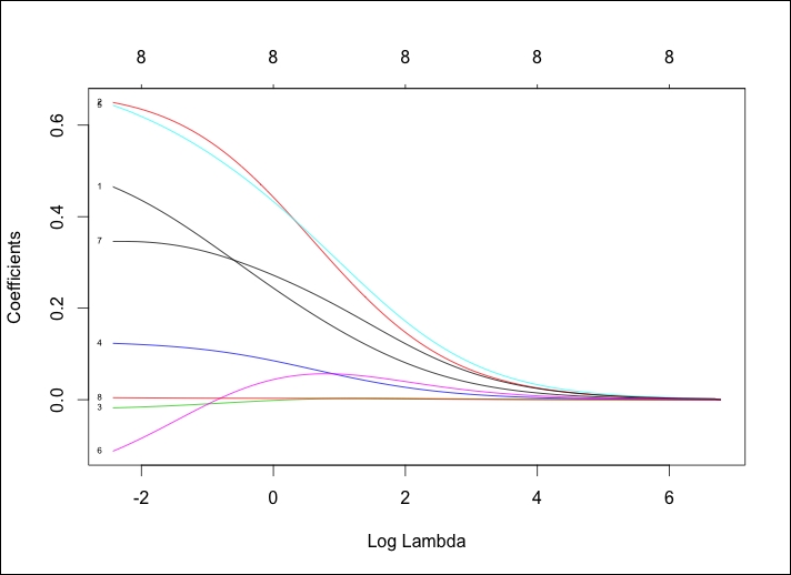
> plot(ridge, label=TRUE)
The following is the output of the preceding command:
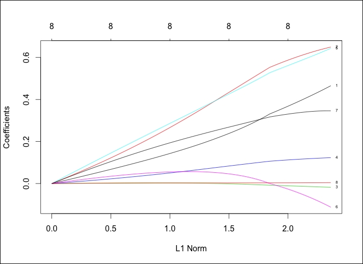
In the default plot, the y axis is the value of Coefficients and the x axis is L1 Norm. The plot tells us the coefficient values versus the L1 Norm. The top of the plot contains a second x axis, which equates to the number of features in the model. Perhaps a better way to view this is by looking at the coefficient values changing as lambda changes. We just need to tweak the code in the following plot() command by adding xvar="lambda". The other option is the percent of deviance explained by substituting lambda with dev.
> plot(ridge, xvar="lambda", label=TRUE)
The output of the preceding command is as follows:
This is a worthwhile plot as it shows that as lambda decreases, the shrinkage parameter decreases and the absolute values of the coefficients increase. To see the coefficients at a specific lambda value, use the coef() command. Here, we will specify the lambda value that we want to use by specifying s=0.1. We will also state that we want exact=TRUE, which tells glmnet to fit a model with that specific lambda value versus interpolating from the values on either side of our lambda, as follows:
> ridge.coef = coef(ridge, s=0.1, exact=TRUE)

> ridge.coef
9 x 1 sparse Matrix of class "dgCMatrix"
                      1
(Intercept)  0.13062197
lcavol       0.45721270
lweight      0.64579061
age         -0.01735672
lbph         0.12249920
svi          0.63664815
lcp         -0.10463486
gleason      0.34612690
pgg45        0.00428580
It is important to note that age, lcp, and pgg45 are close to, but not quite, zero. Let's not forget to plot deviance versus coefficients as well:
> plot(ridge, xvar="dev", label=TRUE)
The output of the preceding command is as follows:
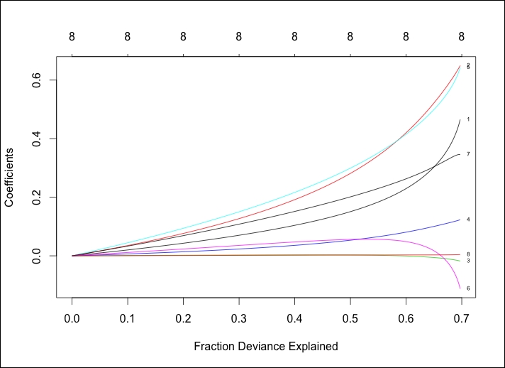
Comparing the two previous plots, we can see that as lambda decreases, the coefficients increase and the percent/fraction of the deviance explained increases. If we would set lambda equal to zero, we would have no shrinkage penalty and our model would equate the OLS.
To prove this on the test set, you will have to transform the features as we did for the training data:
> newx = as.matrix(test[,1:8])
Then, use the predict function to create an object that we will call ridge.y with type = "response" and our lambda equal to 0.10 and plot the Predicted values versus the Actual values, as follows:
> ridge.y = predict(ridge, newx=newx, type="response", s=0.1)

> plot(ridge.y, test$lpsa, xlab="Predicted", ylab="Actual",main="Ridge Regression")
The output of the following command is as follows:
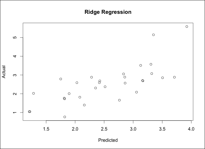
The plot of Predicted versus Actual of Ridge Regression seems to be quite similar to best subsets, complete with two interesting outliers at the high end of the PSA measurements. In the real world, it would be advisable to explore these outliers further so as to understand if they are truly unusual or if we are missing something. This is where domain expertise would be invaluable. The MSE comparison to the benchmark may tell a different story. We first calculate the residuals then take the mean of those residuals squared:
> ridge.resid = ridge.y - test$lpsa

> mean(ridge.resid^2)
[1] 0.4789913
Ridge regression has given us a slightly better MSE. It is now time to put LASSO to the test to see if we can decrease our errors even further.
To run LASSO next is quite simple and we only have to change one number from our ridge regression model, that is, change alpha=0 to alpha=1 in the glmnet() syntax. Let's run this code and also see the output of the model, looking at the first five and last ten results:
> lasso = glmnet(x, y, family="gaussian", alpha=1)

> print(lasso)
Call: glmnet(x = x, y = y, family = "gaussian", alpha = 1)

Df %Dev Lambda
[1,] 0 0.00000 0.878900
[2,] 1 0.09126 0.800800
[3,] 1 0.16700 0.729700
[4,] 1 0.22990 0.664800
[5,] 1 0.28220 0.605800
........................
[60,] 8 0.70170 0.003632
[61,] 8 0.70170 0.003309
[62,] 8 0.70170 0.003015
[63,] 8 0.70170 0.002747
[64,] 8 0.70180 0.002503
[65,] 8 0.70180 0.002281
[66,] 8 0.70180 0.002078
[67,] 8 0.70180 0.001893
[68,] 8 0.70180 0.001725
[69,] 8 0.70180 0.001572
Note that the model building process stopped at step 69 as the deviance explained no longer improved as lambda decreased. Also, note that the Df column now changes along with lambda. At first glance, here it seems that all the eight features should be in the model with a lambda of 0.001572. However, let's try and find and test a model with fewer features, around seven, for argument's sake. Looking at the rows, we see that around a lambda of 0.045, we end up with 7 features versus 8. Thus, we will plug this lambda in for our test set evaluation, as follows:
[31,] 7 0.67240 0.053930
[32,] 7 0.67460 0.049140
[33,] 7 0.67650 0.044770
[34,] 8 0.67970 0.040790
[35,] 8 0.68340 0.037170
Just as with ridge regression, we can plot the results as follows:
> plot(lasso, xvar="lambda", label=TRUE)
The following is the output of the preceding command:
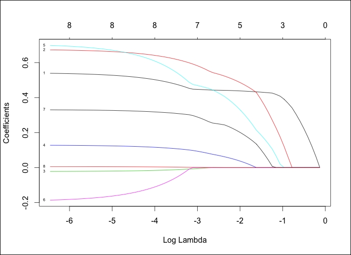
This is an interesting plot and really shows how LASSO works. Notice how the lines labeled 8, 3, and 6 behave, which corresponds to the pgg45, age, and lcp features respectively. It looks as if lcp is at or near zero until it is the last feature that is added. We can see the coefficient values of the seven feature model just as we did with ridge regression by plugging it into coef(), as follows:
> lasso.coef = coef(lasso, s=0.045, exact=TRUE)

> lasso.coef
9 x 1 sparse Matrix of class "dgCMatrix"
                        1
(Intercept) -0.1305852115
lcavol       0.4479676523
lweight      0.5910362316
age         -0.0073156274
lbph         0.0974129976
svi          0.4746795823
lcp          .
gleason      0.2968395802
pgg45        0.0009790322
The LASSO algorithm zeroed out the coefficient for lcp at a lambda of 0.045. Here is how it performs on the test data:
> lasso.y = predict(lasso, newx=newx, type="response", s=0.045)

> plot(lasso.y, test$lpsa, xlab="Predicted", ylab="Actual", main="LASSO")
The output of the preceding command is as follows:
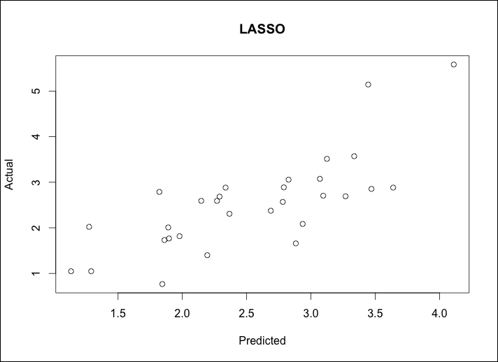
We calculate MSE as we did before:
> lasso.resid = lasso.y - test$lpsa

> mean(lasso.resid^2)
[1] 0.4437209
It looks like we have similar plots as before with only the slightest improvement in MSE. Our last best hope for dramatic improvement is with elastic net. To this end, we will still use the glmnet package. The twist will be that we will solve for lambda and for the elastic net parameter known as alpha. Recall that alpha = 0 is the ridge regression penalty and alpha = 1 is the LASSO penalty. The elastic net parameter will be 0 ≤ alpha ≤ 1. Solving for two different parameters simultaneously can be complicated and frustrating but we can use our friend in R, the caret package, for assistance.
The caret package stands for classification and regression training. It has an excellent companion website to help in understanding all of its capabilities: http://topepo.github.io/caret/index.html. The package has many different functions that you can use and we will revisit some of them in the later chapters. For our purpose here, we want to focus on finding the optimal mix of lambda and our elastic net mixing parameter, alpha. This is done using the following simple three-step process:
- Use the
expand.grid()function in base R to create a vector of all the possible combinations of alpha and lambda that we want to investigate. - Use the
trainControl()function from thecaretpackage to determine the resampling method; we will use LOOCV as we did in Chapter 2, Linear Regression – The Blocking and Tackling of Machine Learning. - Train a model to select our alpha and lambda parameters using
glmnet()in caret'strain()function.
Once we've selected our parameters, we will apply them to the test data in the same way as we did with ridge regression and LASSO. Our grid of combinations should be large enough to capture the best model but not too large that it becomes computationally unfeasible. That won't be a problem with this size dataset, but keep this in mind for future references. I think we can do the following:
- alpha from
0to1by0.2increments; remember that this is bound by0and1 - lambda from
0.00to0.2in steps of0.02; the0.2lambda should provide a cushion from what we found in ridge regression (lambda=0.1) and LASSO (lambda=0.045)
You can create this vector using the expand.grid() function and building a sequence of numbers for what the caret package will automatically use. The caret package will take the values for alpha and lambda with the following code:
> grid = expand.grid(.alpha=seq(0,1, by=.2), .lambda=seq(0.00,0.2, by=0.02))
The table() function will show us the complete set of 66 combinations:
> table(grid)
      .lambda
.alpha 0 0.02 0.04 0.06 0.08 0.1 0.12 0.14 0.16 0.18 0.2
   0   1    1    1    1    1   1    1    1    1    1   1
   0.2 1    1    1    1    1   1    1    1    1    1   1
   0.4 1    1    1    1    1   1    1    1    1    1   1
   0.6 1    1    1    1    1   1    1    1    1    1   1
   0.8 1    1    1    1    1   1    1    1    1    1   1
   1   1    1    1    1    1   1    1    1    1    1   1
We can confirm that this is what we wanted—alpha from 0 to 1 and lambda from 0 to 0.2. For the resampling method, we will put in the code for LOOCV for the method. There are other resampling alternatives such as bootstrapping or k-fold cross-validation and numerous options that you can use with trainControl(), but we will explore this options in future chapters. You can tell the model selection criteria with selectionFunction() in trainControl(). For quantitative responses, the algorithm will select based on its default of Root Mean Square Error (RMSE), which is perfect for our purposes:
> control = trainControl(method="LOOCV")
It is now time to use train() to determine the optimal elastic net parameters. The function is similar to lm(). We will just add the syntax: method="glmnet", trControl=control and tuneGrid=grid. Let's put this in an object called enet.train:
> enet.train = train(lpsa~., data=train, method="glmnet", trControl=control, tuneGrid=grid)
Calling the object will tell us the parameters that lead to the lowest RMSE, as follows:
> enet.train
glmnet

67 samples
 8 predictor

No pre-processing
Resampling:

Summary of sample sizes: 66, 66, 66, 66, 66, 66, ...

Resampling results across tuning parameters:

  alpha  lambda  RMSE   Rsquared
  0.0    0.00    0.750  0.609
  0.0    0.02    0.750  0.609
  0.0    0.04    0.750  0.609
  0.0    0.06    0.750  0.609
  0.0    0.08    0.750  0.609
  0.0    0.10    0.751  0.608
   .........................
  1.0    0.14    0.800  0.564
  1.0    0.16    0.809  0.558
  1.0    0.18    0.819  0.552
  1.0    0.20    0.826  0.549
RMSE was used to select the optimal model using the smallest value. The final values used for the model were alpha = 0 and lambda = 0.08.
This experimental design has led to the optimal tuning parameters of alpha = 0 and lambda = 0.08, which is a ridge regression with s=0.08 in glmnet, recall that we used 0.10. The R-squared is 61 percent, which is nothing to write home about.
The process for the test set validation is just as before:
> enet = glmnet(x, y,family="gaussian", alpha=0, lambda=.08)

> enet.coef = coef(enet, s=.08, exact=TRUE)

> enet.coef
9 x 1 sparse Matrix of class "dgCMatrix"
                       1
(Intercept)  0.137811097
lcavol       0.470960525
lweight      0.652088157
age         -0.018257308
lbph         0.123608113
svi          0.648209192
lcp         -0.118214386
gleason      0.345480799
pgg45        0.004478267

> enet.y = predict(enet, newx=newx, type="response", s=.08)

> plot(enet.y, test$lpsa, xlab="Predicted", ylab="Actual", main="Elastic Net")
The output of the preceding command is as follows:
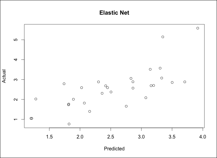
Calculate MSE as we did before:
> enet.resid = enet.y – test$lpsa

> mean(enet.resid^2)
[1] 0.4795019
This model error is similar to the ridge penalty. On the test set, our LASSO model did the best in terms of errors. We may be over-fitting! Our best subset model with three features is the easiest to explain, and in terms of errors, is acceptable to the other techniques. We can use a 10-fold cross-validation in the glmnet package to possibly identify a better solution.
We have used LOOCV with the caret package; now we will try k-fold cross-validation. The glmnet package defaults to ten folds when estimating lambda in cv.glmnet(). In k-fold CV, the data is partitioned into an equal number of subsets (folds) and a separate model is built on each k-1 set and then tested on the corresponding holdout set with the results combined (averaged) to determine the final parameters. In this method, each fold is used as a test set only once. The glmnet package makes it very easy to try this and will provide you with an output of the lambda values and the corresponding MSE. It defaults to alpha = 1, so if you want to try ridge regression or an elastic net mix, you will need to specify it. As we will be trying for as few input features as possible, we will stick to the default:
> set.seed(317)

> lasso.cv = cv.glmnet(x, y)

> plot(lasso.cv)
The output of the preceding code is as follows:
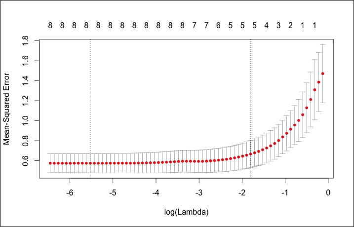
The plot for CV is quite different than the other glmnet plots, showing log(Lambda) versus Mean-Squared Error along with the number of features. The two dotted vertical lines signify the minimum of MSE (left line) and one standard error from the minimum (right line). One standard error away from the minimum is a good place to start if you have an over-fitting problem. You can also call the exact values of these two lambdas, as follows:
> lasso.cv$lambda.min #minimum
[1] 0.003985616

> lasso.cv$lambda.1se #one standard error away
[1] 0.1646861
Using lambda.1se, we can go through the following process of viewing the coefficients and validating the model on the training data:
> coef(lasso.cv, s ="lambda.1se")
9 x 1 sparse Matrix of class "dgCMatrix"
                     1
(Intercept) 0.04370343
lcavol      0.43556907
lweight     0.45966476
age         .
lbph        0.01967627
svi         0.27563832
lcp         .
gleason     0.17007740
pgg45       .

> lasso.y.cv = predict(lasso.cv, newx=newx, type="response", s="lambda.1se")

> lasso.cv.resid = lasso.y.cv - test$lpsa


> mean(lasso.cv.resid^2)
[1] 0.4559446
This model achieves an error of 0.46 with just five features, zeroing out age, lcp, and pgg45.