To start, we will load these three packages. The data is in the MASS package, but this is a required dependent package loaded with neuralnet:
> library(caret)

> library(neuralnet)
Loading required package: grid
Loading required package: MASS

> library(vcd)
The neuralnet package will be used for the building of the model and caret for the data preparation. The vcd package will assist us in data visualization. Let's load the data and examine its structure:
> data(shuttle)

> str(shuttle)
'data.frame':256 obs. of  7 variables:
 $ stability: Factor w/ 2 levepicels "stab","xstab": 2 2 2 2 2 2 2 2 2 2 ...
 $ error    : Factor w/ 4 levels "LX","MM","SS",..: 1 1 1 1 1 1 1 1 1 1 ...
 $ sign     : Factor w/ 2 levels "nn","pp": 2 2 2 2 2 2 1 1 1 1 ...
 $ wind     : Factor w/ 2 levels "head","tail": 1 1 1 2 2 2 1 1 1 2 ...
 $ magn     : Factor w/ 4 levels "Light","Medium",..: 1 2 4 1 2 4 1 2 4 1 ...
 $ vis      : Factor w/ 2 levels "no","yes": 1 1 1 1 1 1 1 1 1 1 ...
 $ use      : Factor w/ 2 levels "auto","noauto": 1 1 1 1 1 1 1 1 1 1 ...
The data consists of 256 observations and 7 variables. Notice that all of the variables are categorical and the response is use with two levels, auto and noauto. The covariates are as follows:
stability: This is stable positioning or not (stab/xstab)error: This is the size of the error (MM/SS/LX)sign: This is the sign of the error, positive or negative (pp/nn)wind: This is thewindsign (head/tail)magn: This is thewindstrength (Light/Medium/Strong/Out of Range)vis: This is the visibility (yes/no)
We will build a number of tables to explore the data, starting with the response/outcome:
> table(shuttle$use)

  auto noauto
   145    111
Almost 57 percent of the time, the decision is to use the autolander. There are a number of possibilities to build tables for categorical data. The table() function is perfectly adequate to compare one versus another, but if you add a third, it can turn into a mess to look at. The vcd package offers a number of table and plotting functions. One is structable(). This function will take a formula (column1 + column2 ~ column3), where column3 becomes the rows in the table:
> table1=structable(wind+magn~use, shuttle)

> table1
       wind  head                    tail
       magn Light Medium Out Strong Light Medium Out Strong
use
auto           19     19  16     18    19     19  16     19
noauto         13     13  16     14    13     13  16     13
Here, we can see that in the cases of a headwind that was Light in magnitude, auto occurred 19 times and noauto, 13 times. The vcd package offers the mosaic() function to plot the table created by structable() and provide the p-value for a chi-squared test:
> mosaic(table1, gp=shading_hcl)
The output of the preceding command is as follows:
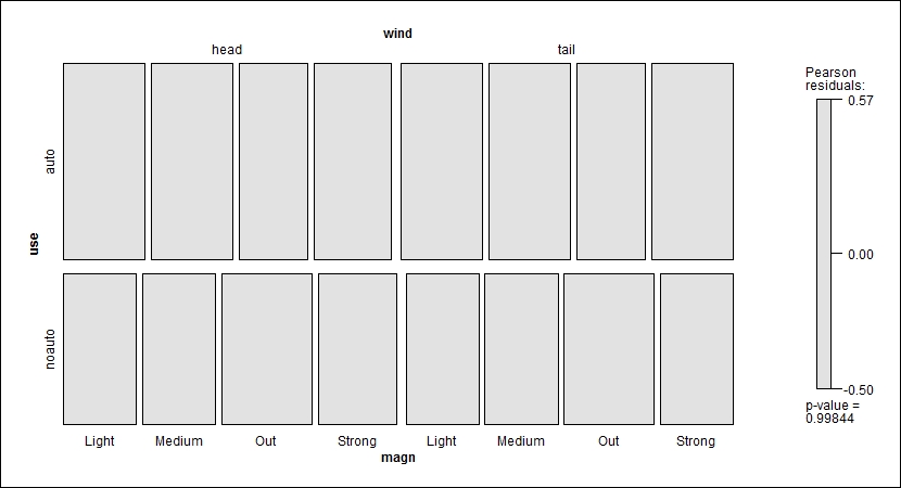
The plot tiles correspond to the proportional size of their respective cells in the table, created by recursive splits. You can also see that the p-value is not significant, so the variables are independent, which means that knowing the levels of wind and/or magn does not help us predict the use of the autolander. You do not need to include a structable() object in order to create the plot as it will accept a formula just as well. We will also drop the shading syntax, which drops the colored shading and residuals bar on the right. This can make for a cleaner plot:
> mosaic(use~error+vis, shuttle)
The output of the preceding command is as follows:
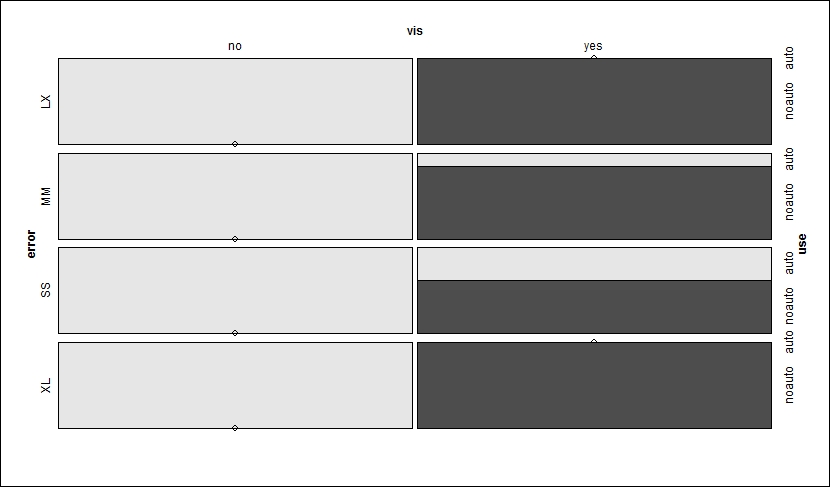
Note that the shading of the table has changed, reflecting the rejection of the null hypothesis and dependence in the variables. The plot first takes and splits the visibility. The result is that if the visibility is no, then the autolander is used. The next split is horizontal by error. If error is SS or MM when vis is no, then the autolander is recommended, otherwise it is not. A p-value is not necessary as the gray shading indicates significance.
One can also examine proportional tables with the prop.table() function as a wrapper around table():
> table(shuttle$use, shuttle$stability)

         stab xstab
  auto     81    64
  noauto   47    64

> prop.table(table(shuttle$use, shuttle$stability))

              stab     xstab
  auto   0.3164062 0.2500000
  noauto 0.1835938 0.2500000
In case we forget, the chi-squared tests are quite simple:
> chisq.test(shuttle$use, shuttle$stability)

Pearson's Chi-squared test with Yates' continuity
correction

data:  shuttle$use and shuttle$stability
X-squared = 4.0718, df = 1, p-value = 0.0436
Preparing the data for a neural network is very important as all the covariates and responses need to be numeric. In our case, we have all of them categorical. The caret package allows us to quickly create dummy variables as our input features:
> dummies = dummyVars(use~.,shuttle, fullRank=TRUE)

> dummies
Dummy Variable Object

Formula: use ~ .
7 variables, 7 factors
Variables and levels will be separated by '.'
A full rank encoding is used
To put this into a data frame, we need to predict the dummies object to an existing data, either the same or different, in as.data.frame(). Of course, the same data is needed here:
> shuttle.2 = as.data.frame(predict(dummies, newdata=shuttle))

> names(shuttle.2)
 [1] "stability.xstab" "error.MM"        "error.SS"
 [4] "error.XL"        "sign.pp"         "wind.tail"
 [7] "magn.Medium"     "magn.Out"        "magn.Strong"
[10] "vis.yes"

> head(shuttle.2)
  stability.xstab error.MM error.SS error.XL sign.pp wind.tail
1               1        0        0        0       1         0
2               1        0        0        0       1         0
3               1        0        0        0       1         0
4               1        0        0        0       1         1
5               1        0        0        0       1         1
6               1        0        0        0       1         1
  magn.Medium magn.Out magn.Strong vis.yes
1           0        0           0       0
2           1        0           0       0
3           0        0           1       0
4           0        0           0       0
5           1        0           0       0
6           0        0           1       0
We now have an input feature space of ten variables. Stability is now either 0 for stab or 1 for xstab. Base error is LX and three variables represent the other categories.
The response can be created using the ifelse() function:
> shuttle.2$use = ifelse(shuttle$use=="auto",1,0)

> table(shuttle.2$use)

  0   1
111 145
The caret package also provides us with a functionality to create the train and test sets. The idea is to index each observation as train or test and then split the data accordingly. Let's do this with a 70/30 train to test split, as follows:
> set.seed(123)

> trainIndex = createDataPartition(shuttle.2$use, p = .7, list = FALSE, times = 1)

> head(trainIndex)
     Resample1
[1,]         1
[2,]         2
[3,]         6
[4,]         9
[5,]        10
[6,]        11
The values in trainIndex provide us with a row number; in our case, 70 percent of the total row numbers in shuttle.2. It is now a simple case of creating the train/test datasets and to make sure that the response variable is balanced between them.
> shuttleTrain = shuttle.2[ trainIndex,]

> shuttleTest  = shuttle.2[-trainIndex,]

> table(shuttleTrain$use)

 0  1
81 99
> table(shuttleTest$use)

 0  1
30 46
Nicely done! We are now ready to begin building the neural networks.