For this analysis, we will only need to load two packages as well as the Groceries dataset:
> library(arules)

> library(arulesViz)

> data(Groceries)
> head(Groceries)
> str(Groceries)
> Groceries
transactions in sparse format with
 9835 transactions (rows) and
 169 items (columns)
This dataset is structured as a sparse matrix object known as the class of transaction.
So, once the structure is that of the class transaction, our standard exploration techniques will not work, but the arules package offers us other techniques to explore the data. On a side note, if you have a data frame or matrix and want to convert it to the transaction class, you can do this with a simple syntax using the as() function. The following code is for illustrative purposes only, so do not run it:
> transaction.class.name = as(current.data.frame,"transactions")
The best way to explore this data is with an item frequency plot using the itemFrequencyPlot() function in the arules package. You will need to specify the transaction dataset, the number of items with the highest frequency to plot, and whether or not you want the relative or absolute frequency of the items. Let's first look at the absolute frequency and the top 10 items only:
> itemFrequencyPlot(Groceries,topN=10,type="absolute")
The output of the preceding command is as follows:
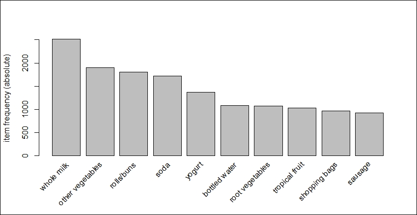
The top item purchased was whole milk with roughly 2,500 of the 9,836 transactions in the basket. For a relative distribution of the top 15 items, let's run the following code:
> itemFrequencyPlot(Groceries,topN=15)
The following is the output of the preceding command:
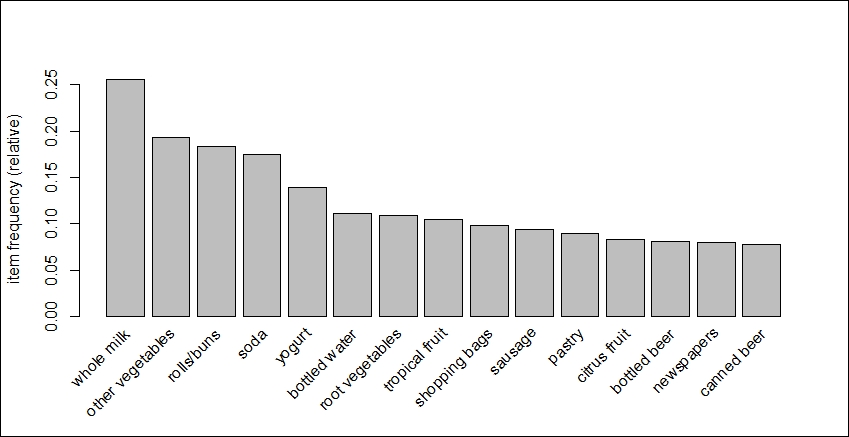
Alas, here we see that beer shows up as the 13th and 15th most purchased item at this store. Just under 10 percent of the transactions had purchases of bottled beer and/or canned beer.
For the purposes of this exercise, this is all we really need to do, and therefore, we can move right on to the modeling and evaluation.