 j=1,2,…,h (1)
In this article, a classification framework that uses quantum-behaved particle swarm optimization neural network (QPSONN) classifiers for diagnosing a disease is discussed. The neural network used for classification is radial basis function neural network (RBFNN). For training the RBFNN K-means clustering algorithm and quantum-behaved particle swarm optimization (QPSO) algorithm has been used. The K-means clustering algorithm is used to find the optimal number of clusters which determines the number of neurons in the hidden layer. The cluster approximation error is used to find the optimal clusters. The weights between the hidden and the output layer is determined using QPSO algorithm based on the mean squared error (MSE). The performance of the developed classifier model has been tested with five clinical datasets, namely Pima Indian Diabetes, Hepatitis, Bupa Liver Disease, Wisconsin Breast Cancer and Cleveland Heart Disease were obtained from the University of California, Irvine (UCI) machine learning repository.
Clinical decision making is a pervasive task that needs to be accurate. Knowledge models extracted from medical data should be novel, interesting and comprehensible to clinicians. Data mining techniques have been widely used in Computer Aided Diagnosis (CAD) systems, because of their ability to discover hidden patterns and relationships to solve the diagnostic problems in medical data (Sadoughi, Ghaderzadeh, Fein, & Standring, 2014). The common data mining tasks are association rule mining, clustering and classification (Han & Kamber, 2000). Association rule mining is a process of finding frequent patterns, associations, correlation among sets of items in transaction databases, relational databases and other information repositories. Clustering is a process of finding similarities between data according to the characteristics found in the data and grouping similar data objects into clusters. Classification is a supervised machine learning technique and is carried out in two steps namely learning and classification. In the learning step the classification model is constructed. In the classification step the constructed model is used to classify the test samples.
To address the problem of classification, the commonly used approaches are Artificial Neural Network (ANN), Decision trees, Support Vector Machine (SVM), Bayesian classifiers and K-Nearest Neighbor classifiers (Neelamegam & Ramaraj, 2013). Researchers have also developed hybrid classifiers to address the classification problem in clinical datasets and microarray gene expression data. A hybrid classifier for classifying leukemia gene expression data is presented in (Susmi, Nehemiah, Kannan, & Christopher, 2015). Mokeddem and Baghdad, (2016) performed an assessment for predicting coronary heart disease using fuzzy logic based clinical decision support system. Dasarathy and Sheela, (1979) introduced an ensemble based classification system. This system partitions the feature space into two or more classifiers. In 1990, Hansen and Salamon proved the generalization performance of a neural network that can be improved using an ensemble based neural network.
ANNs are computational models inspired by the biological nervous system (De Castro, 2006). Radial Basis Function (RBF) network is a feedforward ANN introduced by Broomhead and Lowe (Broomhead & Lowe, 1988). RBF network has several advantages when compared to the other types of ANNs, such as their simple structure, good approximation capabilities and faster learning rate (Qasem, Shamsuddin, Hashim, Darus, & Al-Shammari, 2013). Because of the above capabilities, the RBFNN can be applied in many science and engineering domains, such as function approximation, time series prediction, curve fitting, control and classification problems (Devaraj, Yegnanarayana, & Ramar, 2002; Du & Zhai, 2008; Fu & Wang, 2003; Han & Xi, 2004; Oyang, Hwang, Ou, Chen, & Chen, 2005).
RBFNN has three functional layers, namely input layer, hidden layer and output layer. The neurons in the input layer represent the input features. The hidden layer performs fixed nonlinear transformations of the input features and the connections from the input layer to hidden layer are not weighted. The RBFNN training is a two phase training process. In the first phase of training, number of neurons in the hidden layer is determined. In the second phase, the optimal weights between the hidden and the output layer is determined. In the first phase, finding the number of neurons in the hidden layer plays a major role in classification, as it affects the generalization and complexity of the network. If the number of neurons in the hidden layer is too high, an overfitting of the network may occur and if the number of neurons in the hidden layer is low underfitting of the network may occur. Training radial basis function neural network using particle swarms (Liu, Zheng, Shi, & Chen, 2004) achieves more rational architecture for RBFNN. Hien and Huan (2015) used the training function as multivariate regression function to train the RBFNN. Training function uses grid equally spaced nodes to find the number of neurons in the hidden layer and the suitable position of centers in each hidden neuron. To train the weights between the hidden and the output layer of the RBFNN exact interpolation algorithm is used.
Finding optimal centers of hidden neurons in hidden layer is important for classification (Simon, 2002). If the centers of the RBF units are chosen randomly, the input shifts away from the connection weights, which in turn affects the RBFN network performance. The non-linear activation functions in hidden layer namely, Gaussian, multiquadric, inverse multiquadric, inverse quadratic, thin plate spline and Cauchy are used (Antonie, Zaiane & Holte, 2006). The activation function used in this work is Gaussian function. In Gaussian function, the width parameter controls the behavior of the function, where the larger width implies less sensitivity of the network. Therefore, optimization of the width parameter in each neuron, is included in the training procedure. The output layer performs the (linear) summation functions and the connections are weighted (Leonard & Kramer, 1991). These weights are determined based on the mean squared error of the network.
Researchers had developed many algorithms for the first phase training of RBFNN, such as sub sampling technique (Orr, 1996), unsupervised learning (Tarassenko & Roberts, 1994) and Gradient descent method (Karayiannis, 1997). In sub sampling technique, the centers are chosen randomly from the input data points. Clustering technique comes under unsupervised learning, which results in grouping of objects where the intra-cluster variation must be less and the inter-cluster variation must be high. In Gradient descent method, the centers are fixed and the weights are updated, which minimizes the squared error. The second phase training of RBFNN uses algorithms such as Kalman filtering (KF) (Simon, 2002) and Gradient-Descent (GD) (Karayiannis, 1999) algorithm. These two training algorithms suffers from slower convergence due to local minima problem and increasing training time which is used to find the optimal gradient. To overcome the above limitations, several global optimization algorithms with single error function can be used to solve the training problems of RBFNN. The global optimization algorithms such as genetic algorithms (GA) (Barreto, Barbosa, & Ebecken, 2002), artificial immune system (AIS) (De Castro & Von Zuben, 2001), particle swarm optimization (PSO) (Liu et al., 2004), differential evolution (DE) (Yu & He, 2006) and Artificial Bee Colony (ABC) (Kurban & Beşdok, 2009) are used for training RBFNN.
In this research, a CAD system is developed that uses a QPSONN classification model for diagnosing a particular disease. In QPSONN model, the determination of the number of neurons in the hidden layer is computed using the k-means clustering algorithm (Hartigan & Wong, 1979). Based on Euclidean distance, the algorithm clusters the input data points. The clustering is performed by minimizing the sum of squared distances between the input data and the corresponding centroid. The optimal number of clusters is chosen based on the cluster error. These clusters serve as the hidden nodes in the hidden layer. The output of the hidden neuron is obtained using the cluster center. The weights between the hidden and the output layer is optimized using QPSO algorithm based on the MSE of the QPSONN classifier. This QPSONN classifier is tested with five clinical datasets namely PID, WBC and CHD obtained from the University of California, Irvine (UCI) machine learning repository. The performance of the QPSONN classifier model is compared with different classification methods in the literature for all datasets. The experimental results show that the efficiency of the developed classifier is dominant in terms of classification accuracy when compared to other methods.
Related works carried out by researchers using the clinical datasets from the UCI machine learning repository are discussed below.
Abbass (2001) in their work, had presented an Evolutionary Artificial Neural Network (EANN) based on Pareto multi-objective optimization and differential evolution (DE) with local search called Memetic Pareto Artificial Neural Networks (MPANN). Their work had two objectives namely, minimize the error and determine the number of hidden neurons. The tradeoffs between the two objectives were used to set the networks with different number of hidden units. The algorithm will return two pareto networks with the same number of hidden units. If the number of parents is less than three, then the pareto optimal solutions are removed from the population and the population is reevaluated. The disadvantage of EANN is slow training. The MPANN overcomes the disadvantage of EANN with higher accuracy. This model was tested with PID and WBC dataset obtained from the UCI machine learning repository, and it achieves 74.90% and 98.10% accuracy for the above datasets respectively.
Goh, Teoh, and Tan (2008) have presented a multiobjective EANN for optimizing the ANN structure. In this work, the hidden layer neurons are estimated using a geometrical measure based on singular value decomposition (SVD). The features of a variable representation in multiobjective approach provides easy adaptation in neural network structures. This procedure adapts the number of necessary neurons in the hidden layer based on the geometrical measure. The adaptive local search intensity scheme had been used for local fine-tuning of the ANN structure. This approach was tested with seven datasets among which five datasets were clinical datasets, namely WBC, PID, CHD, hepatitis and Bupa liver obtained from the UCI machine learning repository. This hybrid optimization method achieves 96.3%, 78.50%, 79.70%, 80.3% and 68.0% accuracy for above datasets respectively.
Cai, Chen, and Zhang, (2010) have proposed a multiobjective simultaneous learning framework for clustering and classification (MSCC) of datasets. This MSCC uses multiple objective functions to solve the classification and clustering problems simultaneously. The cluster center performs the role of a bridge connecting the clustering and classification. This cluster center is embedded with the objective functions for giving effective clustering and classification solutions simultaneously. This method was experimented on 17 datasets obtained from the UCI machine learning repository, out of which four are clinical datasets, namely WBC, PID, CHD and Bupa liver. The accuracy of this method is 97.60%, 76.50%, 84.2% and 68.20% for breast cancer, diabetes, heart disease and liver datasets respectively.
Qasem and Shamsuddin, (2011) have introduced a time variant multi-objective particle swarm optimization (TVMOPSO) of radial basis function (RBF) network for diagnosing diseases. In this work, the TVMOPSO algorithm determines the set of connection centers and weights of the RBFNN based on the accuracy of the RBFNN-TVMOPSO classifier. This classifier was tested on three clinical datasets, namely WBC, PID and Hepatitis obtained from the UCI machine learning repository. This method achieves 96.53%, 78.02% and 82.26% accuracy for Wisconsin breast cancer, Pima Indian diabetes and Hepatitis datasets respectively.
Leung, Tang, and Wong, (2012) have presented a hybrid particle swarm optimization for training the neural networks. In this model, a modified fisher ratio class separability measure (MFRCSM) is used to decrease the inertia weights linearly of each particle. The MFRCSM was used to create number of nodes in the hidden layer. The orthogonal least square algorithm (OLSA) was used to optimize the structure of the RBFNN including the weights and the controlling parameters. This method was tested with eight benchmark datasets among which three datasets are clinical datasets namely, WBC, PID and heart disease obtained from the UCI machine learning repository. This method achieves 95.78%, 79.66% and 86.79% accuracy for the above datasets respectively.
Qasem et al., (2013) had presented a multiobjective particle swarm optimization with local search features and was applied to design a radial basis function (RBF) network (MPSON) design. This model was compared with the memetic non-dominated sorting genetic algorithm based RBF network (MGAN). It was used to optimize the RBF network structure for improving the accuracy. The two algorithms was tested on twelve datasets for classification among which six datasets were clinical datasets, namely WBC, PID, CHD, Hepatitis, Bupa liver and lung cancer dataset obtained from the UCI machine learning repository. This approach achieved 97.97%, 83.88%, 87.15%, 88%, 78.78% and 78.68% accuracy for the above datasets respectively.
Mangat and Vig (2014) in their work, have proposed a rule mining classifier based on a dynamic particle swarm optimizer (DP-AC). Seeding procedure is based on the concept of regions and their regrouping. It does not allow premature convergence but gives a better convergence value in every dimension. This DP-AC method was tested on clinical datasets, namely, Dermatology, Thyroid, CHD, Hepatitis, Bupa liver, PID, Parkinsons and SPECTF heat from the UCI machine learning repository, and it achieves 92.25%, 96.62%, 56.50%, 84.33%, 61.86%, 74.11%, 87.00% and 84.45% accuracy for above datasets respectively.
Bhardwaj and Tiwari (2015) presented Breast Cancer diagnosis using genetically optimized ANN model (GONN). In this work, the ANN structure and weights are optimized using the genetic programming for classificationThey introduced a modified version of crossover and mutation operators with the genetic programming life cycle. This helps in reducing the destructive nature of the crossover and mutation operators by allowing only the offspring to the next generation. This model was tested on WBC dataset obtained from the UCI machine learning repository. The classification accuracy obtained for 50-50, 60-40 and 70-30 ratio of training – testing partition results in 98.24%, 99.63% and 100% respectively.
Leema, Nehemiah, and Kannan (2016) developed a neural network classifier optimization technique using a combination of differential evolution with global information (DEGI) and backpropagation (BP) algorithm for clinical datasets. The DEGI was developed by drawing the relative advantages of particle swarm optimization’s (PSO) global search ability and differential evolution’s (DE) mutation operation for improving the search exploration of PSO. The DEGI algorithm was used for global search and the BP algorithm was used for local search. This optimization technique overcomes the drawback of local minima problem of BP and premature convergence due to stagnation problem of PSO. The classifier performance was tested using three datasets, namely Pima Indian Diabetes, Wisconsin Breast Cancer and Cleveland Heart Disease, obtained from the UCI machine learning repository. The developed classifier provides 85.71%, 98.52%, and 86.66% of accuracies for the above datasets.
Compared to the work discussed in the literature, the developed classifier model is different in the following ways: The existing works has two major limitations in training. First limitation is in finding the number of neurons in the hidden layer because this affects the generalization and complexity of the network. If the number of neurons in the hidden layer is too high, an overfitting or poor generalization of the network may occur. If the number of neurons in the hidden layer is too low, underfitting occurs and the data cannot be learned adequately. The position of the centers also affects the performance of the network, hence the determination of optimal centers is an important task. Without choosing proper centers, the input moves away from the connection weights and hence, the limits the activation. In this work, the number of neurons in the hidden layer is determined based on finding the optimal number of clusters in the k-means clustering algorithm. The cluster error is used to find the optimal clusters. This optimal cluster center is used to find the output of the hidden nodes. Second limitation is, the determination of weights between the hidden and the output layer to find the optimal gradient. Hence in this work, to overcome the above limitations, the global optimization algorithm QPSO is used with single error function which could solve the training problems of RBFNN.
In this section, materials and methods used to develop the proposed framework namely, Radial Basis Function Neural Network (RBFNN), k-means clustering and Quantum – behaved PSO (QPSO) are discussed.
Radial Basis Function Neural Network (RBFNN)
RBFNN is a quadratic neural network that has three functional distinct layers namely, the input layer, the hidden layer and the output layer. Each neuron in the input layer corresponds to a feature of the clinical dataset. The hidden layer maps a nonlinear transformation of the input unit space to a higher-dimensional hidden-unit space and uses the Gaussian activation function. The output of the hidden node is calculated using Equation (1) (Broomhead & Lowe, 1988):
j=1,2,…,h (1)
 j=1,2,…,h
where j is the jth output of the hidden layer, xi is input vector of D-dimension, μj is the jth center vector with the same dimension as the input vector, σj is the jth width which is scalar and h is the number of nodes in the hidden layer.
The output layer is the linear mapping from the hidden layer j to the output. Its output is calculated using the Equation (2) (Broomhead & Lowe, 1988):
 (2)
(2)
where yk is the output of the RBFNN, xp is the input pattern and wij is a weight matrix from the jth hidden layer to the kth output layer.
K-Means Clustering Algorithm
Cluster Analysis is an unsupervised technique that uses grouping of similar data objects in one cluster and dissimilar objects in different clusters (Tryon, 1939). The K-means clustering algorithm presented by MacQueen, (1967) uses the mean value of the data objects in a cluster as the cluster center. Let A={a1,a2,a3,…,an} is the number of data points, C={C1,C2,…,Ck} is the set of K-clusters and M={m1,m2,m3,…,mk} is the set of cluster centers:
Select random number of ‘k’ clusters and compute the centroids of the cluster using Equation (3):
 (3)
(3)
where nj denotes the number of data points on the jth cluster and aik is the ith sample belongs to the jth cluster:
Compute variation within the cluster Cj using Equation (4):
 (4)
(4)
where  is the square error for cluster Cj, k is the total number of clusters and Mj is the jth cluster center.
Compute the square-error for entire clustering space containing K-clusters using Equation (5):
 (5)
(5)
where  is the square-error for entire clusters.
Quantum: Behaved PSO (QPSO)
The major problem associated with the PSO algorithm is slow convergence during the final stage of search, being easy to trap in local minima and poor precision (Sun, Xu, & Feng, 2004b; Xu, Krzyzak, & Oja, 1993). To overcome the above problems, researchers have proposed modifications in the PSO algorithm. The QPSO algorithm is one of them, which introduces the quantum theory into the PSO algorithm. Sun, Feng, and Xu, (2004a) has presented an evolutionary QPSO approach. The QPSO is a hybrid of traditional PSO (Clerc & Kennedy, 2002) and the quantum mechanics to improve the performance of PSO (Sun et al., 2004b). The trajectory analysis of PSO (Clerc & Kennedy, 2002) and QPSO (Sun et al., 2004b) addresses how the particles converge in the problem space to arrive optimal solution. In PSO, for every iteration, each particle records the best visited position by itself, which is represented as Pbest but does not compare the value of Pbest with the value of Pbest corresponding to other particles in the neighborhood. However, in QPSO for every iteration, each particle compares its value of Pbest with the value of Pbest corresponding to other particles in the neighborhood and arrives at the best value obtained so far by any particle in the neighborhood gbest. For each iteration particle converges to its local point  where k is the dimension of the particle and it moves according to the following iterative Equations (6) to (9) (Sun et al., 2004b):
 (6)
(6)
 (7)
(7)
 (8)
(8)
 (9)
(9)
where mbest is the mean value of the all pbest positions of the population; u and α are random numbers distributed uniformly with in the range of [0,1]; N is the population type; Pj is a stochastic attractor of the particle j that lies in a hyper rectangle with pbestj and gbest. The parameter β is called contraction-expansion coefficient which can be tuned to control the convergence speed of the particles. This parameter can be controlled by two methods, namely fixed and linear method (Sun et al., 2004 a; Sun, Xu, & Feng, 2005). The fixed β value is sensitive to population size and the maximum number of iterations. The linearly decreasing β values overcomes the problem of sensitive to population type. The β values linearly decrease from β0 to β1(β0<β1); where β0 and β1 are the initial and final values of β respectively. This makes the search process of QPSO efficient (Farzi, 2012; Sun, Fang, Palade, Wu, & Xu, 2011; Sun, Fang, Wu, Palade, & Xu, 2012). Compared to the PSO (Clerc & Kennedy, 2002), QPSO does not have the velocity term and the parameters, ω, C1 and C2; where ω is the inertia weight; C1 and C2 are the cognitive and social learning parameters respectively.
Learning Objectives
While modeling a classifier using RBFNN adjusting the weights between the hidden and the output layer appropriately has a major impact on the classification accuracy. The classification accuracy of the RBFNN is computed based on the Mean Squared Error (MSE). The MSE is computed from the mean of the squared differences between the predicted output and the class label (target output). Hence, weight adjustment is a major problem associated with RBFNN (Wang, Chen, & Ong, 2005). However, in most of the applications that use RBFNN, the weights are assigned manually and are difficult to adjust, thereby reducing the classification accuracy. (Qasem et al., 2013) in their work have used three objective functions for training RBFNN, namely “Accuracy based on MSE”, “Computational complexity based on number of nodes in the hidden layer” and “Complexity based on centers and the weights of the RBF network”. These three objective functions are handled by PSO algorithm. The work carried out in this research uses three objective functions for training the RBFNN. They are discussed as follows.
Objective I
Cluster the input data into ‘K’ clusters which serve as the hidden nodes in the hidden layer. The cluster approximation error is used to find the K optimal clusters. The Equation (3) is used for computing hidden nodes in the hidden layer.
Objective II
The weights between the hidden layer and the output layer of the RBFN network are optimized using QPSO algorithm and is represented in Equation (10):
 (10)
(10)
where f2 is the second objective function and wik is the weights between hidden (j) and the output layer neurons (k) in the RBF network.
Objective III
The MSE is used as the fitness function for the QPSO algorithm. The Equation (11) is used for computing the MSE (Broomhead & Lowe, 1988) is as follows:
 ∀p=1,2,3,…,L (11)
where f3 is the third objective function, yp is the target output, op is network output and L is the number of training samples.
Dataset Description
The proposed framework has been experimented on five different clinical datasets obtained from the UCI machine learning repository (Blake & Merz,1998) namely, Pima Indian Diabetes, Hepatitis, Wisconsin Breast Cancer, Cleveland Heart Disease and Bupa liver datasets. Table 1 presents the description of datasets.
Table 1. Description of datasets used from the UCI machine learning repository
| S. No. | Dataset | Number of Features | Number of Classes | Number of Instances | After Handling Missing Values | After Handling Noisy Values | After Attribute Selection |
|---|---|---|---|---|---|---|---|
| 1 | WBC | 9 | 2 | 683 | 9/683 | 9/683 | 9/683 |
| 2 | PID | 8 | 2 | 768 | 8/768 | 8/336 | 8/336 |
| 3 | CHD | 13 | 2 | 303 | 13/303 | 13/303 | 12/303 |
| 4 | Hepatitis | 19 | 2 | 155 | 18/147 | 18/147 | 15/147 |
| 5 | Bupa Liver | 6 | 2 | 345 | 6/345 | 6/345 | 6/345 |
The major subsystems of the QPSONN framework are preprocessing subsystem and classification subsystem. The framework of QPSONN proposed in this work is illustrated in Figure 1.
Preprocessing Subsystem
The clinical datasets available in the UCI machine learning repository are with noisy and missing values. The datasets used in this work are Hepatitis, WBC, CHD, PID and Bupa Liver. Among these datasets, the Bupa liver dataset is free from noisy and missing values. There are missing values in the Hepatitis, WBC and CHD datasets and certain features in the PID dataset has the value 0 associated with it.
Handling Missing Values
The Hepatitis dataset has 167 missing values. If the missing values corresponding to each sample are greater than 25%, then the corresponding sample is removed from the dataset. Remaining features in the dataset will have the missing values less than 25%. They are handled by imputing with the most frequent values of the corresponding class. Similarly WBC and CHD datasets have missing values. They are handled by imputing with the most frequent values of that corresponding class. Table 2 presents the details about the missingness in each dataset.
Smooth Noisy Data
PID dataset consist of female patients having gestational diabetes of age group greater than 21 years of Pima Indian Heritage. The dataset samples were collected during the first trimester of pregnancy. PID dataset consist of a total of 768 instances, out of which 432 instances have one or more features with value 0. They are rejected from the PID dataset. This in turn reduces the dataset to 336 instances. Among the 336 instances, 225 instances indicate the absence of diabetes (class 0) and 111 instances indicate the presence of diabetes (class 1).
Table 2. Details about the missingness in each dataset
| S. No. | Dataset | Presence of Missingness | Number of Missing Values | Number of Noisy Values |
|---|---|---|---|---|
| 1 | WBC | YES | -16 | - |
| 2 | PID | NO | - | 432 |
| 3 | CHD | YES | 6 | - |
| 4 | Hepatitis | YES | 167 | - |
| 5 | Bupa Liver | NO | - | - |
| Figure 1. System framework |
|---|
 |
Normalization
All the clinical datasets used in this work are normalized using Min-Max normalization (Han & Kamber, 2000). Normalization is the process scales down the values into a range of [0, 1]. The Equation (12) for normalization is presented below:
 (12)
(12)
where Emin and Emax is the minimum and maximum values of an attribute, A. The normalized  within the range of [0,1].
Information Gain (IG) Computation
The normalized dataset X={x1,x2,…,xi} has ∀i=1,2,…,n features. IG of an attribute A is computed using Equation (12) is presented (Han & Kamber, 2000) in Equation (13):
 (13)
(13)
where A is all possible values for attribute, ∀i is the number of features in the dataset and Xn is the subset of X for which attribute A has value n(i.e., X={x∈Xn| A(x)=n}). The expected information needed to classify a tuple in X is given in Equation (14):
 (14)
(14)
where, pb is the probability that an arbitrary instance in X belongs to the class; b and c is the number of classes.
Attribute Selection
Roobaert, Karakoulas, and Chawla (2006) have used non-zero (>0) information gain value to select the subset of features from clinical datasets. In this work, information gain value is greater than e‑1 attributes are chosen as the splitting attributes in classification. Based on the experiments, the attributes with the information gain value below e‑1 are removed from the dataset.
In hepatitis dataset three features have the lowest information gain values namely liver firm, liver big and antivirals. The information gain values are 0.02, 0.0057 and 0.007 respectively. Therefore the attributes in the hepatitis dataset have been reduced from 18 attributes to 15 attributes. In CHD dataset, the feature fbs has the information gain value 4.593e‑0.4. Hence the corresponding feature is removed and the number of features in the dataset is reduced from 13 to 12. Table 3 represents the information gain values for all datasets.The Bupa Liver, WBC and PID dataset do not have the lowest information gain value. Therefore, those datasets’ attributes are not removed and it is used for classification.
Table 3. Information gain value for all datasets
| S. No. | Attribute Name | IG Value | Attribute Name | IG Value | Attribute Name | IG Value |
|---|---|---|---|---|---|---|
| Bupa Liver Dataset | WBC | PID | ||||
| 1 | Mcv | 0.0568 | Clump Thickness | 0.4649 | Preg | 0.1161 |
| 2 | Alkphos | 0.2672 | Uniformity of Cell Size | 0.6841 | Plas | 0.5019 |
| 3 | Sgpt | 0.1979 | Uniformity of Cell Shape | 0.6609 | Pres | 0.1244 |
| 4 | Sgot | 0.1078 | Marginal Adhesion | 0.4491 | Skin | 0.1433 |
| 5 | Gammagt | 0.2852 | Single Epithelial Cell Size | 0.5141 | Insu | 0.5788 |
| 6 | Drinks | 0.0847 | Bare Nuclie | 0.0289 | Mass | 0.5036 |
| 7 | Bland Chromatin | 0.5478 | Pedi | 0.7776 | ||
| 8 | Normal Nucleoli | 0.4755 | Age | 0.2545 | ||
| 9 | Mitoses | 0.2102 | ||||
| CHD | Hepatitis | |||||
| 1 | Age | 0.1372 | Age | 0.0925 | ||
| 2 | Sex | 0.0573 | Sex | 0.3277 | ||
| 3 | Chp | 0.2050 | Steroid | 0.0132 | ||
| 4 | Bp | 0.1426 | Antivirals | 0.0071 | ||
| 5 | Sch | 0.5606 | Fatigue | 0.0390 | ||
| 6 | Fbs | 0.593e-04 | Malaise | 0.0179 | ||
| 7 | Ecg | 0.0241 | Anorexia | 0.0148 | ||
| 8 | Mhrt | 0.3336 | Liver big | 0.0057 | ||
| 9 | Exian | 0.1391 | Liver firm | 0.0020 | ||
| 10 | Opk | 0.2492 | Spleen palpable | 0.0152 | ||
| 11 | Slope | 0.1124 | Spiders | 0.0372 | ||
| 12 | Vessel | 0.1761 | Ascites | 0.0938 | ||
| 13 | Thal | 0.2116 | Varices | 0.0966 | ||
| 14 | Bilirubin | 0.1084 | ||||
| 15 | Alk phosphate | 0.2271 | ||||
| 16 | SGOT | 0.5547 | ||||
| 17 | Albumin | 0.5419 | ||||
| 18 | Histology | 0.2099 | ||||
Classification Subsystem
The classification subsystem consist of three layers namely input layer, hidden layer and output layer. The input layer consist of input nodes representing each feature in the reduced dataset. The number of neurons in the hidden layer is determined based on finding the optimal number of clusters in k-means clustering algorithm. The number of neurons in the output layer corresponds to the class label.
QPSONN Classifier Model
Step 3: The width of each hidden neuron is computed using the standard normalization method, which means the maximum distance between the clusters and is computed using Equation (15):
 j=1,2,…,h (15)
where h is the total number of nodes in the hidden layer.
Table 4. Parameter settings for QPSONN algorithm
| S. No. | Parameters | Value |
|---|---|---|
| 1 | Number of Particles | 50 |
| 2 | Maximum Epochs | 1000 |
| 3 | Learning Rate | 0.01 |
| 4 | Minimum Error | 10-2 |
| 5 | Initial Weights | [-0.5,0.5] |
The performance of the work carried out is evaluated on five clinical datasets namely PID, CHD, WBC, Hepatitis and Bupa Liver obtained from the UCI machine learning repository. The classification results of the proposed QPSONN are compared with the existing methods in the literature for all datasets. The results had been analyzed based on classification accuracy and diagnostic test performance.
Performance Evaluation
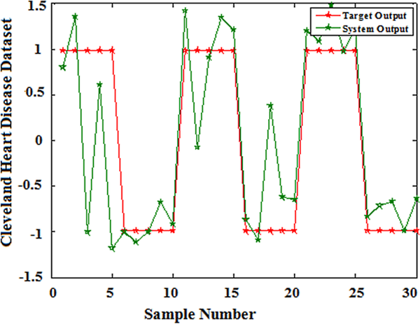
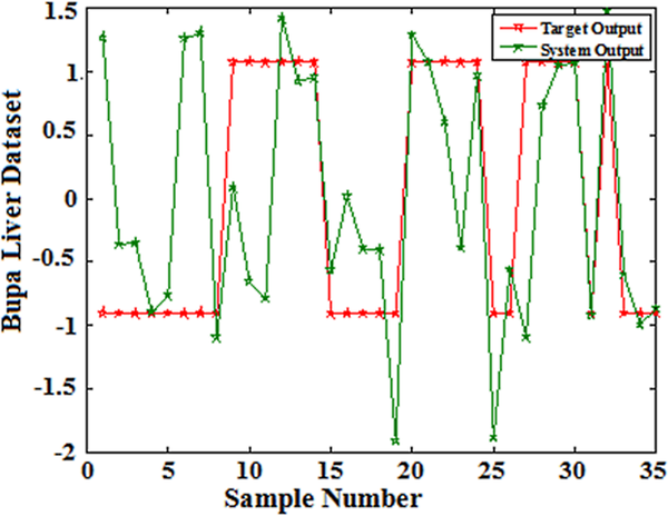
The classification accuracy of the proposed model has been evaluated using 10-fold cross validation of training and testing samples. Figure 2-6 shows the predicted curve for five clinical datasets from the QPSONN model.
| Figure 2. QPSONN prediction curve for hepatitis dataset |
|---|
 |
| Figure 3. QPSONN prediction curve for Wisconsin breast cancer dataset |
|---|
 |
| Figure 4. QPSONN prediction curve for Cleveland heart disease dataset |
|---|
 |
| Figure 5. QPSONN prediction curve for Pima Indian diabetes dataset |
|---|
 |
| Figure 6. QPSONN prediction curve for bupa liver dataset |
|---|
 |
The True Positive (TP), True Negative (TN), False Positive (FP) and False Negative (FN) values are obtained for all the datasets which is represented in Table 5. The TP is the diseased sample correctly diagnosed as a disease. The FP is the normal sample incorrectly identified as a disease. The TN is a normal sample correctly identified as normal. The FN is a diseased sample incorrectly identified as normal.The diagnostic test evaluation has been performed using (MedCalc, 2015) and 95% Confidence Interval (CI) was obtained. CI is a measure of the reliability of an estimate. The measures are computed as follows:
 (16)
(16)
 (17)
(17)
 (18)
(18)
Positive Likelihood Ratio(PLR) (19)
(19)
Negative Likelihood Ratio(NLR) (20)
(20)
Positive Predictive Value(PPV)=  (21)
(21)
Negative Predictive Value(NPV)=  (22)
(22)
Misclassification Rate(MR) (23)
(23)
The PPV and NPV are the probabilities of samples having the disease and samples not having a disease. The NPV and PPV are indirectly proportional to each other. The likelihood ratio is the ratio of the diseased samples to the samples without a disease. The MR gives the proportion of the total number of incorrect predictions. The PLR and NLR are tested for clinical dataset using the QPSONN classifier model and is shown in Table 5.
Table 5. Diagnostic test evaluation for clinical test set
| Performance Measures | PID | WBC | CHD | ||||||
|---|---|---|---|---|---|---|---|---|---|
| 95% Confidence Interval | 95% Confidence Interval | 95% Confidence Interval | |||||||
| From | To | From | To | From | To | ||||
| Sensitivity (%) | 72.22 | 46.52 | 90.31 | 95.45 | 77.16 | 99.88 | 94.44 | 72.71 | 99.86 |
| Specificity (%) | 90.62 | 74.98 | 98.02 | 100 | 95.55 | 100 | 81.48 | 61.92 | 93.70 |
| PLR | 7.70 | 2.53 | 23.49 | - | - | - | 5.10 | 2.29 | 11.34 |
| NLR | 0.31 | 0.14 | 0.65 | 0.05 | 0.01 | 0.31 | 0.07 | 0.01 | 0.46 |
| Disease Prevalence (%) | 36.00 | 22.92 | 50.81 | 21.36 | 13.90 | 30.53 | 40.00 | 25.70 | 55.67 |
| PPV (%) | 81.25 | 54.35 | 95.95 | 100 | 83.89 | 100 | 77.27 | 54.63 | 92.18 |
| NPV (%) | 85.29 | 68.94 | 95.05 | 98.78 | 93.39 | 99.97 | 95.65 | 78.05 | 99.89 |
| MR | 16 | 13.79 | 33.05 | 0.97 | 0.76 | 1.56 | 13.33 | 6.98 | 20.56 |
| Hepatitis | Bupa Liver | ||||||||
| From | To | From | To | ||||||
| Sensitivity (%) | 100 | 54.07 | 100 | 78.57 | 59.05 | 91.70 | |||
| Specificity (%) | 81.25 | 54.35 | 95.95 | 78.26 | 56.30 | 92.54 | |||
| PLR | 5.33 | 1.92 | 14.79 | 3.61 | 1.63 | 8.04 | |||
| NLR | 0.00 | - | - | 0.27 | 0.13 | 0.57 | |||
| Disease Prevalence (%) | 27.27 | 10.73 | 50.22 | 54.90 | 40.34 | 68.87 | |||
| PPV (%) | 66.67 | 29.93 | 92.51 | 81.48 | 61.92 | 93.70 | |||
| NPV (%) | 100 | 75.29 | 100 | 75 | 53.29 | 90.23 | |||
| MR | 13.63 | 6.58 | 21.85 | 21.15 | 15.32 | 37.32 | |||
The diagnostic performance measures used in the classification of datasets are accuracy, sensitivity and specificity. Accuracy measures the performance of the classifier to obtain an accurate diagnosis of the problem set. Sensitivity measures the ability of the model to identify how well the classifier correctly predicts positive samples. Specificity evaluates how well the classifier correctly predicts the negative samples. Comparison of the accuracy of the QPSONN framework and different methods in the literature of all clinical dataset is shown in Table 6.
Table 6. Accuracy comparison of the QPSONN classifier and some existing methods in literature for all clinical test sets
| Author | Method | Accuracy | ||||
|---|---|---|---|---|---|---|
| WBC | PID | CHD | Hepatitis | Bupa Liver | ||
| Proposed | QPSONN | 99.02 | 84 | 86.66 | 86.36 | 76.92 |
| Qasem et al., 2013 | MGANf1f2 | 97.66 | 77.34 | 85.20 | 85.79 | 68.48 |
| MGANf1f3 | 96.78 | 72.78 | 79.07 | 80.04 | 62.63 | |
| MPSONf1f2 | 97.81 | 78.25 | 85.54 | 85.79 | 74.26 | |
| MPSONf1f3 | 97.80 | 68.35 | 80.79 | 79.38 | 63.50 | |
| Abbass, 2001 | MPANN | 98.10 | 74.90 | - | - | - |
| Goh et al., 2008 | HMOENL2 | 96.26 | 78.48 | 79.69 | 80.30 | 68.00 |
| HMOENHN | 96.82 | 75.36 | 81.06 | 75.51 | 68.94 | |
| Cai et al., 2010 | MSCC | 97.60 | 76.50 | - | - | 68.20 |
| Caballero, Martínez, Hervás, & Gutiérrez, 2010 | MPENSGA2E | 95.87 | 78.99 | - | - | - |
| MPENSGA2S | 95.60 | 76.96 | - | - | - | |
| Qasem & Shamsuddin, 2011 | RBFN-TVMOPSO | 96.53 | 78.02 | - | 82.26 | - |
| Antonie et al., 2006 | C4.5 | 93.81 | 76.52 | 76.92 | 83.13 | 71.85 |
| Leung et al., 2012 | RBF network | 95.71 | 74.35 | 84.62 | 84.78 | 62.14 |
| PNN | 95.12 | 70.16 | 73.58 | - | - | |
| KmeansRBF | 96.32 | 74.20 | 81.81 | - | - | |
| KNN | 96.76 | 73.39 | 81.52 | - | - | |
| MLP | 95.44 | 74.76 | 79.22 | - | - | |
| MOA-RBFNN | 95.78 | 79.66 | 86.79 | - | - | |
| Random Forest | 96.19 | 72.61 | 82.42 | 82.58 | 64.08 | |
| SVM | 96.49 | 65.10 | 54.88 | 79.36 | 59.42 | |
| Mangat & Vig, 2014 | CBA | - | 73.45 | 53.85 | 49.50 | 60.90 |
| C Ant Miner PB | - | 74.81 | 55.50 | 72.34 | 66.72 | |
| CMAR | - | 63.94 | 54.45 | 83.33 | 58.14 | |
| ACO/PSO | - | 73.95 | 54.45 | 75.50 | 65.45 | |
| PART | - | 71.73 | 53.83 | 80.15 | 62.70 | |
| DPAC | - | 74.11 | 56.50 | 84.33 | 61.86 | |
| Bhardwaj & Tiwari, 2015 | GONN | 99.63 | - | - | - | - |
A framework for classifying clinical datasets using QPSONN has been proposed in this work. Training the RBFNN has been carried out in two phases. In the first phase, the k-means clustering algorithm has been used to find the optimal number of clusters based on the cluster error. The optimal K clusters serve as hidden nodes in the hidden layer and the cluster centers are used to find the output of the hidden nodes. The second phase of the training is performed between the hidden layer and the output layer based on the MSE using the QPSO algorithm. The accuracy obtained from the QPSONN classifier model is 84% for Pima Indian Diabetes (PID), 86.36% for Hepatitis, 76.92% for Bupa Liver Disease, 99.02% for Wisconsin Breast Cancer (WBC) and 86.66% for Cleveland Heart Disease (CHD) datasets. The classification results show that the QPSONN classifier can be used in clinical decision support system for diagnosing a disease.
This research was previously published in the International Journal of Operations Research and Information Systems (IJORIS), 9(2); edited by John Wang; pages 32-52, copyright year 2018 by IGI Publishing (an imprint of IGI Global).
Abbass, H. A. (2001). A memetic pareto evolutionary approach to artificial neural networks. In Proceedings of the Australian Joint Conference on Artificial Intelligence, Springer Berlin Heidelberg. 10.1007/3-540-45656-2_1
AntonieM. L.ZaianeO. R.HolteR. C. (2006). Learning to use a learned model: A two-stage approach to classification. In Proceedings of the Sixth IEEE International Conference on Data Mining, ICDM’06 (pp. 33-42). 10.1109/ICDM.2006.97
BarretoA. M.BarbosaH. J.EbeckenN. F. (2002). Growing compact RBF networks using a genetic algorithm. In Proceedings of the VII Brazilian Symposium on Neural Networks (pp. 61-66). 10.1109/SBRN.2002.1181436
Bhardwaj, A., & Tiwari, A. (2015). Breast cancer diagnosis using genetically optimized neural network model. Expert Systems with Applications , 42(10), 4611–4620. doi:10.1016/j.eswa.2015.01.065
Blake, C. L., & Merz, C. J. (1998). UCI repository of machine learning databases. Department of Information and computer science, CA: University of California, Irvine. Retrieved December 10, 2014, from http://www.ics.uci.edu/~mlearn/MLRepository
Broomhead, D. S., & Lowe, D. (1988). Radial basis functions, multi-variable functional interpolation and adaptive networks (No. Rsre-Memo-4148) . United Kingdom: Royal Signals and Radar Establishment Malvern.
Caballero, J. C. F., Martínez, F. J., Hervás, C., & Gutiérrez, P. A. (2010). Sensitivity versus accuracy in multiclass problems using memetic pareto evolutionary neural networks. IEEE Transactions on Neural Networks , 21(5), 750–770. doi:10.1109/TNN.2010.2041468
Cai, W., Chen, S., & Zhang, D. (2010). A multiobjective simultaneous learning framework for clustering and classification. IEEE Transactions on Neural Networks , 21(2), 185–200. doi:10.1109/TNN.2009.2034741
Clerc, M., & Kennedy, J. (2002). The particle swarm-explosion, stability, and convergence in a multidimensional complex space. IEEE Transactions on Evolutionary Computation , 6(1), 58–73. doi:10.1109/4235.985692
Dasarathy, B. V., & Sheela, B. V. (1979). A composite classifier system design: Concepts and methodology. Proceedings of the IEEE , 67(5), 708–713. doi:10.1109/PROC.1979.11321
De Castro, L. N. (2006). Fundamentals of natural computing: basic concepts, algorithms, and applications . CRC Press.
De Castro, L. N., & Von Zuben, F. J. (2001). An immunological approach to initialize centers of radial basis function neural networks. In Proceedings of CBRN’01, Brazilian Conference on Neural Networks (pp. 79-84).
Devaraj, D., Yegnanarayana, B., & Ramar, K. (2002). Radial basis function networks for fast contingency ranking. International Journal of Electrical Power & Energy Systems , 24(5), 387–393. doi:10.1016/S0142-0615(01)00041-2
Du, J. X., & Zhai, C. M. (2008). A hybrid learning algorithm combined with generalized rls approach for radial basis function neural networks. Applied Mathematics and Computation , 205(2), 908–915. doi:10.1016/j.amc.2008.05.075
Farzi, S. (2012). Training of fuzzy neural networks via quantum-behaved particle swarm optimization and rival penalized competitive learning. The International Arab Journal of Information Technology , 9(4), 306–313.
Fu, X., & Wang, L. (2003). Data dimensionality reduction with application to simplifying RBF network structure and improving classification performance. IEEE Transactions on Systems, Man, and Cybernetics. Part B, Cybernetics , 33(3), 399–409. doi:10.1109/TSMCB.2003.810911
Goh, C. K., Teoh, E. J., & Tan, K. C. (2008). Hybrid multiobjective evolutionary design for artificial neural networks. IEEE Transactions on Neural Networks , 19(9), 1531–1548. doi:10.1109/TNN.2008.2000444
Han, J., & Kamber, M. (2000). Data mining: concepts and techniques. Morgan Kaufmann.
Han, M., & Xi, J. (2004). Efficient clustering of radial basis perceptron neural network for pattern recognition. Pattern Recognition , 37(10), 2059–2067. doi:10.1016/j.patcog.2004.02.014
Hansen, L. K., & Salamon, P. (1990). Neural network ensembles. IEEE Transactions on Pattern Analysis and Machine Intelligence , 12(10), 993–1001. doi:10.1109/34.58871
Hartigan, J. A., & Wong, M. A. (1979). Algorithm AS 136: A k-means clustering algorithm. Journal of the Royal Statistical Society. Series C, Applied Statistics , 28(1), 100–108.
Hien, D. T. T., Huan, H. X., & Hoang, L. X. M. (2015). An effective solution to regression problem by RBF neuron network. International Journal of Operations Research and Information Systems , 6(4), 57–74. doi:10.4018/IJORIS.2015100104
Karayiannis, N. B. (1997). Gradient descent learning of radial basis neural networks. In Proceedings of the IEEE International Conference on Neural Networks (Vol. 3, pp. 1815-1820). 10.1109/ICNN.1997.614174
Karayiannis, N. B. (1999). Reformulated radial basis neural networks trained by gradient descent. IEEE Transactions on Neural Networks , 10(3), 657–671. doi:10.1109/72.761725
Kurban, T., & Beşdok, E. (2009). A comparison of RBF neural network training algorithms for inertial sensor based terrain classification. Sensors (Basel) , 9(8), 6312–6329. doi:10.3390/s90806312
Leema, N., Nehemiah, H. K., & Kannan, A. (2016). Neural network classifier optimization using Differential Evolution with Global Information and Back Propagation algorithm for clinical datasets. Applied Soft Computing , 49, 834–844. doi:10.1016/j.asoc.2016.08.001
Leonard, J. A., & Kramer, M. A. (1991). Radial basis function networks for classifying process faults. IEEE Control Systems , 11(3), 31–38. doi:10.1109/37.75576
Leung, S. Y. S., Tang, Y., & Wong, W. K. (2012). A hybrid particle swarm optimization and its application in neural networks . Expert Systems with Applications , 39(1), 395–405. doi:10.1016/j.eswa.2011.07.028
Liu, Y., Zheng, Q., Shi, Z., & Chen, J. (2004). Training radial basis function networks with particle swarms. In Proceedings of the International Symposium on Neural Networks (pp. 317-322). Springer Berlin Heidelberg. 10.1007/978-3-540-28647-9_54
MacQueenJ. (1967). Some methods for classification and analysis of multivariate observations. In Proceedings of the fifth Berkeley symposium on mathematical statistics and probability (pp. 281-297).
Mangat, V., & Vig, R. (2014). Dynamic PSO-based associative classifier for medical datasets. IETE Technical Review , 31(4), 258–265. doi:10.1080/02564602.2014.942237
MedCalc. (n.d.). Diagnostic test evaluation calculator, Retrieved March 4, 2015, from https://www.medcalc.org/calc/diagnostic_test.php
Mokeddem, S., & Atmani, B. (2016). Assessment of Clinical Decision Support Systems for Predicting Coronary Heart Disease. International Journal of Operations Research and Information Systems , 7(3), 57–73. doi:10.4018/IJORIS.2016070104
Neelamegam, S., & Ramaraj, E. (2013). Classification algorithm in data mining: An overview. International Journal of P2P Network Trends and Technology, 4 (8), 369-374.
Orr, M. J. L. (1996). Introduction to radial basis neural networks. Center for Cognitive Science, Edinburgh University, Scotland, UK. Retrieved from http://anc.ed.ac.uk/RBNN
Oyang, Y. J., Hwang, S. C., Ou, Y. Y., Chen, C. Y., & Chen, Z. W. (2005). Data classification with radial basis function networks based on a novel kernel density estimation algorithm. IEEE Transactions on Neural Networks , 16(1), 225–236. doi:10.1109/TNN.2004.836229
Qasem, S. N., & Shamsuddin, S. M. (2011). Radial basis function network based on time variant multi-objective particle swarm optimization for medical diseases diagnosis. Applied Soft Computing , 11(1), 1427–1438. doi:10.1016/j.asoc.2010.04.014
Qasem, S. N., Shamsuddin, S. M., Hashim, S. Z. M., Darus, M., & Al-Shammari, E. (2013). Memetic multiobjective particle swarm optimization-based radial basis function network for classification problems. Information Sciences , 239, 165–190. doi:10.1016/j.ins.2013.03.021
Roobaert, D., Karakoulas, G., & Chawla, N. V. (2006). Information gain, correlation and support vector machines . In Feature extraction (pp. 463–470). Springer Berlin Heidelberg. doi:10.1007/978-3-540-35488-8_23
Sadoughi, F., Ghaderzadeh, M., Fein, R., & Standring, A. (2014). Comparison of back propagation neural network and back propagation neural network based particle swarm intelligence in diagnostic breast cancer. Applied Medical Informatics , 34(1), 22.
Simon, D. (2002). Training radial basis neural networks with the extended Kalman filter. Neurocomputing , 48(1), 455–475. doi:10.1016/S0925-2312(01)00611-7
Sun, J., Fang, W., Palade, V., Wu, X., & Xu, W. (2011). Quantum-behaved particle swarm optimization with Gaussian distributed local attractor point. Applied Mathematics and Computation , 218(7), 3763–3775. doi:10.1016/j.amc.2011.09.021
Sun, J., Fang, W., Wu, X., Palade, V., & Xu, W. (2012). Quantum-behaved particle swarm optimization: Analysis of individual particle behavior and parameter selection. Evolutionary Computation , 20(3), 349–393. doi:10.1162/EVCO_a_00049
SunJ.FengB.XuW. (2004a). Particle swarm optimization with particles having quantum behavior. In Proceedings of the IEEE Congress on Evolutionary Computation, CEC2004 (pp. 325-331). 10.1109/CEC.2004.1330875
SunJ.XuW.FengB. (2004b). A global search strategy of quantum-behaved particle swarm optimization. In Proceedings of the IEEE Conference on Cybernetics and Intelligent Systems (pp. 111-116).
Sun, J., Xu, W., & Feng, B. (2005). Adaptive parameter control for quantum-behaved particle swarm optimization on individual level. In Proceedings of the IEEE International Conference on Systems, Man and Cybernetics (Vol. 4, pp. 3049-3054). 10.1109/ICSMC.2005.1571614
Susmi, S. J., Nehemiah, H. K., Kannan, A., & Christopher, J. J. (2015). A hybrid classifier for leukemia gene expression data. Research Journal of Applied Sciences, Engineering and Technology , 10(2), 197–205.
Tarassenko, I., & Roberts, S. (1994). Supervised and unsupervised learning in radial basis function classifiers. IEE Proceedings. Vision Image and Signal Processing , 141(4), 210–216. doi:10.1049/ip-vis:19941324
Tryon, R. C. (1939). Cluster analysis: Correlation profile and orthometric (factor) analysis for the isolation of unities in mind and personality. Edwards brother, Incorporated, lithoprinters and publishers.
Wang, L., Chen, K., & Ong, Y. S. (2005). Advances in natural computation: Pt. 1. In Proceedings of the First International Conference, ICNC 2005, Changsha, China, August 27-29. Springer Science & Business Media.
Xu, L., Krzyzak, A., & Oja, E. (1993). Rival penalized competitive learning for clustering analysis, RBF net, and curve detection. IEEE Transactions on Neural Networks , 4(4), 636–649. doi:10.1109/72.238318
YuB.HeX. (2006). Training radial basis function networks with differential evolution. In Proceedings of IEEE International Conference on Granular Computing.