1 Introduction
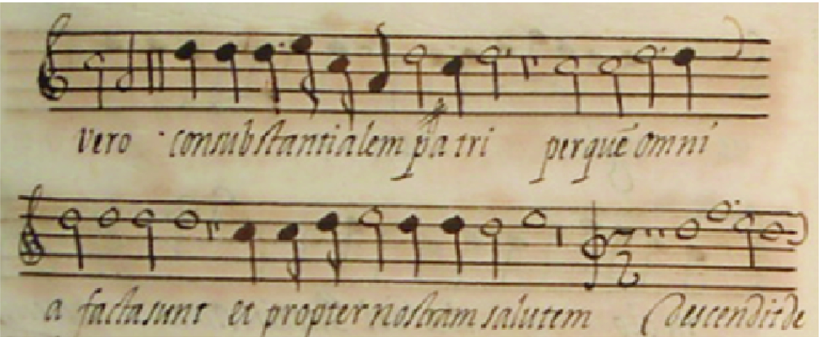
The kind of documents processed (here a fragment of a page) are single-voice vocal music written in the Spanish variant of the white mensural notation.
The automatic pattern recognition approach has been traditionally focused on accomplishing a fully-automated operation. Nevertheless, in our approach, complete automation is not possible, although a perfect transcription of the original documents is needed for editing and publishing a collection. Therefore, we have to focus on the human-machine interaction tasks and how to optimize the expert user feedback loop [6].
The errors made by the system are usually seen as an issue outside the research process because correcting them is considered as the procedure for converting the system hypothesis into the desired result. However, semi-automatic approaches in which the human operator has the eventual responsibility of verifying and completing the task are the key to an efficient solution [7].
In this paper, we will study how using the user’s corrections help the classifier to learn its model incrementally, decreasing the error throughout the task. Deep convolutional neural nets (DCNN) [3] are improving the state of the art in computer image analysis tasks. Although there are works already that permit to modify these recognition models as a continuous learning process as new classes of data arrive [9], the task is still computationally demanding. We explore the possibility of combining the ability of DCNN for extracting good image features, with the simplicity of a nearest-neighbor (1-NN) classifier to adapt its performance to a specific training set along the edition stage.
2 Data Structure
 annotated with their ground-truth categories. This way, each page
  can be considered as a training subset
  , where the
  represent the symbol bounding boxes in page
  and
and  their corresponding labels.
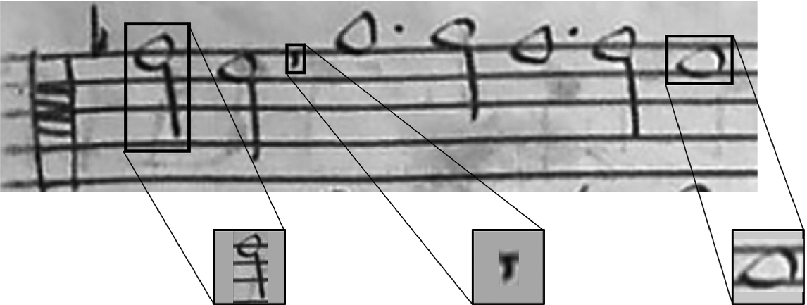
Examples of bounding boxes for some symbols and how they are adapted to a  window in different situations. (Left and right:) fit to a
  window, keeping aspect ratio and background padding; (center:) no bounding box stretching is done when it is smaller than the target window.
The symbol bounding boxes were extracted from the image and re-scaled to a  -pixel window (only if the bounding box is bigger than that), keeping the aspect ratio of the box and padding the background with its maximum pixel value (see Fig. 2 for some examples).
When this window is the input for the DCNN, no additional processing is made, since the filters of the network input layer process the window regardless of its size. Nevertheless, the 1-NN will classify every window considering it as a vector ![$$\mathbf{x} \in [0,255]^{30\times 30}$$](../images/496776_1_En_40_Chapter/496776_1_En_40_Chapter_TeX_IEq10.png) . Due to its sensitivity to the dimensionality of the feature space, we have transformed the windows by downsampling, keeping the central pixel of every non-overlapping
. Due to its sensitivity to the dimensionality of the feature space, we have transformed the windows by downsampling, keeping the central pixel of every non-overlapping  pixel area, assigning to it the mean of the 9 pixels involved. This is equivalent to low-pass filtering of the window, keeping the main features of the image in a smaller space (
![$$[0,255]^{10\times 10}$$](../images/496776_1_En_40_Chapter/496776_1_En_40_Chapter_TeX_IEq12.png) ).
).
3 Incremental Learning
The key point in this work is to study how can we adapt the recognition model to the data and do it incrementally. In real operation, a collection of scores is presented to the user by pages. Each page is processed, and the symbols are classified (see [1] for details). Then, the user makes corrections to the symbols that were incorrectly classified. This happens when the system hypothesis does not match the ground-truth label or when the symbol belongs to previously unseen classes. User corrections will be simulated. These interactions are utilized to improve the model for the classification of the next pages.
The recognition algorithm (the model  ) is a key issue in any pattern classification system, but in an interactive architecture, the most relevant feature is the ability of the algorithm to adapt to the specificities of the data through the error corrections made by the user. In the interactive paradigm, the efficient exploitation of human expert knowledge is the main objective, so the correctness of the system output is no longer the main issue to assess. The challenge now is the development of interactive schemes capable of efficiently exploiting the feedback to eventually reduce the user’s workload.
In light of that, we have selected a very simple, but flexible, classification algorithm as the nearest neighbor is. It does not need a parametric analysis of the feature space for operation, and the training set  can be incrementally built by adding new pairs as they are found in the input in operation time:
  . Only an initial model
  , trained offline, is needed to start classifying. This model can be trained with the symbols on the first page
  , including the labels for the symbols on it,
  , or with an initial subset of pages if the model needs more examples, as explained below.
Also, it is easy to add new classes dynamically by adding new labels, if needed. Besides, editing and condensing methods [8] can be easily applied to the training set if advised by the user corrections. The system must operate in real-time, so the user can interact with it comfortably. This is another feature that advises using simple, adaptive, and fast classification algorithms.
 can be due to symbols belonging to unseen classes. In such a case, the interaction step includes the addition of the new class to the training set, with the symbols seen on the current page as prototypes. This algorithm will try to minimize the number of errors
  , and so the need of user corrections, as the pages are processed.
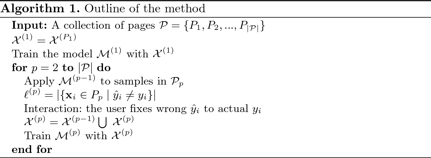
This algorithm does not change independently of the classification model utilized,  . Only the
  considered might be different, as explained below.
We want to explore a trade-off between accuracy in the classification and speed and flexibility in re-training the model. DCNN are state-of-the-art image classification methods, but the usual size of these models make their adaptation difficult and time-consuming. On the other hand, in many classical classification algorithms, like the 1-NN, the adaptation is straightforward, because it needs only updating the training set to adapt to a new situation in real-time (we consider as real-time any situation in which the user does not perceive that he or she has to wait for the system to make a decision).
- 1.
DCNN: the model
 is a deep convolutional neural network. It is expected to achieve good performance (low error rates) but long retraining times.
 - 2.
1-NN:
 is a nearest neighbor classifier. Retraining and recognition can be done in real time, but higher error rates are expected.
 - 3.
NC+1NN: A DCNN learned on a subset of initial pages of
 is used as a feature extractor (neural codes [2], NC) and the 1-NN is applied to the NC to implement the incremental classification described in the algorithm.
 filters each. Then, a global max-pooling layer provides a
  vector that will be the NC features for the nearest neighbor (in the case 3.) or fully connected to a layer with as many neurons as classes that will be classified with a softmax in the case of full DCNN classification (1.). The network architecture is displayed in Fig. 3. For training, Adam optimization has been used with a learning rate of 0.001 during 100 epochs, using minibatches of 64 images. Units have ReLU activations.
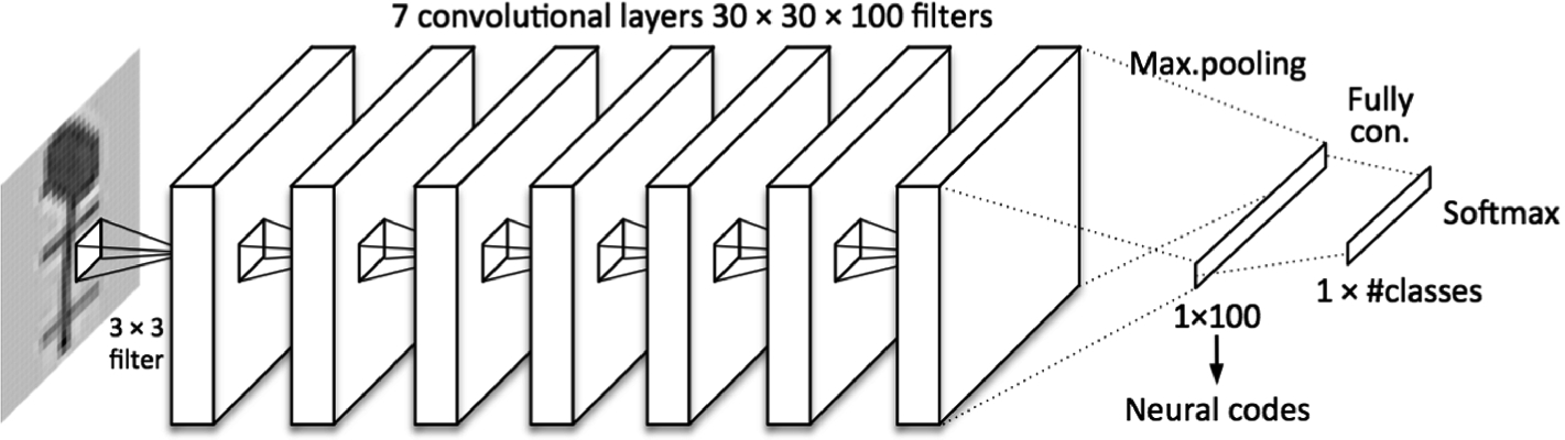
Architecture of the DCNN used. Neural codes are the activations of the 100-neuron layer after pooling. For that, the last layer is removed and the neuron activations are the input to a nearest neighbor classifier.
4 Data and Results
We have selected a Mass in A minor from a collection of sacred vocal music from the 17th century. In this case, we have  pages. Each page has a maximum of 6 staves of monophonic music, containing between 20 and 30 symbols each on average, for a total of 17,114 samples.
Initial Training Set. According to the instructions in Algorithm 1, the initial training set is  , but some considerations about this follow.
The number of prototypes in  is 143 from 23 classes. The C and F clefs received special consideration. Since the initial pages were written in the G clef, 6 prototypes of each of the other clefs were included in
  from other composition. This way,
  prototypes from 25 classes.
When the DCNN is utilized, either as a classifier or for feature extraction, we need more data to train such a large structure properly. For that, an initial subset of the first 16 pages was considered:  . This way,
  2440 + 12 prototypes from 44 classes. In this case, the Algorithm 1 runs for
  to
to  .
.
As the algorithm runs, the number of classes will increase. Each time an unseen class appears, it produces errors. As this page is included in the training set for the next step, the unknown class appears for the next iteration. The final number of classes is 53 for this composition.
Results. First, a study of the difference between with and without interaction is shown (see Fig. 4). The graph shows that, when the user corrections are used, a rapid drop in the error rate for the 1-NN is initially observed. The error rises again when another voice of the same composition begins to be processed. When the effect of the new pages is learned by the model, it is able to reduce the error again. Every time a change in the conditions happens the system degrades its performance, but it is able to continue learning later on, improving its performance.
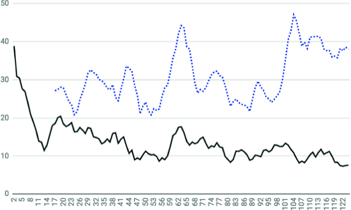
Smoothed evolutions of the error rate (%) along the 124 pages of the studied composition, using 1-NN for classification. In solid line: error rate when using the interactive scheme. In dotted line: error rate without interaction, using a fixed training set.
One interesting feature is that pages from 60 to 65 have specificities not seen before. In that situation, both curves degrade. But when a similar situation occurs again from page 100 onwards, the incremental method is robust against that particular situation (solid line), while the non-incremental method is not and its performance degrades again.
 , but when the nets are used they use the first 16 pages for initial training, so the results are displayed from
  .
.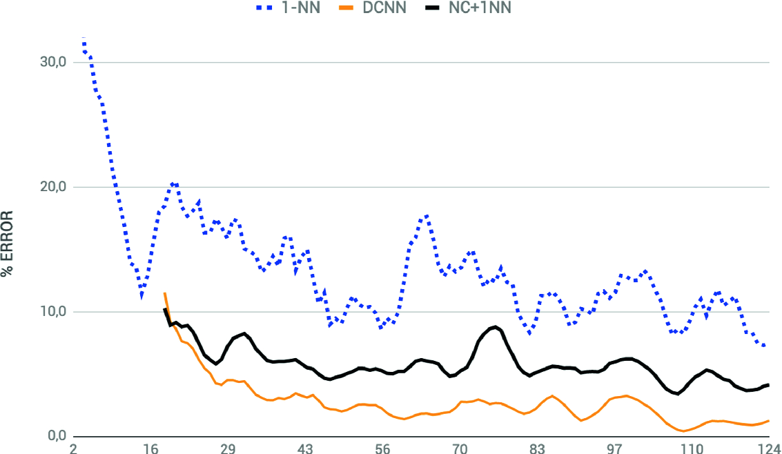
Evolution of the error rates for the different methods considered. 1-NN (dotted): only nearest neighbors classifying the pixel values; DCNN (thin solid): only deep convolutional nets classifying the bounding boxes; NC + 1NN (thick solid): nearest neighbors classifying the extracted neural codes.
The 1-NN adapts the best but performs the worst (an average error of 9.6% for the last 15 pages), but it runs in real time, without the user noticing any delay. On the other hand, the DCNN is able to reach a 1.1% of error at the end, but running the whole Algorithm 1 using that model took 7749 s in a GPU computer (note from Algorithm 1 that the network is retrained with the new training set after each page). The 1-NN applied to the neural codes was able to adapt to the data (less than using the 1-NN alone), reaching a nice 4.4% of error at the end. This approach works in real time, since the network learning is made only once, before starting the classification and adaptation.
5 Conclusion
The presence of the expert user in the learning loop opens up new possibilities for study adaptive learning algorithms. The presented study shows that a combination of DCNN acting as a feature extractor and a nearest neighbor for classifying the extracted neural codes can provide a good trade off between precision and real-time operation. In any case, there are many ways left to be explored to make the human-in-the-loop approach efficient and effective.
Work supported by the Spanish Ministry HISPAMUS project TIN2017-86576-R, partially funded by the EU.