III.84 The Simplex Algorithm
Richard Weber
1 Linear Programming
The simplex algorithm is the preeminent tool for solving some of the most important mathematical problems arising in business, science, and technology. In these problems, which are called linear programs, we are to maximize (or minimize) a linear function subject to linear constraints. An example is the diet problem posed by the U.S. Air Force in 1947: find quantities of seventy-seven differently priced foodstuffs (cheese, spinach, etc.) to satisfy a man’s minimum daily requirements for nine nutrients (protein, iron, etc.) at least cost. Further applications occur in choosing the elements of an investment portfolio, rostering an airline’s crew, and finding optimal strategies in two-person games. The study of linear programming has inspired many of the central ideas of optimization theory, such as DUALITY [III.19], the importance of convexity, and COMPUTATIONAL COMPLEXITY [IV.20].
The input data of a linear program (LP) consists of two vectors b ∈  m and c ∈
  n, and an m × n matrix A = (aij). The problem is to find values for n non-negative decision variables, x1, . . . , xn, to maximize the objective function c1x1 + . . . + cnxn, subject to m constraints, ai1x1 + . . . + ainxn ≤ bi, i = 1, . . . , m. In the diet problem, n = 77 and m = 9. In the following simple example (not a diet problem), n = 2 and m = 3. In serious real-life problems, n and m can be greater than 100 000.
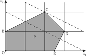
Figure 1 Feasible region “P” of an LP.
Maximize x1 + 2x2
subject to -x1 + 2x2 ≤ 2,
x1 + x2 ≤ 4,
2x1 - x2 ≤ 5,
x1, x2 ≥ 0.
The constraints define a feasible region for (x1, x2), a convex polygon that is depicted by the shaded region “P” in figure 1. The two dotted lines mark those x where the value of the objective function value is 4 and where it is 6. Clearly, it is maximized at point C.
The general story is similar to that of the example. If the feasible region P = {x : Ax ≤ b, x ≥ 0} is nonempty, then it is a convex polytope in Rn, and an optimal solution can be found at one of its vertices. It is helpful to introduce “slack variables” x3, x4, x5 ≥ to take up the slack on the left of the inequality constraints. We can write

We now have three equations in five variables, so we can set any two of the variables x1, . . . , x5 equal to 0, and solve the equations for the other three variables (or solve a perturbation of them if they happen not to be independent). There are ten ways to choose two variables from five. Not all of the ten corresponding solutions satisfy x1, x2, x3, x4, x5 ≥ 0, but five of them do. These are called basic feasible solutions (BFSs), and correspond to the vertices of P marked O, B, C, D, E.
2 How the Algorithm Works
George Dantzig invented the simplex algorithm in 1947 as a means of solving the Air Force’s diet problem mentioned at the start. The word “program” was not yet used to mean computer code, but was a military term for a logistic plan or schedule. The fundamental fact on which the algorithm relies is that if an LP has a bounded optimal solution, then the optimum value is attained at a BFS, i.e., at a vertex (or so-called “extreme point”) of the polytope of feasible points, P. Another name for the feasible polytope is “simplex,” which is where the algorithm gets its name. It works as follows.
Step 0. Pick a BFS.
Step 1. Test whether this BFS is optimal. If so, stop. If not, go to step 2.
Step 2. Find a better BFS.
Repeat from step 1.
Since there are only finitely many BFSs (i.e., vertices of P), the algorithm must stop.
Now that we have an overview, let us look at the details. Suppose that at step 0 we pick the BFS of x = (x1, x2, x3, x4, x5) = (0, 0, 2, 4, 5), corresponding to vertex O. At step 1 we wish to know whether the objective function can be increased if x1 or x2 is increased from 0. So we write x3, x4, x5, and the objective function cTx in terms of x1 and x2, and display this as dictionary 1.
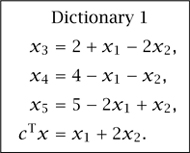
The last equation in the dictionary shows that we can increase the value of cTx by increasing either x1 or x2 from 0. Suppose that we increase x2. The first and second equations show that x3 and x4 must decrease, and we cannot increase x2 beyond 1, at which point x3 = 0 and x4 = 3, x5 = 6. Increasing x2 as much as possible, we complete step 2 and arrive at a new BFS of x = (0, 1, 0, 3, 6), which is vertex B. Now we are ready for step 1 again, and so we write x2, x4, x5, and cTx in terms of the variables that are now zero, namely x1, x3, to give dictionary 2.
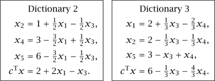
This shows that cTx can be increased by increasing x1 from 0, but that x1 can increase no further than 2 because at that point x4 = 0. This brings us to a new solution (2, 2, 0, 0, 3), which is vertex C. Once more, we are ready for step 1, and so compute dictionary 3, now writing things in terms of x3 and x4, which are 0. The algorithm now stops because, as we require x3, x4 ≥ 0, the bottom line of dictionary 3 proves that cTx ≤ 6 for all feasible x.
There is other important information in the final dictionary. If b is changed to b + ψ, for small ψT = (ψl, ψ2, ψ3), then the maximum value of cTx will change to  . The coefficient
  is called a “shadow price,” because it is what we should be willing to pay per unit increase in b1.
3 How the Algorithm Performs
In running the simplex algorithm the serious work comes in computing the dictionaries. To find dictionary 2, we could use the first equation of dictionary 1 to rewrite x2 in terms of x1 and x3, and then substitute for x2 in the other equations. Versions of the simplex algorithm have been invented that reduce the computing effort by taking advantage of special structure in the matrix A, such as the fact that most of its entries are zero. The dictionary data is often held in a so-called tableau of coefficients.
There are many other practical and theoretical issues. One concerns the selection of the pivot, that is, the variable that is to be increased from 0. Starting at 0, and depending on which of x1 and x2 we choose as the first variable to increase from zero, the path to C can be 0, E, D, C or 0, B, C. There is no known way to guarantee that the algorithm takes the shortest path.
The question of how many steps the simplex algorithm really needs is related to the famous Hirsch conjecture: that for any bounded n-dimensional polytope with m faces, the diameter (defined as the maximum number of edges on the shortest edge-traversing path between any two vertices) is at most m - n. If this were true, it would suggest that some version of the simplex algorithm might run in a number of steps that grows only linearly in the numbers of variables and constraints. However, Klee and Minty (1972) have given an example based on a perturbed n-dimensional cube (m = 2n faces and diameter n), in which if the algorithm selects among possible pivots by choosing the one for which the objective function increases at the greatest rate per unit increase in that variable, then it visits all 2n vertices before reaching the optimum. Indeed, for most deterministic pivot selection rules, examples are known in which the number of steps grows exponentially in n.
Fortunately, things are usually much better in practical problems than in worst-case examples. Typically, only 0(m) steps are needed to solve a problem with m constraints. Moreover, Khachian (1979) proved (by analysis of the so-called ellipsoid algorithm) that linear programs can in principle be solved by an algorithm whose running time grows only polynomially in n. Thus linear programming is much easier than “integer linear programming,” in which x1, . . . , xn are required to be integers and for which no algorithm with polynomial running time is known.
Karmarkar (1984) pioneered development of “interior” methods for linear programming problems. These move through the interior of the polytope P, rather than among its vertices, and can sometimes solve large LPs more quickly than the simplex algorithm. Modern computer software uses both methods and can easily solve LPs with millions of variables and constraints.
Further Reading
Dantzig, G. 1963. Linear Programming and Extensions. Princeton, NJ: Princeton University Press.
Karmarkar, N. 1984. A new polynomial-time algorithm for linear programming. Combinatorica 4:373-95.
Khachían, L. G. 1979. A polynomial algorithm in linear programming. Soviet Mathematics Doklady 20:191-94.
Klee, V., and G. Minty. 1972. How good is the simplex algorithm? In Inequalities III, edited by O. Shisha, volume 16, pp. 159-75. New York: Academic Press.
Solitons
See LINEAR AND NONLINEAR WAVES AND SOLITONS [III.49]
 m and c ∈
  n, and an m × n matrix A = (aij). The problem is to find values for n non-negative decision variables, x1, . . . , xn, to maximize the objective function c1x1 + . . . + cnxn, subject to m constraints, ai1x1 + . . . + ainxn ≤ bi, i = 1, . . . , m. In the diet problem, n = 77 and m = 9. In the following simple example (not a diet problem), n = 2 and m = 3. In serious real-life problems, n and m can be greater than 100 000.


 . The coefficient
  is called a “shadow price,” because it is what we should be willing to pay per unit increase in b1.