15
Control of the Electric Drive

“It has recently come to my attention that my good friend James Clerk Maxwell has had some difficulty with a rather trivial problem …”

Edward John Routh (1831–1907) [1].

In this chapter, basic control theory is applied to the electric vehicle powertrain propelled by the dc machine. The basics of control apply whether the machine is dc or ac, and so the integration of the permanent‐magnet (PM) dc machine is the starting point. The wound‐field (WF) dc machine is then used to enable high‐speed field‐weakened operation of the electric vehicle. MATLAB/Simulink is used to simulate the drive.

15.1 Introduction to Control

Control is one of the key technical areas of electrical power conversion and electric drives, as we are always interested in controlling the voltage, current, frequency, torque, speed, and so on. The application of feedback control has contributed greatly to the industrial age. The first industrial controller was developed by James Watt (1736–1819) to regulate his steam engine. James Clerk Maxwell (1831–1879) is acknowledged as one of the great minds of science and mathematics, and is credited with initially developing control theory. Maxwell and his electromagnetic equations feature prominently in Chapter 16. Edward John Routh (1831–1907), a classmate of Maxwell at the University of Cambridge in England, also made some great contributions to control theory and stability analysis. In a distinguished class at Cambridge, Routh actually finished just above Maxwell in the graduating class of 1854.

Hendrik Bode (1905–1982) and Harry Nyquist (1889–1976) further developed and applied control theory as we learn it today.

From an electric drive perspective, there are two main feedback control loops on a vehicle. The outer loop is the vehicle speed loop. This loop is a relatively slow loop and is generally closed in the brain of the human driver. Obviously, the role of the driver in controlling the vehicle speed is changing with the advent of autonomous self‐driving vehicles. The second main loop is the torque command, which essentially is fed into the vehicle powertrain by stepping on the accelerator or brake. This loop is significantly faster than the speed loop, and the vehicle responds rapidly to regulate the machine torque.

This inner torque loop is essentially a current loop in the electric vehicle. Current is easily regulated and is proportional to the machine torque. The outer loop is the speed loop. As speed is proportional to the voltage, this loop can also be the voltage loop in an industrial controller.

15.1.1 Feedback Controller Design Approach

Controlling and stabilizing a feedback controller can be quite technical and mathematical, but also practical. See references [1–7] for further study.

In this investigation, we will make some simplifying assumptions in order to develop basic controllers.

There are four main steps to closing the feedback loop.

First, large‐signal models are developed to characterize the system.

Second, the large‐signal model is linearized around a dc operating point and investigated using small‐signal analysis.

Third, the system is stabilized by applying feedback control theory to the small‐signal model.

Finally, the system is tested for a dynamic response using the large‐signal models.

In this system, we use two loops as shown in the control block diagram of Figure 15.1. The inner torque/current loop is very fast – typically, this loop has a crossover frequency, also known as the bandwidth, of about 1/10th of the switching frequency, for example, 500 Hz for a 5 kHz switching frequency. The outer loop is the speed loop and is much slower. In a typical industrial application, the bandwidth of the outer loop would be significantly lower than the current loop, perhaps 1/10th or less of the current‐loop bandwidth. When the human driver is the regulator, the speed bandwidth is about 5 Hz, a reasonable estimate for the response time of the driver.

Figure 15.1 Control block diagram.

The outer speed loop is closed in the brain of the driver. The driver can change the speed of the vehicle by requesting more or less torque from the drive system using the accelerator or brake pedal. The speed error is amplified by the speed error amplifier G_cω within the human brain. The output of the speed error amplifier is the input command to the torque/current loop, the input mechanism being the accelerator and brake pedals in the case of the vehicle.

15.2 Modeling the Electromechanical System

In this section, large‐ and small‐signal models are developed for the mechanical system, the permanent‐magnet (PM) dc machine, the dc‐dc converter‚ and the proportional‐integral (PI) controller. The overall system is shown in Figure 15.2.

Figure 15.2 Simulink model of electric vehicle (EV) with PM dc drive.

15.2.1 The Mechanical System

The mechanical system can be modeled using the earlier torque equation, Equation (2.26) from Chapter 2 and letting rotor torque T_r equal traction torque T_t:

The vehicle road‐load force and torque are

(15.1)

The axle and accelerating torques, T_axle and T_a, respectively, are

(15.2)

and

(15.3)

We know that

(15.4)

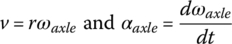
Thus, the accelerating torque is

(15.5)

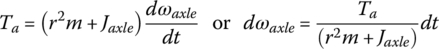
where J_axle is the equivalent moment of inertia (MOI) referenced to the drive axle.

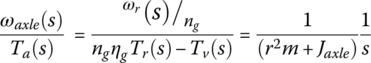
The final part of the equation can be formatted as an integral to give the axle speed ω_axle in rad/s:

(15.6)

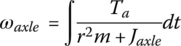
This expression can be written as a Laplace transform:

(15.7)

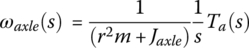
where s is the complex operator.

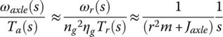
We can substitute in the relationships between rotor speed and torque to axle speed and accelerating torque, respectively, as follows:

(15.8)

The large‐signal model just presented relates speed as an output to torque as an input. The large‐signal mechanical system based on the earlier equations is presented in Figure 15.3.

Figure 15.3 Simulink model of mechanical system.

For a small‐signal perturbation, the effects of the vehicle load and slope forces can be ignored due to the large inertia of the vehicle. In such a case:

(15.9)

This equation can be modified to determine the small‐signal relationship between rotor torque and rotor speed. The equation when modified as follows yields the small‐signal gain of the mechanical system:

(15.10)

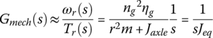
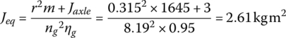
where J_eq is the equivalent small‐signal inertia of the system as seen from the rotor:

(15.11)

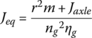
We now have the large‐ and small‐signal models for the mechanical system.

15.2.2 The PM DC Machine

The PM dc machine model is now developed. The basic machine equations from Chapter 7 are as follows:

(15.12)

(15.13)

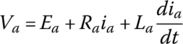
and

(15.14)

The circuit equation is reformatted to integral form:

(15.15)

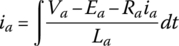
and as a Laplace transform:

(15.16)

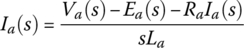
For a small‐signal perturbation, the effects of the back emf E_a (and speed) can be ignored due to vehicle inertia. Thus, the small‐signal gain of the machine is given by

(15.17)

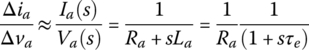
where τ_e, which equals L_a/R_a, is the electrical time constant of the machine.

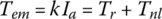
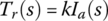
The relationship between the rotor torque and current is

(15.18)

The effect of no‐load torque can be ignored, and the small‐signal relationship between rotor torque and armature current is

(15.19)

Thus, the small‐signal gain of the dc machine G_dcm can be modeled as

(15.20)

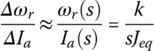
Combining Equation (15.10) and Equation (15.13), the relationship between rotor speed and armature current can be easily derived as

(15.21)

The large‐signal machine equations are built into a Simulink model as shown in Figure 15.4. Note that the machine moment of inertia is ignored as it is negligible compared to the vehicle inertia.

Figure 15.4 Simulink model of dc machine.

15.2.3 The DC‐DC Power Converter

The full‐bridge dc‐dc converter is operated using current‐mode control. The machine torque can be controlled by regulating the armature current.

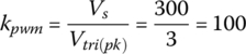
From a control perspective, the dc‐dc converter can be seen as an amplifier with a gain k_pwm given by

(15.22)

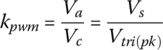
where voltage V_c is the amplifier control voltage, which is amplified by gain k_pwm to provide the amplifier output voltage V_a, and then supplied to the armature terminals of the machine. The gain can be shown to be the ratio of the dc voltage feeding the amplifier V_s to the peak of the triangular voltage V_tri(pk) used for pulse‐width‐modulation (PWM) signal generation.

15.2.4 The PI Controller

A PI controller can be used for controlling both the torque and speed loops.

The PI error amplifier is shown in Figure 15.5, and is simply modeled as

(15.23)

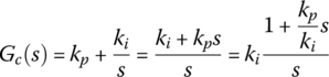
Figure 15.5 PI controller.

The error amplifier has a gain k_i with a pole at 0 Hz or dc, and a zero determined by k_p/k_i.

15.3 Designing Torque Loop Compensation

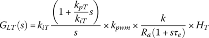
The loop gain of the torque loop G_LT(s) is as follows:

(15.24)

where G_cT(s) and H_T(s) are the gains of the PI error amplifier in the torque loop and of the feedback stage, respectively.

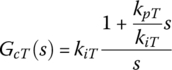
The gain of the torque‐loop PI error amplifier is

(15.25)

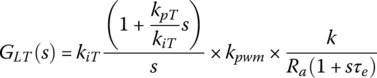
For simplicity, the feedback gain H_T(s) is set to unity. Thus, the torque‐loop gain simplifies to

(15.26)

In greater detail:

(15.27)

For simplicity, the loop can be easily stabilized by placing the compensator zero such that it cancels the pole due to the motor. Thus, let

(15.28)

This simplifies Equation (15.27) to

(15.29)

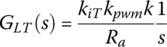
which represents a single pole with a phase of −90°.

Let the bandwidth or crossover frequency of the current‐control loop be ω_cT. The loop gain is unity at the crossover frequency. Thus, once the bandwidth is specified, the compensator parameters are easily determined:

(15.30)

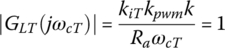
resulting in an expression for the integral gain:

(15.31)

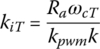
Now Equation (15.28) can be used to determine the proportional gain.

15.3.1 Example: Determining Compensator Gain Coefficients for Torque Loop

The system parameters of a PM dc motor supplied by a current‐controlled switch‐mode PWM dc‐dc converter are as follows: armature resistance R_a = 50 mΩ, armature inductance L_a = 0.5 mH, converter dc bus voltage V_s = 300 V, amplitude of triangular waveform control voltage V_tri(pk) = 3 V, switching frequency f_s = 10 kHz, and machine constant k = 0.77 Nm/A. The motor is controlled by an inner loop controlling torque (current). The feedback effects of the motor‐induced back emf and the load torque on the control loop can be neglected.

Calculate the error amplifier proportional and integral gains k_pT and k_iT in order for the torque loop to have a single‐pole roll‐off characteristic with the crossover frequency at one tenth of the switching frequency, that is, 1000 Hz. Assume unity feedback.

Solution:

The electrical time constant and converter gain are

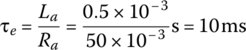
and

Assuming a single‐pole roll‐off, we know from Equation (15.31) that

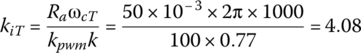
and from Equation (15.28) that

15.4 Designing Speed Control Loop Compensation

The loop gain of the speed loop G_Lω is as follows:

(15.32)

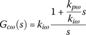
where G_CLT is the closed‐loop gain of the inner torque loop, and H_ω(s) is the speed feedback gain. The gain of the speed‐loop PI error amplifier is

(15.33)

As the speed loop is a much slower loop, we can assume that the torque loop is ideal and that its gain is unity, that is, G_CLT(s)=1. For simplicity, let us also set the feedback gain H_ω(s) to unity.

Thus, the speed‐loop gain can be simplified to

(15.34)

or

(15.35)

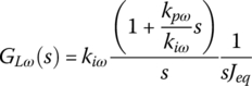
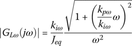
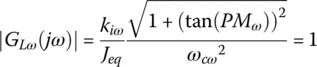
which represents a function with two poles at dc plus a zero at a frequency determined by the controller gains. The magnitude of the loop gain is given by

(15.36)

The phase of the loop is

(15.37)

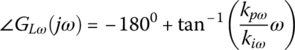
as the two poles at dc provide a phase of −180°. The phase of the zero at the crossover frequency provides the speed‐loop phase margin.

Thus, the phase margin PM_ω of the speed loop is

(15.38)

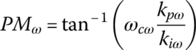
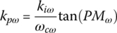
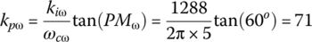
If the desired phase margin is known, then the proportional gain can be determined from

(15.39)

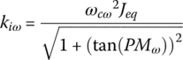
The gain at the crossover frequency is

(15.40)

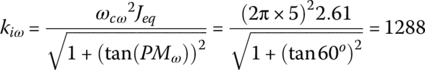
Thus, the integral gain is given by the following equation:

(15.41)

15.4.1 Example: Determining Compensator Gain Coefficients for Speed Loop

The vehicle of the earlier example is controlled by an outer speed loop with a bandwidth of 5 Hz and a phase margin of 60°. Let the mass m = 1645 kg, wheel radius r = 0.315 m, gear ratio n_g = 8.19, gear efficiency η_g= 95%, and the axle‐referenced MOI J_axle = 3 kgm². Assume a feedback of unity for the speed loop.

Calculate the error amplifier proportional and integral gains k_pω and k_iω.

Solution:

The equivalent MOI is

The PI coefficients are

and

The PM dc drive simulation in the next section is controlled using the parameters derived in the two previous examples.

15.5 Acceleration of Battery Electric Vehicle (BEV) using PM DC Machine

A controlled drive acceleration of the vehicle can now be simulated as the control coefficients are known, and can be used in the Simulink model of Figure 15.2. A simple acceleration of the vehicle from 0 to 100 km/h is simulated and plotted in Figure 15.6. The machine armature voltage V_a, armature current I_a and vehicle speed in km/h are shown in Figure 15.6.

Figure 15.6 PM dc drive simulation outputs.

As discussed in Chapter 7, Section 7.1.7, the conventional PM dc machine cannot be field weakened, and so it is not possible to operate it significantly beyond the rated speed of about 39.56 km/h for the example. As the vehicle accelerates, the machine back emf increases from 0 V to 300 V at 50 km/h. As the maximum voltage of 300 V has been reached, the vehicle cannot speed up anymore, and the speed is clamped at about 50 km/h. The armature current drops significantly from the initial high value to enable acceleration to the much lower value required to cruise at about 50 km/h.

15.6 Acceleration of BEV using WF DC Machine

The PM dc machine model of Figure 15.2 is now replaced with a WF dc machine. The WF dc machine model is as shown in Figure 15.7 and Figure 15.8. Note that the control coefficients are not changed in this simple simulation.

Figure 15.7 Simulink model of WF dc drive.

Figure 15.8 Simulink model of WF dc machine.

As discussed in Chapter 7, Section 7.1.8, the field current I_f is reduced proportionately with speed above the rated speed to enable high‐speed operation by field weakening. The machine constant is given by

(15.42)

where the field current is speed dependent as follows:

(15.43)

As the WF dc machine can be field weakened to the maximum speed of 150 km/h, the vehicle can provide full acceleration to 100 km/h, as shown in Figure 15.9. This simple example illustrates the benefits of field‐weakening an electrical machine to enable high‐speed operation.

Figure 15.9 WF dc drive simulation scope outputs.

As shown in Figure 15.9, the vehicle can speed up above the rated speed and can maintain maximum current flow into the machine as the machine speed is not limited by the back emf due to the field weakening.

References

1. 1 J. G. Truxal, Introductory System Engineering, McGraw‐Hill, 1972, p. 527.
2. 2 Staff of University of Michigan, Carnegie Mellon University, University of Detroit Mercy, Control Tutorials for Matlab & Simulink.
3. 3 K. Dutton, S. Thompson, and B. Barraclough, The Art of Control Engineering, Pearson Education, 1997.
4. 4 K. Ogata, Modern Control Engineering, Pearson Education, 2010.
5. 5 N. Mohan, Power Electronics: A First Course, John Wiley & Sons, 2012.
6. 6 N. Mohan, T. M. Undeland, and W. P. Robbins, Power Electronics Converters, Applications and Design, 3rd edition, John Wiley & Sons, 2003.
7. 7 R. W. Erickson, Fundamentals of Power Electronics, Chapter 17, Kluwer Academic Publishers, 2000.

Problems

1. 15.1 Recalculate the error amplifier gains of the example in Section 15.3.1 if the feedback is not unity but has a transducer outputting 5 V for 400 Nm. In this problem, the simplified loop gain becomes
   (15.44)

   [Ans. k_iT = 326.4, k_pT = 3.264]

2. 15.2 Recalculate the error amplifier gains of Problem 15.1 assuming a fuel cell voltage source outputting 150 V. [Ans. k_iT = 652.8, k_pT = 6.53]
3. 15.3 Recalculate the error amplifier gains of Example 15.4.1 if the vehicle is autonomous and features a bandwidth of 20 Hz with a phase gain of 45°. [Ans. k_iω = 29140, k_pω = 232]
4. 15.4 The system parameters of a PM dc motor supplied by a current‐controlled switch‐mode PWM dc‐dc converter are as follows: armature resistance R_a = 20 mΩ, armature inductance L_a = 0.2 mH, converter dc bus voltage V_s = 360 V, amplitude of triangular waveform control voltage V_tri(pk) = 3 V, switching frequency f_s = 10 kHz, machine constant k = 0.6 Nm/A, gear ratio n_g = 9.73, gear efficiency η_g= 96%, axle‐referenced MOI J_axle = 3 kgm², mass m = 2155 kg, and wheel radius r = 0.3 m. The drive has a torque transducer outputting 5 V for 1200 Nm. The motor is controlled by an inner loop controlling torque (current). The feedback effects of the motor‐induced back emf and the load torque on the control loop can be neglected. The speed loop has a feedback of unity.
   1. Calculate the error amplifier proportional and integral gains k_pT and k_iT in order for the torque loop to have a single‐pole roll‐off characteristic with the crossover frequency at one tenth of the switching frequency.
   2. Calculate the error amplifier proportional and integral gains k_pω and k_iω in order for the speed loop to have a bandwidth of 15 Hz and a phase margin of 60°.

   [Ans. k_iT = 418.9, k_pT = 4.19, k_iω = 9624, k_pω =177]

Assignment and Sample MATLAB Codes

1. Model the acceleration of your vehicle from the Chapter 2 assignment using a WF dc machine. The following code is the setup for the Simulink model. The code is easily modified for your specific vehicle.

   % Parameters for Cascaded (Torque & Speed) Control of 2015 Nissan Leaf EV with
   % PM or WF dc Motor (John Hayes). The program can be modified by changing the vehicle or
   % control parameters. The algorithm uses a simple method based on assumed efficiency to estimate Ra and Pcfw. The rated field current is estimated at 50 % of rated armature current.
   
   %Initialisation section
   clear variables;
   close all;
   clc;
   format short g;
   format compact;
   
   %Vehicle Parameters needed
   Prrated         = 80000;        % Maximum output power at rotor of motor (W)
   Trrated         = 254;          % Maximum motor positive torque range[Nm]
   p               = 8;            % Number of poles
   ng              = 8.19;         % Gear ratio from EPA spreadsheet
   r               = 0.315         % Wheel radius (m)
   kmphmax         = 150;          % Maximum speed (km/h)
   Aepa            = 29.97;        % Coastdown A from EPA test data
   Bepa            = 0.0713;       % Coastdown B from EPA test data
   Cepa            = 0.02206;      % Coastdown C from EPA test data
   m               = 1645;         % Test weight of vehicle from EPA test data (kg)
   
   Angle           = 0;            % Incline angle in radians
   g               = 9.81;         % Acceleration due to gravity (ms-2)
   
   % Control parameters
   fcT             = 1000;         % Bandwidth of torque loop (Hz)
   fcw             = 5;            % Bandwidth of speed loop(Hz)
   PMw             = pi/3;         % Phase margin of speed loop
   
   % Assumptions
   Eamin           = 220;          % Minimum battery voltage (V)
   Effrated        = 0.92;         % Machine efficiency at rated\max condition
   Loss_split      = 0.9;          % Armature copper loss as percentage of total machine loss
   Vs              = 300;          % Battery voltage (V)
   Vtri            = 3;            % Peak of triangular voltage (V)
   J               = 3;            % Axle-referenced MOI
   effg            = 0.97;         % Gearing efficiency
   
   %Vehicle Calculations
   A               = Aepa*4.448             % Coastdown A in metric units
   B               = Bepa*9.95              % Coastdown B in metric units
   C               = Cepa*22.26             % Coastdown C in metric units
   
   wrrated         = Prrated/Trrated        % Base angular speed (rad/s)
   Nrrated         = wrrated*60/(2*pi)      % Base speed in [rpm] Used for field weakening
   frrated         = wrrated/(2*pi)         % Base rotor frequency (Hz)
   kmphrated       = 3.6*r*wrrated/ng       % Base speed (km/h)
   wrmax           = kmphmax/3.6/r*ng       % Maximum motor speed [rad/s]
   Nrmax           = wrmax*30/pi;           % Maximum motor speed [rpm]
   k               = Eamin/wrrated          % Machine constant k (Nm/A)
   Lambdaf         = k*2/p                  % Lambda
   Ia              = Trrated/k              % Armature current at rated torque (A)
   Iamax           = Trrated/k              % Armature current at max torque (A)
   If              = Ia*0.5 % Let rated If equal 50 % of rated Ia (A)
   Lf              = Lambdaf/If % armature inductance (H)
   Pmloss          = Prrated*(1/Effrated-1);    % machine power loss at rated (W)
   Pcu             = Loss_split*Pmloss          % copper loss (W)
   Pcfw            = (1-Loss_split)*Pmloss;     % core, friction and windage loss (W)
   Ra              = Pcu/(Ia^2)               % armature resistance (ohm)
   Tnl             = Pcfw/wrrated             % no-load torque (Nm)
   La              = Lf/2                     % Let La equal 50 % of Lf (H)
   Jeq             = (r^2*m+r*J)/(ng^2*effg); % equivalent MOI (kg m2)
   kpwm            = Vs/Vtri;                 % gain of pwm stage
   te              = La/Ra;                   % armature time constant (H/ohm)
   
   wcT             = 2*pi*fcT;                % torque crossover frequency (rad/s)
   kiT             = wcT*Ra/kpwm/k            % integral gain of torque loop
   kpT             = kiT*te                   % proportional gain of torque loop
   
   wcw             = 2*pi*fcw;                % speed crossover frequency in rad/s
   kiw             = Jeq*wcw^2/(sqrt(1+(tan(PMw))^2))       % integral gain of speed loop
   kpw             = kiw * tan(PMw)/wcw        % proportional gain of speedloop
   
   disp('Vehicle parameters loaded…')