Chapter 5
Alternating Current and Voltage
In This Chapter
Alternating voltage and current
Alternating current in a resistor, capacitor, or inductor
Impedance and resonance
Diodes and semiconductors
In Physics I, you work with direct-current (DC) circuits, where the current is driven by a battery. Here, you take a look at alternating current (AC) in circuits. Things get more active, because you’re dealing with alternating voltages, which means that the voltage in any wire changes from positive to negative and then back again regularly.
You may wonder why alternating current is such a big deal. Many types of circuits, including those you tune to receive signals from airborne waves, would be impossible without it. But alternating current got its start in a big way when people first started sending electricity through power lines. Direct current, which doesn’t alternate, could travel only a short distance before the resistance of the wires overcame the current. Alternating current, however, can travel much farther with no problem (it actually helps regenerate itself through alternating magnetic and electric fields). That’s why power lines always carry alternating current.
You see three types of circuit elements in this chapter: resistors, capacitors, and inductors. They all react differently to alternating current. It’s going to be quite a ride, but I offer a guided tour of the whole shebang, so sit back and relax.
AC Circuits and Resistors: Opposing the Flow
Resistors are the easiest components to handle when dealing with AC circuits, perhaps because resistors don’t care a bit if the current through them is alternating or not — they react in exactly the same way to alternating and direct voltages.
A resistor is a circuit element that literally resists current to some degree. Here’s how it works: As I explain in Chapter 3, when there’s a potential difference across a metal, for instance, the electric field induces a current by making the negatively charged electrons flow. As the electrons flow and barge their way past the atoms, they jostle the atoms, so the electrons encounter a resistance to their progress. Here are a couple of important points:
The larger the potential difference you put across the metal, the stronger the electric field and the greater the current.
The greater the resistance of the resistor, the less current you get for a given potential difference across it.
In an ideal resistor, the current is proportional to the potential difference. The size of the potential difference you need to make 1 unit of current flow is called the resistance.
In this section, you see how current, voltage, and resistance relate through Ohm’s law for AC circuits. I also show you how voltage and current relate graphically when you have a resistor in an AC circuit.
Finding Ohm’s law for alternating voltage
 The current through a resistor is related to the voltage across the resistor by Ohm’s law:

I is current, V is voltage, and R is resistance measured in ohms (Ω). So if you know the voltage across a resistor, you can find the current through it. Simple. Now take this picture from direct current to alternating current. To do that, upgrade from batteries — that is, sources of constant voltage — to alternating voltage sources.
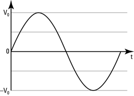
The voltage from an alternating voltage source is not constant — it usually varies like a sine wave. You can see what the voltage from an alternating voltage source looks like in Figure 5-1. The peak voltage — that is, the maximum voltage — is equal to Vo.
Here’s the formula for the voltage from an alternating voltage source as a function of time:
V = Vo sin(2πft)
Here, Vo is the maximum voltage and f is the frequency of the alternating voltage source. Frequency is measured in hertz, whose symbol is Hz. Frequency is the number of complete cycles (from peak to peak along the sine wave, for example) that occur per second.
Figure 5-1: Alternating voltage.
How does this alternating voltage affect Ohm’s law? Not too badly — Ohm’s law just becomes

You can rewrite Ohm’s law in terms of the maximum current, Io, like this (because Vo = Io/R). So here’s Ohm’s law for an AC circuit:

Averaging out: Using root-mean-square current and voltage
When discussing AC circuits, you usually don’t work in terms of maximum voltages and currents, Vo and Io; instead, you speak in terms of the root-mean-square voltages and currents, Vrms and Irms. What’s the difference?
Root-mean-square is a way of treating circuits with alternating voltages much as you’d treat circuits with direct, nonalternating voltages. For example, here’s what the power dissipated as heat in a circuit with nonalternating voltage looks like:
P = IV
And here’s what the dissipated power looks like in a circuit with alternating voltage:
P = IoVo sin2(2πft)
Not exactly the same, are they? So physicists talk in terms of the average power dissipated by a circuit with an alternating current source — that is, averaged over time. That’s a way of looking at alternating-voltage circuits much as you’d look at battery-driven circuits. The time average of sin2(2πft) works out to be 1//2, which is nice, so the average power dissipated by an alternating voltage circuit is

You can also write this as

And that’s where Irms and Vrms come from, because you can also write this as
Pavg = Irms Vrms
where  and
and  .
.
So Irms and Vrms are each the maximum current or voltage, divided by the square root of 2.
Staying in phase: Connecting resistors to alternating voltage sources
Say that you connect an alternating voltage source to a resistor, as Figure 5-2 shows. The circle around the ~ symbol represents an alternating voltage source, and the zigzag represents the resistor.
Figure 5-2: Symbols for an alternating voltage source connected across a resistor with resistance R.

The voltage across the resistor is just the voltage supplied by the alternating voltage source, so the current through the resistor, at time t, is given by Ohm’s law:

Note that if you square both sides of this current-voltage relationship and then take the average (remember that the average of sin2(2πft) works out to be 1//2), then you have a relation between the mean-squared voltage and current. If you take the square root, you get the following relation between the root-mean-square voltage and current across a resistor:
Vrms = Irms R
This is the root-mean-square equivalent of Ohm’s law in an AC circuit.
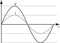
You can see a graph of the current and voltage across the resistor in Figure 5-3. Note that the current through the resistor and the voltage across the resistor rise and fall at the same time. That means that the current and the voltage in a resistor are in phase. (However, the current and voltages through and across capacitors and inductors do not mirror each other — that is, they’re not in phase, as you see later in this chapter.)
Figure 5-3: Voltage and current alternating in a resistor.
AC Circuits and Capacitors: Storing Charge in Electric Field
A capacitor is a device that stores charge when you apply a voltage across it. You may have already met the capacitor in Chapter 3, in the form of two parallel plates. The more charge you put on the plates, the greater the potential difference between them.
Generally, for any type of capacitor, the amount of charge stored for every unit of potential difference is called the capacitance (measured in farads, a unit named after Michael Faraday). The voltage across a capacitor (V) that has capacitance C is related to the amount of charge stored on it (Q) by the following equation:

How does a capacitor react to alternating voltage? That’s what you look at in this section.
Introducing capacitive reactance
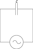
Suppose you connect a capacitor to an alternating voltage source, as Figure 5-4 shows (the symbol for a capacitor is two upright bars, meant to represent the plates of a parallel plate capacitor).
Figure 5-4: An alternating voltage source connected across a capacitor with capacitance C.
Here’s how voltage relates to current when you have a capacitor and an alternating voltage source:
Vrms = Irms Xc
where Vrms and Irms are the root-mean-square voltage and current (the maximum voltage and current divided by the square root of 2 — see the earlier section “Averaging out: Using root-mean-square current and voltage” for details). Here, Xc is called the capacitive reactance, and it’s equivalent to the resistance, R, in the root-mean-square voltage and current relation for the resistor (see the earlier section “Staying in phase: Connecting resistors to alternating voltage sources”). Xc is measured in ohms (Ω), just as R is, and it’s equal to the following:

where f is the frequency of the alternating voltage source and C is the capacitor’s capacitance, measured in farads (F).
 You can think of the capacitive reactance as the effective resistance the capacitor puts in the way of the alternating voltage source, much like R for resistors.
Note that the capacitive reactance depends on frequency, which is something that resistance doesn’t do. When the frequency (f) is low, the capacitive reactance (Xc) is large, and when the frequency is high, the capacitive reactance is small. (The equation shows this relationship by putting f in the bottom of the fraction.)
Why is capacitive reactance high when the frequency is low and low when the frequency is high? Intuitively, you can think of it this way: When the frequency is high, the capacitor doesn’t have much time between voltage reversals to accumulate new charge, so it doesn’t change the voltage across it much. When the frequency is low, the capacitor has more time to accumulate charge during each cycle and so can change its voltage more.
How about seeing some numbers? Say you have a 1.50-μF capacitor (where μF is a microfarad, or 10–6 F), and you connect it across a voltage source whose Vrms = 25.0 volts. What is Irms if the frequency of the voltage source is 100 hertz?
First, find the capacitive reactance:

So the capacitive reactance is 1,060 ohms. Now put that to work finding Irms. You know that Vrms = Irms Xc, so

Plug in the numbers and solve:

And there you have the current — 2.36 × 10⁻² amps. If the frequency were higher, the capacitive reactance would be lower, so the current would be higher (because the capacitive reactance is the effective resistance).
Getting out of phase: Current leads the voltage
When you have a capacitor in an AC circuit, the current and voltage sine waves are out of phase — that is, they’re shifted in time with respect to each other: One reaches its peak before the other. You can see the applied voltage as a function of time in Figure 5-5 — as well as the actual current that flows in the circuit.
Figure 5-5: Alternating voltage and current in a capacitor.
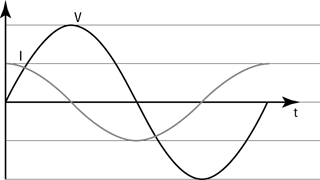
Notice that with a capacitor, the current leads the voltage — that is, the current reaches its peak before the voltage does. In fact, the current leads the voltage by exactly 90°, or π/2 radians — that is, one quarter cycle. So when you’re graphing the current and voltage from a capacitor in an alternating voltage circuit, always remember that the current leads.
Why does current reach its peak before voltage does? The answer is simple if you think about how a capacitor works. Current piles charge onto a capacitor, so as long as the current is positive, the capacitor’s voltage increases. When the current is decreasing in magnitude, it will still be positive for a while, so charge is still being added onto the capacitor; thus, the voltage keeps on increasing. Not until the current changes direction and goes negative does the charge start to come off the capacitor, causing the voltage to decrease. Therefore, the voltage reaches its peak after the current does.
In fact, you say that if the applied voltage is V = Vo sin(2πft), then current, which leads voltage by π/2 radians, looks like this — note that its argument (in parentheses) reaches a specific value before the voltage does because you’re adding π/2 to 2πft:

Using a little trig, this becomes the following:
I = Io cos(2πft)
So you can see that if the voltage goes as the sine, current goes as the cosine, so they’re out of phase.
Preserving power
Here’s something surprising: The average power dissipated by the capacitor is zero. Why? Well, the power used by an electrical component is P = IV. Here’s what this looks like for a resistor, where the current and the voltage are in phase:
P = IoVo sin2(2πft)
However, for a capacitor, the power looks like this, because the current and voltage are 90° out of phase:
P = IoVo sin(2πft) cos(2πft)
The time average of sin(2πft) cos(2πft) is zero (because this product spends as much time positive as it does negative), so the average power used by a capacitor is zero:
Pavg = 0
This means that no power is lost to the environment as heat (as is the case with a resistor), and in fact, the capacitor spends as much time feeding power back into the circuit as it does getting power from the circuit: The capacitor feeds power back to the circuit when it’s discharging and its voltage is going down, and the capacitor gains energy when it’s being charged up and its voltage is increasing.
AC Circuits and Inductors: Storing Energy in Magnetic Field
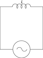
Just as capacitors store energy in an electric field (that is, charges are separated by some distance, giving rise to an electric field), so inductors store energy — but this time, it’s stored in a magnetic field. For example, a solenoid (see Chapter 4) is an inductor, because when you run current through it, a magnetic field appears — and doing that takes energy. In fact, the electrical symbol for an inductor is just that: a solenoid, or loops of current, as you can see in the circuit in Figure 5-6.
Figure 5-6: Adding an inductor with inductance L to a circuit.
Inductors do the same kind of thing as capacitors: They shift the current relative to voltage from an alternating voltage source. However, instead of leading by π/2, the current lags by π/2.
For a capacitor (see the preceding section), the voltage is a function of the capacitance and the charge stored on one plate (the charge stored on one plate is equal in magnitude but opposite in sign to the charge stored on the other plate):

A similar relationship exists for inductors, as you see in this section. Here, I show you how inductors produce a voltage based on the concept of Faraday’s law. For that, I introduce the concept of magnetic flux, which you get when a magnetic field passes through a loop of wire. I also explain how inductive reactance, just like capacitive reactance, opposes an alternating current — only this time, voltage comes out ahead of current.
Faraday’s law: Understanding how inductors work
Michael Faraday (the same physicist that farads, the units of capacitance, are named after), came up with Faraday’s law, which says the following:
When an inductor suffers a change in magnetic flux, it produces a voltage that tends to resist the change.
What does all that mean? This section explains the physics behind inductors, starting with the idea of magnetic flux.
Introducing flux: Magnetic field times area
When a magnetic field goes through a loop of wire, there’s said to be a magnetic flux over the area of the loop. You can see how this works in Figure 5-7. There, a uniform magnetic field (B) is going through a wire loop with area A, which is orientated at an angle θ to the magnetic field.
Figure 5-7: Magnetic flux through a loop of wire.

Here’s where it gets strange: In physics, areas are often represented by vectors, and they point directly out of the flat surface whose area they represent. In other words, the vector B in Figure 5-7 should be familiar — that’s just the magnetic field. But the area vector, A, is new — that’s the vector that’s perpendicular to the wire loop, and its magnitude is the same numerical value as the area of the loop.
Magnetic flux is the strength of the magnetic field multiplied by the component of the area vector parallel to the B field. In other words, magnetic flux is a magnetic field strength multiplied by an area. When the magnetic field is parallel to the area vector, the magnetic flux, whose symbol is Φ, is BA. On the other hand, when B is perpendicular to A, no field lines actually go through the wire loop, and the flux is zero. Putting all this together, here’s what magnetic flux is in terms of B, A, and θ, the angle between them:
Φ = BA cos θ
Inducing a voltage to keep the status quo
Faraday’s law says that if the magnetic flux changes, it induces a voltage around the loop; that voltage creates a current in a way that opposes the change by creating its own magnetic field.
For instance, say that the magnetic field is decreasing in strength. The wire loop wants to keep things the way they are, so it resists change. The wire loop creates a voltage in itself that causes a current to flow — and that current creates a magnetic field.
The magnetic field is created in such a way as to preserve the status quo; thus, the current flows in a way that adds magnetic field to the applied magnetic field — that is, the applied magnetic field is decreasing, so the current around the loop flows to create more magnetic field to replace what’s being decreased. (The inductor can’t keep the current going forever — it dies away quickly, but while it lasts, it creates a magnetic field to supplement the magnetic field that’s decreasing.)
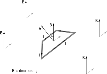
You can see the result in Figure 5-8, which shows the way that the current would flow if the magnetic field B were decreasing. (Tip: Here’s a chance to show off your right-hand rule prowess from Chapter 4. Verify that the direction of the induced current in Figure 5-8 would flow as shown to add more magnetic field to the decreasing applied magnetic field.)
Figure 5-8: An induced current in a loop of wire.
Finding induced voltage using the change in magnetic flux
How is the voltage induced around the loop of wire related to the change in magnetic flux? The voltage looks like this:

That is, the induced voltage is equal to the number of turns in the wire loop (N) multiplied by the change in flux (ΔΦ) divided by the time in which the change in flux takes place (Δt). The negative sign is there to remind you that the induced voltage acts to oppose the change in flux.
Try some numbers here. Say that you have a solenoid consisting of 40 turns of wire, each with an area of 1.5 × 10⁻³ square meters. A magnetic field of 0.050 teslas is perpendicular to each loop of wire (that is, θ = 0°). A tenth of a second later, t = 0.10 s, the magnetic field has increased to 0.060 teslas. What is the induced voltage in the solenoid?
Start by finding the change in flux over a tenth of a second. The flux looks like this for each turn of wire:
Φ = BA cos θ
Therefore, the original flux through each turn of wire is this, bearing in mind that θ = 0° and the original B field is Bo:
Φo = BoA
Putting in numbers gives you the following:
Φo = (0.050 T)(1.5 × 10⁻³ m2) = 7.5 × 10⁻⁵ Wb
Wb stands for weber, the MKS unit of magnetic flux; it’s equal to 1 T-m2.
And the final magnetic flux is equal to this, where Bf is the final magnetic field:
Φf = BfA
Plugging in the numbers gives you the following:
Φo = (0.060 T)(1.5 × 10⁻³ m2) = 9.0 × 10⁻⁵ Wb
So the change in flux is
ΔΦ = Φf – Φo
= 9.0 × 10⁻⁵ Wb – 7.5 × 10⁻⁵ Wb
= 1.5 × 10⁻⁵ Wb
This change takes place in 0.10 seconds, and it takes place in all 40 turns
of the solenoid, so the equation  becomes
 .
.
So there you have it — the voltage the solenoid creates to oppose the change in magnetic flux is 6.0 mV (millivolts). That’s what the induced voltage starts off at — it decays exponentially in time.
Finding induced voltage using the change in current
The voltage induced by an inductor looks like this:

However, if you have an electrical inductor — that is, a component in a circuit — you don’t typically talk in terms of the change in flux inside that component. Instead, you talk about the change in current through the inductor, because that makes more sense in the context of circuits than speaking of magnetic flux.
How do you relate current through the solenoid and magnetic flux? Plugging in Φ = BA cos θ gives you the following:

And for a solenoid, B = μonI, where n is the number of wire loops in the solenoid per meter — that is, the number of turns per meter — μo is 4π × 10–7 T•m/A, and I is the current in each turn (see Chapter 4 for details). Also, because you have only one selenoid, with n turns per meter, then N = 1. So you can write the voltage as

If the current is the only thing changing in an inductor that’s part of an electric circuit, you get this:

You wrap μonA cos θ up into one number — the inductance of the inductor, whose symbol is L, and whose units are henries (which my friend Henry thinks is a good idea). So you have this equation to tie the induced voltage to the change in current over time:

That’s the result you’re looking for — the inductance connects the change in current over time to the induced voltage. And so all inductors you see in circuits are labeled with their inductance in henries (H).
Introducing inductive reactance
For a resistor, voltage and current relate like this: Vrms = Irms R. And for a capacitor, you have Vrms = Irms Xc, where Xc is the capacitive reactance:

So it shouldn’t surprise you that for an inductor, you have another formula that relates root-mean-square voltage and current — the maximum voltage and current divided by the square root of 2 (for more on these terms, see the earlier section “Averaging out: Using root-mean-square current and voltage”):
Vrms = Irms XL
where XL is the inductive reactance — that is, the effective resistance of the inductor: XL = 2πfL.
Note that capacitive reactance gets big when the frequency of the applied voltage gets low, but inductive reactance gets big when the frequency gets big — opposite to capacitors. Why is this? It’s because inductors act to oppose any change in the magnetic fields inside them. And the faster the applied voltage changes, the larger the change in flux divided by time — which means that the induced voltage can get really large when you go to a very high frequency.
Check out an example using inductive reactance. Say that you have an inductor with an inductance of L = 3.60 mH (millihenries), and you apply a voltage with a root-mean-square value of 25.0 volts across it at 100 hertz. What’s the induced current in the inductor? Starting with Vrms = Irms XL, you see that

You know Vrms, so you need to figure out XL:
XL = 2πfL
Putting in the numbers you know gives you the following:
XL = 2π(100 Hz)(3.60 × 10⁻³ H) ≈ 2.26 Ω
And plugging this into the equation for Irms gives you the answer:
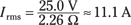
So you’d get a pretty hefty 11-amp induced current.
Getting behind: Current lags voltage
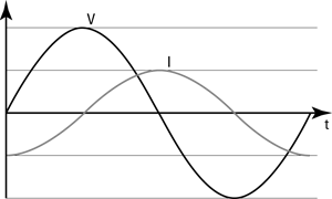
How does the current in an inductor behave when you apply an alternating voltage? You can see the result in Figure 5-9, which graphs the current and the voltage in an inductor as a function of time. Note that here, current lags voltage — the opposite behavior from a capacitor, where current leads voltage. When current lags voltage, voltage reaches its peak before current does.
Figure 5-9: Current lags voltage in an inductor.
Why does current lag voltage in an inductor? It’s because of the following relation:

Note that this equation means that the voltage is greatest when the current is changing the fastest, because the voltage is directly proportional to the rate of change in current. So when the current is the steepest — when current is changing from negative to positive — it’s changing the fastest, and voltage reaches its highest point. Conversely, when current is flat, it’s not changing much at all, so the voltage goes to zero.
As you may expect, current lags voltage by exactly 90° — that is, π/2 in radians. So if the voltage is V = Vo sin(2πft), then current, which lags voltage by 90°, looks like this:

Using a little trig, this becomes the following:
I = –Io cos(2πft)
So that means that for an inductor, the power looks like this, because the current and voltage are 90° out of phase:
P = –IoVo sin(2πft) cos(2πft)
Note that, just as for a capacitor, the time average of sin(2πft) cos(2πft) is zero, so the average power used by an inductor is zero:
Pavg = 0
The Current-Voltage Race: Putting It Together in Series RLC Circuits
Suppose you put a resistor, a capacitor, and an inductor together in the same circuit. The circuit in Figure 5-10 is called a series RLC circuit — series because all components are connected in series, one after the other (the same current has to flow through all of them) and RLC because it’s a resistor-inductor-capacitor circuit (sometimes also called an RCL circuit). Note that the behavior of this circuit doesn’t depend on the order of the circuit elements, so RLC or CLR would be just as good of a name.
 Why doesn’t the order of a resistor, inductor, and capacitor matter in a circuit? Consider the potential difference across each element: Across the resistor, the potential difference depends only on the current; across the inductor, it depends on only the rate of change of the current; and across the capacitor, it depends only on the sum of the current over time (that is, the charge). So the potential difference across each element depends only on the current, and the same current always flows through each in series, whatever order they’re in.
Figure 5-10: A series RLC circuit.

All the components are fighting each other over whether the voltage leads or lags — the capacitor wants the current to lead the voltage, the inductor wants the current to lag the voltage, and the resistor wants the voltage and the current to be in phase. Who wins? This section tells you where to place your bets.
Impedance: The combined effects of resistors, inductors, and capacitors
Earlier in this chapter, you see the relationship between root-mean-square current and voltage for the resistor, the inductor, and the capacitor. When you have a circuit combining various elements like resistors, capacitors, and inductors, then there’s a similar relation for the circuit as a whole. The root-mean-square voltage across the circuit, per unit of root-mean-square current, is called the impedance.
Phasor diagrams: Pointing out alternating voltage and current
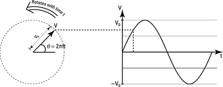
To tackle the problem of alternating voltages in an RLC circuit, you get a new tool: the phasor diagram. In this diagram, you represent the various alternating quantities as an arrow that rotates in time — you can see how this works in Figure 5-11:
The arrow (phasor) on the left represents the alternating voltage V, with amplitude V0. The length of the arrow is V0.
The arrow’s angle from the horizontal, θ, is called the phase.
Now if you allow this arrow, initially horizontal, to rotate at a constant frequency f, then the phase is θ = 2πft. As you can see in Figure 5-11, if you project horizontally from the phasor at time t, then you get the value V0 sin θ, which is just an alternating voltage. You can represent the current in the same way with its own arrow. If the current leads the voltage by 90°, for example, then its phasor is rotated 90° further clockwise.
Figure 5-11: A phasor diagram of an alternating voltage.
Adding phasors and finding impedance
In Figure 5-12a, you can see three phasors representing the voltages across the resistor (VR), inductor (VL), and capacitor (VC) in a circuit. In this figure, they’re shown at time t, when the phase of the voltage across the resistor is θ = 2πft. Notice the voltage across the inductor leads the voltage across the resistor by 90°, and the capacitor lags by 90°.
Figure 5-12: (a) Relative angles of voltages in the resistor, inductor, and capacitor; (b) The total voltage across the resistor, inductor, and capacitor.
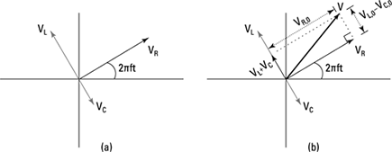
The total potential difference across all the circuit elements, V, is just the sum of the potential difference across each element. So to find V, add the phasors using vector addition (see Chapter 2 for info on adding vectors). Now, because VL and VC are always 180° out of phase, they simply point in opposite directions, so their sum is a new vector whose length is the difference in the amplitude of these two voltages.
The direction of this new phasor (VL + VC) is still 90° from VR, because you’ve added two phasors that are both 90° from the phasor of VR. To get the total sum, add VR to this new phasor. You can see the sum of the voltages in Figure 5-12b. Because the phasors are at right angles, you can use the Pythagorean theorem to find the resulting length. The squared length of the sum of the potential differences is
V02 = (VR,0)2 + (VL,0 – VC,0)2
where V0, VR,0 , and VC,0 are the amplitudes of the voltages.
Now if you use the relation between the amplitude V0 and the root-mean-square voltage Vrms, you can use this to write the root-mean-square total voltage as
Vrms2 = VR,rms2 + (VL,rms – VC,rms)2
where VR,rms, VL,rms, and VC,rms are root-mean-square voltages across the resistor, inductor, and capacitor respectively.
To simplify this equation, recognize that the following equations are true (note that because the current flows through all the components in series, only one current, Irms, is in the circuit):
VR,rms = Irms R
VC,rms = Irms XC
VL,rms = Irms XL
Therefore, you can put the equations together and solve for Vrms:
Vrms2 = Irms2 [R2 + (XL – XC)2]
Vrms = Irms [R2 + (XL – XC)2]1/2
Now you’re getting somewhere — you have Vrms in terms of Irms. This equation has the form
Vrms = Irms Z
where Z = [R2 + (XL – XC)2]1/2. Very nice. Now you’ve connected Vrms to Irms with this new quantity, Z. Z is called the impedance of the whole series RLC circuit, and it functions like the effective resistance of the whole RLC circuit.
Determining the amount of leading or lagging
For a series RLC circuit, Vrms = Irms Z (see the preceding section to find out where this equation comes from). That connects Vrms and Irms in terms of their magnitude. But which leads — voltage or current? And by how much?
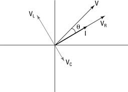
Look at a voltages-as-vectors graph. In Figure 5-13, I’ve added I (which is in phase with the voltage across the resistor, so it overlaps VR) as a thick vector.
The question of whether voltage or current leads becomes, “What’s the angle θ (as shown in the figure) between V and I?” Here’s why:
If that angle is positive, the net result of all three components is that the voltage leads the current.
If that angle is negative, voltage lags the current.
Figure 5-13: The angle between I and V.
According to the figure, the tangent of this angle is
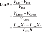
Note that in the second line, I’ve used the fact that the root-mean-square voltage is just the amplitude divided by the square root of 2; then I canceled the square root of 2 from the top and bottom of the fraction. Canceling out Irms in the last line gives you

So take the inverse tangent, tan–1, to find θ:

That’s the angle by which voltage leads or lags the current across all three elements. If θ = 0°, the voltage is in phase with the current — the effects of the inductor cancel out those of the capacitor. If it’s positive, the inductor is winning; if it’s negative, the capacitor is winning.
Finding the root-mean-square current
How about some numbers? Say that you have a circuit consisting of a 148-ohm resistor, a 1.50-microfarad capacitor, and a 35.7-millihenry inductor. The circuit is driven by an alternating voltage source with a root-mean-square voltage of 35.0 volts at 512 hertz. What is the root-mean-square current through the circuit, and by how much does the current lead or lag the voltage?
Start by getting the reactance of the capacitor and the inductor. They look like this:
Capacitor: 
Inductor: XL = 2πfL = 2π(512 Hz)(35.7 × 10⁻³ H) ≈ 115 Ω
The impedance is
Z = [R2 + (XL – Xc)2]1/2
Plugging in the numbers for resistance, inductive reactance, and capacitive reactance gives you the following:
Z = [148 Ω2 + (115 Ω – 207 Ω)2]1/2 ≈ 174 Ω
And because  , you get the following answer for the current:

Quantifying the leading or lagging
Now, does the root-mean-square current lead or lag the voltage? In this example, the capacitive reactance (207 ohms) is greater than the inductive reactance (115 ohms), so you can say that the capacitor wins here and the voltage lags the current. But by how much?
Take the following equation:

Just plug in the numbers. Because the resistance is 148 ohms, you find that

So take the inverse tangent to find the angle:
θ = tan–1(–0.62) ≈ –32°
And there you have it — voltage does indeed lag the current, just as in a capacitor.
Peak Experiences: Finding Maximum Current in a Series RLC Circuit
Earlier in this chapter, the resistor, capacitor, and inductor all have fixed values, as does the applied voltage. But all those things can vary: You can use electrical components that let you vary their resistance, their capacitance, their inductance, their voltage — even the frequency of that voltage. If you’re going to vary anything in an RLC circuit, varying the frequency is the most common choice. This section tells you how to find the frequency at which you get the most current.
Canceling out reactance
When you let various quantities vary in an RLC circuit, the amount of current through the circuit changes. Because Vrms = Irms Z, where Z = [R2 + (XL – Xc)2]1/2, you have the following:

Note that the current through the circuit (Irms) will reach a maximum when Z, the impedance, reaches a minimum — that is, when Z is at its smallest value. Because Z = [R2 + (XL – Xc)2]1/2, impedance will reach its minimum value when the inductive reactance equals the capacitive reactance:
XL = Xc
At that point, Z = R.
Note that in this case, when the circuit is in resonance and the effects of the inductor and capacitor cancel each other out, the current and voltage are in phase.
Finding resonance frequency
The frequency at which the current reaches its maximum value is called the resonance frequency. At the resonance frequency, the effects of the capacitor and the inductor cancel out, leaving the resistor as the only effective element in the circuit.
What is the resonance frequency for any given RLC circuit? You know that
 and XC = 2πfL.
At the resonance frequency fres, the inductive reactance and capacitive reactance are equal, so the following equation holds:

Rearranging this equation and solving for frequency gives you

And there you have it — that’s the frequency at which the current reaches its maximum value for any given L and C values.
Semiconductors and Diodes: Limiting Current Direction
One of the great leaps of the technological age happened when people started combining the resistor and the capacitor with some new circuit elements made from materials that were semiconductors. The combination was an extremely powerful one. These circuits, combining resistors, capacitors, and semiconductor devices, eventually became miniaturized into integrated circuits, or microchips, which form the basis for many devices that have changed the way people live — most notably the computer. (So the next time someone complains you’re spending too much time on the computer, tell them you’re doing physics.)
In this section, I first introduce semiconductors so you understand their special properties. Then I introduce an example of a circuit element made from them: the diode. This simple device allows current to pass through it in one direction only — it’s effectively a one-way valve for electrical current.
The straight dope: Making semiconductors
Normal silicon (Si) has a crystalline structure, with four electrons from each atom taking part in bonding each atom to its neighbors. Those electrons are in the outermost orbits of the silicon atom, and because they’re important in creating the crystalline structure, they’re not available to conduct electricity — hence, normal silicon is an insulator.
But by being clever, you can introduce small amounts of impurities (such as one part in a million) that give the silicon conducting properties. Here are two types of semiconductors you can create:
N-type semiconductors: Adding some phosphorus (P) atoms allows the silicon to conduct electricity. Phosphorus has five electrons in its outermost orbit, so when you dope silicon with phosphorus, the phosphorus atoms join the silicon crystal structure, which binds each atom to its neighbors using four electrons. That means that there’s one electron from the phosphorus left over — and that electron is free to roam.
The resulting doped silicon is called an n-type semiconductor, because the charges that carry current in it — the electrons contributed by the phosphorus — are negative.
P-type semiconductors: On the other hand, you can dope silicon with other elements, such as boron (B), which has only three outer electrons per atom. When the boron binds to the silicon-crystal structure, one electron is missing, so there’s a “hole” in the number of electrons.
That hole can move from atom to atom — and each hole produces a positive charge, because it’s formed from a deficit of electrons. Because the holes (that is, the localized places where you have a missing electron) can move throughout the semiconductor, the charge-carriers in this kind of doped silicon are positive. When you have a material with mobile holes, it’s called a p-type semiconductor, because the free charge-carriers are positive.
That’s the whole charm of semiconductors — in addition to negatively charged carriers (electrons), you can also have positively charged carriers (the holes).
One-way current: Creating diodes
You can create diodes — one-way current valves — by putting some p-type semiconductor next to some n-type semiconductor (see the preceding section for info on types of semiconductors). In the case at the top of Figure 5-14, voltage is applied with the positive voltage connected to the p-type semiconductor, and negative voltage is connected to the n-type semiconductor.
In this case, charge flows freely across the junction between the p-type and n-type semiconductors, because the positive holes on the left are repelled from the positive terminal and travel to the right, and the electrons on the right are repelled by the negative terminal, so they travel to the left. The holes and electrons meet at the junction, and the electrons fill the holes — so current can flow. The negative terminal provides more electrons for this process, and the positive terminal removes them, creating more holes.
Figure 5-14: Semi-conductor diodes at work.

On the other hand, if you reverse the terminals of the battery, no current will flow through the diode, as the bottom of Figure 5-14 shows. That’s because in this case, the battery drives the mobile charge-carriers away from the junction. As you can see in the figure, the positive holes travel to the left in the p-type semiconductor — away from the junction — and the electrons in the n-type semiconductor travel to the right, also away from the junction.
What’s left at the junction are the immobile negative charges in the p-type material and the immobile positive charges in the n-type material. Those charges don’t move, so they set up an electric field that counteracts the electric field set up by the battery — with the net result that all current stops.