Chapter 3

Exploring the Need for Speed

In This Chapter

Getting up to speed on displacement

Dissecting different kinds of speed

Going with acceleration

Examining the link among acceleration, time, and displacement

Connecting velocity, acceleration, and displacement

There you are in your Formula 1 racecar, speeding toward glory. You have the speed you need, and the pylons are whipping past on either side. You’re confident that you can win, and coming into the final turn, you’re far ahead. Or at least you think you are. Seems that another racer is also making a big effort, because you see a gleam of silver in your mirror. You get a better look and realize that you need to do something — last year’s winner is gaining on you fast.

It’s a good thing you know all about velocity and acceleration. With such knowledge, you know just what to do: You floor the gas pedal, accelerating out of trouble. Your knowledge of velocity lets you handle the final curve with ease. The checkered flag is a blur as you cross the finish line in record time. Not bad. You can thank your understanding of the issues in this chapter: displacement, velocity, and acceleration.

You already have an intuitive feeling for what I discuss in this chapter, or you wouldn’t be able to drive or even ride a bike. Displacement is about where you are, speed is about how fast you’re going, and anyone who’s ever been in a car knows about acceleration. These characteristics of motion concern people every day, and physics has made an organized study of them. This knowledge has helped people to plan roads, build spacecraft, organize traffic patterns, fly, track the motion of planets, predict the weather, and even get mad in slow-moving traffic jams. Understanding movement is a vital part of understanding physics, and that’s the topic of this chapter. Time to move on.

Going the Distance with Displacement

When something moves from Point A to Point B, displacement takes place in physics terms. In plain English, displacement is a distance in a particular direction.

Like any other measurement in physics (except for certain angles), displacement always has units — usually centimeters or meters. You may also use kilometers, inches, feet, miles, or even light-years (the distance light travels in one year, a whopper of a distance not fit for measuring with a meter stick: 5,865,696,000,000 miles, which is 9,460,800,000,000 kilometers or 9,460,800,000,000,000 meters).

In this section, I cover position and displacement in one to three dimensions.

Understanding displacement and position

You find displacement by finding the distance between an object’s initial position and its final position. Say, for example, that you have a fine new golf ball that’s prone to rolling around, shown in Figure 3-1. This particular golf ball likes to roll around on top of a large measuring stick. You place the golf ball at the 0 position on the measuring stick, as you see in Figure 3-1, diagram A.

Figure 3-1: Examining displacement with a golf ball.

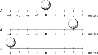
The golf ball rolls over to a new point, 3 meters to the right, as you see in Figure 3-1, diagram B. The golf ball has moved, so displacement has taken place. In this case, the displacement is just 3 meters to the right. Its initial position was 0 meters, and its final position is at +3 meters. The displacement is 3 meters.

In physics terms, you often see displacement referred to as the variable s (don’t ask me why).

Scientists, being who they are, like to go into even more detail. You often see the term si, which describes initial position, (the i stands for initial). And you may see the term sf used to describe final position.

In these terms, moving from diagram A to diagram B in Figure 3-1, si is at the 0-meter mark and sf is at +3 meters. The displacement, s, equals the final position minus the initial position:

s = sf – si

= 3 m – 0 m = 3 m

Displacements don’t have to be positive; they can be zero or negative as well. If the positive direction is to the right, then a negative displacement means that the object has moved to the left.

In diagram C, the restless golf ball has moved to a new location, which is measured as –4 meters on the measuring stick. The displacement is given by the difference between the initial and final position. If you want to know the displacement of the ball from its position in diagram B, take the initial position of the ball to be si = 3 meters; then the displacement is given by

s = sf – si

= –4 m – 3 m = –7 m

When working on physics problems, you can choose to place the origin of your position-measuring system wherever is convenient. The measurement of the position of an object depends on where you choose to place your origin; however, displacement from an initial position si to a final position sf does not depend on the position of the origin because the displacement depends only on the difference between the positions, not the positions themselves.

Examining axes

Motion that takes place in the world isn’t always in one dimension. Motion can take place in two or three dimensions. And if you want to examine motion in two dimensions, you need two intersecting meter sticks (or number lines), called axes. You have a horizontal axis — the x-axis — and a vertical axis — the y-axis. (For three-dimensional problems, watch for a third axis — the z-axis — sticking straight up out of the paper.)

Finding the distance

Take a look at Figure 3-2, where a golf ball moves around in two dimensions. The ball starts at the center of the graph and moves up to the right. In terms of the axes, the golf ball moves to +4 meters on the x-axis and +3 meters on the y-axis, which is represented as the point (4, 3); the x measurement comes first, followed by the y measurement: (x, y).

So what does this mean in terms of displacement? The change in the x position, Δx (Δ, the Greek letter delta, means “change in”), is equal to the final x position minus the initial x position. If the golf ball starts at the center of the graph — the origin of the graph, location (0, 0) — you have a change in the x location of

Δx = xf – xi

= 4 m – 0 m = 4 m

The change in the y location is

Δy = yf – yi

= 3 m – 0 m = 3 m

Figure 3-2: A ball moving in two dimensions.

If you’re more interested in figuring out the magnitude (size) of the displacement than in the changes in the x and y locations of the golf ball, that’s a different story. The question now becomes: How far is the golf ball from its starting point at the center of the graph?

Using the distance formula — which is just the Pythagorean theorem solved for the hypotenuse — you can find the magnitude of the displacement of the golf ball, which is the distance it travels from start to finish. The Pythagorean theorem states that the sum of the squares of the legs of a right triangle (a2 + b2) is equal to the square on the hypotenuse (c2). Here, the legs of the triangle are Δx and Δy, and the hypotenuse is s. Here’s how to work the equation:

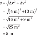
So in this case, the magnitude of the ball’s displacement is exactly 5 meters.

Determining direction

You can find the direction of an object’s movement from the values of Δx and Δy. Because these are just the legs of a right triangle, you can use basic trigonometry to find the angle of the ball’s displacement from the x-axis. The tangent of this angle is simply given by

Therefore, the angle itself is just the inverse tangent of that:

The ball in Figure 3-2 has moved at an angle of 37° from the x-axis.

Speed Specifics: What Is Speed, Anyway?

There’s more to the story of motion than just the actual movement. When displacement takes place, it happens in a certain amount of time. You may already know that speed is distance traveled per a certain amount of time:

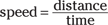
For example, if you travel distance s in a time t, your speed, v, is

The variable v really stands for velocity, but true velocity also has a direction associated with it, whereas speed does not. For that reason, velocity is a vector (you usually see the velocity vector represented as v or . Vectors have both a magnitude (size) and a direction, so with velocity, you know not only how fast you’re going but also in what direction. Speed is only a magnitude (if you have a certain velocity vector, in fact, the speed is the magnitude of that vector), so you see it represented by the term v (not in bold). You can read more about velocity and displacement as vectors in Chapter 4.

Just as you can measure displacement, you can measure the difference in time from the beginning to the end of the motion, and you usually see it written like this: Δt = tf – ti. Technically speaking (physicists love to speak technically), velocity is the change in position (displacement) divided by the change in time, so you can also represent it like this, if, say, you’re moving along the x-axis:

Speed can take many forms, which you find out about in the following sections.

Reading the speedometer: Instantaneous speed

You already have an idea of what speed is; it’s what you measure on your car’s speedometer, right? When you’re tooling along, all you have to do to see your speed is look down at the speedometer. There you have it: 75 miles per hour. Hmm, better slow it down a little — 65 miles per hour now. You’re looking at your speed at this particular moment. In other words, you see your instantaneous speed.

Instantaneous speed is an important term in understanding the physics of speed, so keep it in mind. If you’re going 65 mph right now, that’s your instantaneous speed. If you accelerate to 75 mph, that becomes your instantaneous speed. Instantaneous speed is your speed at a particular instant of time. Two seconds from now, your instantaneous speed may be totally different.

Staying steady: Uniform speed

What if you keep driving 65 miles per hour forever? You achieve uniform speed in physics (also called constant speed). Uniform motion is the simplest speed variation to describe, because it never changes.

Uniform speed may be possible in the western portion of the United States, where the roads stay in straight lines for a long time and you don’t have to change your speed. But uniform speed is also possible when you drive around a circle, too. Imagine driving around a racetrack; your velocity would change (because of the constantly changing direction), but your speed could remain constant as long as you keep your gas pedal pressed down the same amount. I discuss uniform circular motion in Chapter 7, but in this chapter, I stick to motion in straight lines.

Shifting speeds: Nonuniform motion

Nonuniform motion varies over time; it’s the kind of speed you encounter more often in the real world. When you’re driving, for example, you change speed often, and your changes in speed come to life in an equation like this, where vf is your final speed and vi is your initial speed:

Δv = vf – vi

The last part of this chapter is all about acceleration, which occurs in nonuniform motion. There, you see how changing speed is related to acceleration — and how you can accelerate even without changing speed!

Busting out the stopwatch: Average speed

Average speed is the total distance you travel divided by the total time it takes. Average speed is sometimes written as ; a bar over a variable means average in physics terms.

Say, for example, that you want to pound the pavement from New York City to Los Angeles to visit your uncle’s family, a distance of about 2,781 miles. If the trip takes you 4.000 days, what was your average speed? You divide the total distance by the change in time, so your average speed for the trip would be

This solution divides miles by days, so you come up with 695.3 miles per day. Not exactly a standard unit of measurement — what’s that in miles per hour? To find it, you want to cancel days out of the equation and put in hours (see Chapter 2). Because a day is 24 hours, you can multiply this way (note that days cancels out, leaving miles over hours, or miles per hour):

That’s a better answer.

You can relate total distance traveled, s, with average speed, , and time, t, like this:

Contrasting average and instantaneous speed

Average speed differs from instantaneous speed, unless you’re traveling in uniform motion (in which case your speed never varies). In fact, because average speed is the total distance divided by the total time, it may be very different from your instantaneous speed.

If you travel 2,781 miles in four days (a total of 96 hours), you go at an average speed of 28.97 miles per hour. That answer seems pretty slow, because when you’re driving, you’re used to going 65 miles per hour. You’ve calculated an average speed over the whole trip, obtained by dividing the total distance by the total trip time, which includes non-driving time. You may have stopped at a hotel several nights, and while you slept, your instantaneous speed was 0 miles per hour; yet even at that moment, your overall average speed was still 28.97 miles per hour!

Distinguishing average speed and average velocity

There is a difference between average speed and average velocity. Say, for example, that while you were driving in Ohio on your cross-country trip, you wanted to make a detour to visit your sister in Michigan after you dropped off a hitchhiker in Indiana. Your travel path may have looked like the straight lines in Figure 3-3 — first 80 miles to Indiana and then 30 miles to Michigan.

If you drove at an average speed or a uniform speed of 55 miles per hour and you had to cover 80 + 30 = 110 miles, this trip took you 2.0 hours. But if you calculate the magnitude of the average velocity (by taking the distance between the starting point and the ending point, about 85 miles as the crow flies), you get

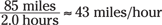
Figure 3-3: A trip from Ohio to Michigan.

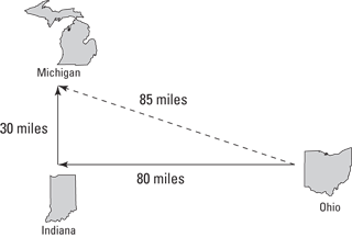
The direction of the average velocity is just the direction between the start and end points. But if you’re interested in your average speed along either of the two legs of the trip, you have to measure the time it takes for a leg and divide the length of that leg by that time to get the average speed.

To calculate the average speed over the whole trip, you look at the whole distance traveled, which is 80 + 30 = 110 miles, not just 85 miles. And 110 miles divided by 2.0 hours is 55 miles per hour; this is your average speed.

As another illustration of the difference between average speed and average velocity, consider the motion of the Earth around the sun. The Earth travels in its nearly circular orbit around the sun at an enormous average speed of something like 18 miles per second! However, if you consider one full revolution of the Earth, the Earth returns to its original position, relative to the sun, after one year. After one year, there’s no displacement relative to the sun, so the Earth’s average velocity over a year is zero, even though its average speed is enormous!

When considering motion, it’s not only speed that counts but also direction. That’s why velocity is important: It lets you record an object’s speed and its direction. Pairing speed with direction enables you to handle cases like cross-country travel, where the direction can change.

Speeding Up (Or Down): Acceleration

Acceleration is a measure of how quickly your velocity changes. When you pass a parking lot’s exit and hear squealing tires, you know what’s coming next — someone is accelerating to cut you off. After he passes, he slows down right in front of you, forcing you to hit your brakes to slow down yourself. Good thing you know all about physics.

You may think that, with all this speeding up and slowing down, you’d use terms like acceleration and deceleration. Well, physics has no use for the term deceleration, because deceleration is just a particular kind of acceleration — one in which speed reduces.

Like speed, acceleration takes many forms that affect your calculations in various physics situations. In different physics problems, you have to take into account the direction of the acceleration (whether the acceleration is positive or negative in a particular direction), whether it’s average or instantaneous, and whether it’s uniform or nonuniform. This section tells you more about acceleration and explores its various forms.

Defining acceleration

In physics terms, acceleration, a, is the amount by which your velocity changes in a given amount of time, or

Given the initial and final velocities, vi and vf, and the initial and final times over which your speed changes, ti and tf, you can also write the equation like this:

Acceleration, like velocity, is actually a vector and is often written as a, in vector style (see Chapter 4). In other words, acceleration, like velocity but unlike speed, has a direction associated with it.

Determining the units of acceleration

You can calculate the units of acceleration easily enough by dividing velocity by time to get acceleration:

In terms of units, the equation looks like this:

Distance per time squared? Don’t let that throw you. You end up with time squared in the denominator because you divide velocity by time. In other words, acceleration is the rate at which your velocity changes, because rates have time in the denominator. For acceleration, you see units of meters per second2, centimeters per second2, miles per second2, feet per second2, or even kilometers per hour2.

It may be easier, for a given problem, to use units such as mph/s (miles per hour per second). This would be useful if the velocity in question had a magnitude of something like several miles per hour that changed typically over a number of seconds.

Looking at positive and negative acceleration

Just as for displacement and velocity, acceleration can be positive or negative. This section explains how positive and negative acceleration relate to changes in speed and direction.

Changing speed

The sign of the acceleration tells you whether you’re speeding up or slowing down (depending on which direction you’re traveling).

For example, say that you’re driving at 75 miles per hour, and you see those flashing red lights in the rearview mirror. You pull over, taking 20 seconds to come to a stop. The officer appears by your window and says, “You were going 75 miles per hour in a 30-mile-per-hour zone.” What can you say in reply?

You can calculate your rate of acceleration as you pulled over, which, no doubt, would impress the officer — look at you and your law-abiding tendencies! You whip out your calculator and begin entering your data. Remember that the acceleration is given in terms of the change in velocity divided by the change in time:

Plugging in the numbers, your calculations look like this:

Your acceleration was 3.8 mph/s. But that can’t be right! You may already see the problem here; take a look at the original definition of acceleration:

Your final speed was 0 mph, and your original speed was 75 mph, so plugging in the numbers here gives you this acceleration:

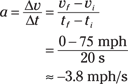
In other words, –3.8 mph/s, not +3.8 mph/s — a big difference in terms of solving physics problems (and in terms of law enforcement). If you accelerated at +3.8 mph/s rather than –3.8 mph/s , you’d end up going 150 mph at the end of 20 seconds, not 0 mph. And that probably wouldn’t make the cop very happy.

Now you have your acceleration. You can turn off your calculator and smile, saying, “Maybe I was going a little fast, officer, but I’m very law abiding. Why, when I heard your siren, I accelerated at –3.8 mph/s just in order to pull over promptly.” The policeman pulls out his calculator and does some quick calculations. “Not bad,” he says, impressed. And you know you’re off the hook.

Accounting for direction

The sign of the acceleration depends on direction. If you slow down to a complete stop in a car, for example, and your original velocity was positive and your final velocity was 0, then your acceleration is negative because a positive velocity came down to 0. However, if you slow down to a complete stop in a car and your original velocity was negative and your final velocity was 0, then your acceleration would be positive because a negative velocity increased to 0.

Looking at positive and negative acceleration

When you hear that acceleration is going on in an everyday setting, you typically think that means the speed is increasing. However, in physics, that isn’t always the case. An acceleration can cause speed to increase, decrease, and even stay the same!

Acceleration tells you the rate at which the velocity is changing. Because the velocity is a vector, you have to consider the changes to its magnitude and direction. The acceleration can change the magnitude and/or the direction of the velocity. Speed is only the magnitude of the velocity.

Here’s a simple example that shows how a simple constant acceleration can cause the speed to increase and decrease in the course of an object’s motion.Say you take a ball, throw it straight up in the air, and then catch it again. If you throw the ball upward with a speed of 9.8 m/s, the velocity has a magnitude of 9.8 m/s in the upward direction. Now the ball is under the influence of gravity, which, on the surface of the Earth, causes all free-falling objects to undergo a vertical acceleration of –9.8 m/s2. This acceleration is negative because its direction is vertically downward.

With this acceleration, what’s the velocity of the ball after 1.0 second ? Well, you know that

Rearrange this equation and plug in the numbers, and you find that the final velocity after 1.0 second is 0 meters/second:

vf = vi + a(tf – ti)

= 9.8 m/s + (–9.8 m/s2 )(1.0 s)

= 0 m/s

After 1.0 second, the ball has zero velocity because it’s reached the top of its trajectory, just at the point where it’s about to fall back down again. So the acceleration has actually slowed down the ball because it was going in the direction opposite the velocity.

Now see what happens as the ball falls back down to Earth. The ball has zero velocity, but the acceleration due to gravity accelerates the ball downward at a rate of –9.8 m/s2. As the ball falls, it gathers speed before you catch it. What’s its final velocity as you catch it, given that its initial velocity at the top of its trajectory is zero?

The time for the ball to fall back down to you is just the same as the time it took to reach the top of its trajectory, which is 1.0 second, so you can find the final velocity for this part of the ball’s motion with this calcuation:

vf = vi + a(tf – ti)

= 0 m/s + (–9.8 m/s2 )(1.0 s)

= –9.8 m/s

So the final velocity is 9.8 meters/second directed straight downward. The magnitude of this velocity — that is, the speed of the ball — is 9.8 meters/second. The acceleration increases the speed of the ball as it falls because the acceleration is in the same direction as the velocity for this part of the ball’s trajectory.

When you work with physics problems, bear in mind that acceleration can speed up or slow down an object, depending on the direction of the acceleration and the velocity of the object. Don’t simply assume that just because something is accelerating its speed must be increasing. (By the way, if you want to see an example of how an acceleration can leave the speed of an object unchanged, take a look at the circular motion topic covered in Chapter 7.)

Examining average and instantaneous acceleration

Just as you can examine average and instantaneous speeds and velocities, you can also examine average and instantaneous acceleration. Average acceleration is the ratio of the change in velocity to the change in time. You calculate average acceleration, also written as , by taking the final velocity, subtracting the initial velocity, and dividing the result by the total time (final time minus the initial time):

At any given point, the acceleration you measure is the instantaneous acceleration, and that number can be different from the average acceleration. For example, when you first see red flashing police lights behind you, you may jam on the brakes, which gives you a big acceleration, in the direction opposite to which you’re moving (in everyday parlance, you’d say you just decelerated, but that term’s a no-no in physics circles). But you lighten up a little and coast to a stop, so the acceleration is smaller. The average acceleration, however, is a single value, derived by dividing the overall change in velocity by the overall time.

Acceleration is the rate of change of velocity, not speed. If a velocity’s direction changes without a change in speed, this is also a kind of acceleration.

Taking off: Putting the acceleration formula into practice

Here’s an acceleration example. As they strap you into the jet on the aircraft carrier deck, the mechanic says you need to take off at a speed of at least 62.0 m/s. You’ll be catapulted at an acceleration of 31 m/s2. Is there going to be enough catapult to do the job? You ask how long the catapult is. “A hundred meters,” says the mechanic, finishing strapping you in.

Hmm, you think. Will an acceleration of 31 m/s2 over a distance of 100 meters do the trick? You take out your clipboard and ask yourself: How far must I be accelerated at 31 m/s2 to achieve a speed of 62 m/s?

First think of the distance that you need to be accelerated over as the size of the displacement from your initial position. To find this displacement, you can use the equation , where s is the displacement, is the average velocity, and t is the time — which means you have to find the time over which you’re accelerated. For that, you can use the equation that relates change in velocity, Δv, acceleration a, and change in time, Δt:

Solving for Δt gives you

Plugging in the numbers and solving gives you the change in time:

Okay, so it takes 2.0 seconds for you to reach a speed of 62 m/s if your rate of acceleration is 31 m/s2. Now you can use this equation to find the total distance you need to travel to get up to this speed; it is the size of the displacement, which is given by , where , vi = 0 m/s, and vf = 62 m/s. So your equation is

Plugging in the numbers gives you

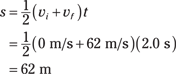
So it will take 62 meters of 31 m/s2 acceleration to get you to takeoff speed — and the catapult is 100 meters long. No problem.

Understanding uniform and nonuniform acceleration

Acceleration can be uniform or nonuniform. Nonuniform acceleration requires a change in acceleration. For example, when you’re driving, you encounter stop signs or stop lights often, and when you slow to a stop and then speed up again, you take part in nonuniform acceleration.

Other accelerations are very uniform (in other words, unchanging), such as the acceleration due to gravity near the surface of the Earth. This acceleration is 9.8 meters per second2 downward, toward the center of the Earth, and it doesn’t change (if it did, plenty of people would be pretty startled).

Relating Acceleration, Time, and Displacement

This chapter deals with four quantities of motion: acceleration, velocity, time, and displacement. You work the standard equation relating displacement and time to get velocity:

And you see the standard equation relating velocity and time to get acceleration:

But both of these equations only go one level deep, relating velocity to displacement and time and acceleration to velocity and time. What if you want to relate acceleration to displacement and time? This section shows you how you can cut velocity out of the equation.

When you’re slinging around algebra, you may find it easier to write single quantities like v (to stand for Δv) rather than vf – vi. You can usually turn v into vf – vi later if necessary.

Not-so-distant relations: Deriving the formula

You relate acceleration, displacement, and time by messing around with the equations until you get what you want. First, note that displacement equals average velocity multiplied by time:

You have a starting point. But what’s the average velocity? If your acceleration is constant, your velocity increases in a straight line from 0 to its final value, as Figure 3-4 shows.

Figure 3-4: Increasing velocity under constant acceleration.

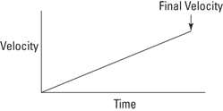
The average velocity is half the final velocity, and you know this because there’s constant acceleration. Your final velocity is vf = at, so your average velocity is half this:

So far, so good. Now you can plug this average velocity into the equation and get

And this becomes

You can also put in tf – ti rather than just plain t:

Congrats! You’ve worked out one of the most important equations you need to know when you work with physics problems relating acceleration, displacement, time, and velocity.

Notice that when you derived this equation, you had an initial velocity of zero. What if you don’t start off at zero velocity, but you still want to relate acceleration, time, and displacement? What if you’re initially going 100 miles per hour? That initial velocity would certainly add to the final distance you go. Because distance equals speed multiplied by time, the equation looks like this (don’t forget that this assumes the acceleration is constant):

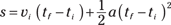
You also see this written simply as the following (where t stands for Δt, the time over which the acceleration happened):

Calculating acceleration and distance

With the formula relating distance, acceleration, and time, you can find any of those values, given the other two. If you have an initial velocity, too, finding distance or acceleration isn’t any harder. In this section, I work through some physics problems to show you how these formulas work.

Finding acceleration

Given distance and time, you can find acceleration. Say you become a drag racer in order to analyze your acceleration down the dragway. After a test race, you know the distance you went — 402 meters, or about 0.25 miles (the magnitude of your displacement) — and you know the time it took — 5.5 seconds. So what was your acceleration as you blasted down the track?

Well, you know how to relate displacement, acceleration, and time (see the preceding section), and that’s what you want — you always work the algebra so that you end up relating all the quantities you know to the one quantity you don’t know. In this case, you have

(Keep in mind that in this case, your initial velocity is 0 — you’re not allowed to take a running start at the drag race!) You can rearrange this equation with a little algebra to solve for acceleration; just divide both sides by t2 and multiply by 2 to get

Great. Plugging in the numbers, you get the following:

Okay, the acceleration is approximately 27 meters per second2. What’s that in more understandable terms? The acceleration due to gravity, g, is — 9.8 meters per second2, so this is about 2.7 g’s — you’d feel yourself pushed back into your seat with a force about 2.7 times your own weight.

Figuring out time and distance

Given a constant acceleration and the change in velocity, you can figure out both time and distance. For instance, imagine you’re a drag racer. Your acceleration is 26.6 meters per second2, and your final speed is 146.3 meters per second. Now find the total distance traveled. Got you, huh? “Not at all,” you say, supremely confident. “Just let me get my calculator.”

You know the acceleration and the final speed, and you want to know the total distance required to get to that speed. This problem looks like a puzzler because the equations in this chapter have involved time up to this point. But if you need the time, you can always solve for it. You know the final speed, vf, and the initial speed, vi (which is zero), and you know the acceleration, a. Because vf – vi = at, you know that

Now you have the time. You still need the distance, and you can get it this way:

The second term drops out because vi = 0, so all you have to do is plug in the numbers:

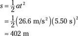
In other words, the total distance traveled is 402 meters, or a quarter mile. Must be a quarter-mile racetrack.

Finding distance with initial velocity

Given initial velocity, time, and acceleration, you can find displacement. Here’s an example: There you are, the Tour de France hero, ready to give a demonstration of your bicycling skills. There will be a time trial of 8.0 seconds. Your initial speed is 6.0 meters/second, and when the whistle blows, you accelerate at 2.0 m/s2 for the 8.0 seconds allowed. At the end of the time trial, how far will you have traveled?

You could use the relation s = (1/2)at2, except you don’t start off from zero speed — you’re already moving, so you should use the following:

In this case, a = 2.0 m/s2, t = 8.0 s, and vi = 6.0 m/s, so you get the following:

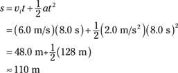
You write the answer to two significant digits — 110 meters — because you know the time only to two significant digits (see Chapter 2 for info on rounding). In other words, you ride to victory in about 110 meters in 8.0 seconds. The crowd roars.

Linking Velocity, Acceleration, and Displacement

Say you want to relate displacement, acceleration, and velocity without having to know the time. Here’s how it works. First, you solve the acceleration formula for the time:

Because displacement is and average velocity is when the acceleration is constant, you can get the following equation:

Substituting for the time, t, you get

After doing the algebra and simplifying, you get

Moving the 2a to the other side of the equation, you get an important equation of motion:

vf2 – vi2 = 2as

Whew. If you can memorize this one, you can relate velocity, acceleration, and displacement. Put this equation to work — you see it often in physics problems.

Finding acceleration

There you are, getting into your Physics racer as the crowd cheers. It’s time for some hefty acceleration. You get out your clipboard. What acceleration would you need to end up at 100 miles per hour at the end of a 1.0-mile racetrack?

Okay, you think. You need an equation that relates speed, acceleration, and displacement. It’s time for

vf2 – vi2 = 2as

In this case, it’s even a little easier, because you know that the initial velocity is 0 (vi = 0), so you have

vf2 = 2as

Well, well, it looks like the problem is half-solved. Putting in the numbers gives you

(100 mph)2 = 2a(1.0 mile)

Now solve for a:

Miles per hour2? What the heck kind of units are those? Change that to something more understandable, such as mph per second. To change one of the per-hour units to per-second, multiply by the conversion factor (see Chapter 2):

So your velocity would be increasing by only 1.4 mph every second — that’s not too outrageous — you’d feel a mild acceleration, that’s all.

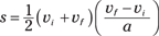
Solving for displacement

Now say that you’re at the end of the first mile and want to see how far you’d have to go — at the same acceleration — to get to 200 miles per hour. Once again, you need to relate velocity, acceleration, and displacement, so this equation is your baby:

vf2 = 2as

Here, you want to solve for s, the displacement, and you get this:

Great. Now for some numbers. In this case, vf = 200 mph, vi = 100 mph, and a = 5,000 miles/hour2, and you don’t know s at this point. To find s, plug your numbers into the equation you found for s to get

So it would take 3.0 additional miles to get you up to 200 mph.

Finding final velocity

Here’s one more example. Say you’re in your rocket ship, happily speeding along at some 3.25 kilometers per second (about 7,280 miles per hour) when you see a sign: Speed Zone 215 km Ahead — New Speed Limit: 3.0 km/s.

You jam on the brakes (which are a retro rocket in the front of the rocket ship). The retro rocket is capable of accelerating your ship at –10.0 meters/second2.

It’s a tense moment. Will you get your speed down to below 3.0 kilometers per second in 215 kilometers of acceleration? Find out, using your old friend:

vf2 – vi2 = 2as

In this case, you want to solve for the final speed, which is

vf2 = 2as + vi2

where a = –10.0 m/s2, s = 215 km = 215,000 m, and vi = 3.25 km/s = 3,250 m/s. Plugging in the data and solving for vf gives you the following:

Whew, you think — 2.50 kilometers per second is well under the speed limit of 3.0 kilometes per second. You’re safe.

You can now consider yourself a motion master.