Chapter 13

Springs ’n’ Things: Simple Harmonic Motion

In This Chapter

Understanding force when you stretch or compress springs

Going over the basics of simple harmonic motion

Mustering up the energy for simple harmonic motion

Predicting a pendulum’s motion and period

In this chapter, I shake things up with a new kind of motion: periodic motion, which occurs when objects are bouncing around on springs or bungee cords or are swooping on the end of a pendulum. This chapter is all about describing their motion. Not only can you describe their motion in detail, but you can also predict how much energy bunched-up springs have, how long a pendulum will take to swing back and forth, and more.

Bouncing Back with Hooke’s Law

Objects that can stretch but return to their original shapes are called elastic. Elasticity is a valuable property, because it allows you to use objects such as springs for all kinds of applications: as shock absorbers in lunar landing modules, as timekeepers in clocks and watches, and even as hammers of justice in mousetraps.

In this section, I introduce Hooke’s law, which relates forces to how much a spring is stretched or compressed.

Stretching and compressing springs

Robert Hooke, a physicist from England, undertook the study of elastic materials in the 1600s. He discovered a new law, not surprisingly called Hooke’s law, which states that stretching or compressing an elastic material requires a force that’s directly proportional to the amount of stretching or compressing you do. For example, to stretch a spring a distance x, you need to apply a force that’s directly proportional to x:

Fa = kx

Here, Fa and x are the components of the applied force and displacement along the direction of the spring, such that

Positive values correspond to stretching

Negative values correspond to compression

The constant k is called the spring constant, and its units are newtons per meter (N/m).

Pushing or pulling back: The spring’s restoring force

In accordance with Newton’s third law, if an object applies a force to a spring, then the spring applies an equal and opposite force to the object. Hooke’s law gives the force a spring exerts on an object attached to it with the following equation:

F = –kx

where the minus sign shows that this force is in the opposite direction of the force that’s stretching or compressing the spring (see the preceding section for info on forces on springs).

The force exerted by a spring is called a restoring force; it always acts to restore the spring toward equilibrium. In Hooke’s law, the negative sign on the spring’s force means that the force exerted by the spring opposes the spring’s displacement.

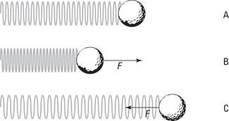
Figure 13-1 shows a ball attached to a spring. You can see that if the spring isn’t stretched or compressed, it exerts no force on the ball. If you push the spring, however, it pushes back, and if you pull the spring, it pulls back.

Hooke’s law is valid as long as the elastic material you’re dealing with stays elastic — that is, it stays within its elastic limit. If you pull a spring too far, it loses its stretchy ability. As long as a spring stays within its elastic limit, you can say that F = –kx. When a spring stays within its elastic limit and obeys Hooke’s law, the spring is called an ideal spring.

Figure 13-1: The direction of force exerted by a spring.

Suppose that a group of car designers knocks on your door and asks whether you can help design a suspension system. “Sure,” you say. They inform you that the car will have a mass of 1,000 kilograms, and you have four shock absorbers, each 0.5 meters long, to work with. How strong do the springs have to be? Assuming these shock absorbers use springs, each one has to support a mass of at least 250 kilograms, which weighs the following:

F = mg = (250 kg)(9.8 m/s2) = 2,450 N

where F equals force, m equals the mass of the object, and g equals the acceleration due to gravity, 9.8 meters per second2. The spring in the shock absorber will, at a minimum, have to give you 2,450 newtons of force at the maximum compression of 0.5 meters. What does this mean the spring constant should be? Hooke’s law says

F = –kx

Looking only at the magnitudes and therefore omitting the negative sign (look for its return in the following section), you get

Time to plug in the numbers:

The springs used in the shock absorbers must have spring constants of at least 4,900 newtons per meter. The car designers rush out, ecstatic, but you call after them, “Don’t forget, you need to at least double that if you actually want your car to be able to handle potholes.”

Getting Around to Simple Harmonic Motion

An oscillatory motion is one that undergoes repeated cycles. When the net force acting on an object is elastic, the object undergoes a simple oscillatory motion called simple harmonic motion. The force that tries to restore the object to its resting position is proportional to the displacement of the object. In other words, it obeys Hooke’s law.

Elastic forces suggest that the motion will just keep repeating (that isn’t really true, however; even objects on springs quiet down after a while as friction and heat loss in the spring take their toll). This section delves into simple harmonic motion and shows you how it relates to circular motion. Here, you graph motion with the sine wave and explore familiar concepts such as position, velocity, and acceleration.

Around equilibrium: Examining horizontal and vertical springs

Take a look at the golf ball in Figure 13-1. The ball is attached to a spring on a frictionless horizontal surface. Say that you push the ball, compressing the spring, and then you let go; the ball shoots out, stretching the spring. After the stretch, the spring pulls back and once again passes the equilibrium point (where no force acts on the ball), shooting backward past it. This happens because the ball has inertia (see Chapter 5), and when the ball is moving, bringing it to a stop takes some force. Here are the various stages the ball goes through, matching the letters in Figure 13-1 (and assuming no friction):

Point A: The ball is at equilibrium, and no force is acting on it. This point, where the spring isn’t stretched or compressed, is called the equilibrium point.

Point B: The ball pushes against the spring, and the spring retaliates with force F opposing that pushing.

Point C: The spring releases, and the ball springs to an equal distance on the other side of the equilibrium point. At this point, the ball isn’t moving, but a force acts on it, F, so it starts going back the other direction.

The ball passes through the equilibrium point on its way back to Point B. At the equilibrium point, the spring doesn’t exert any force on the ball, but the ball is traveling at its maximum speed. Here’s what happens when the golf ball bounces back and forth; you push the ball to Point B, and it goes through Point A, moves to Point C, shoots back to A, moves to B, and so on: B-A-C-A-B-A-C-A, and so on. Point A is the equilibrium point, and both Points B and C are equidistant from Point A.

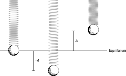
What if the ball were to hang in the air on the end of a spring, as Figure 13-2 shows? In this case, the ball oscillates up and down. Like the ball on a surface in Figure 13-1, the ball hanging on the end of a spring oscillates around the equilibrium position; this time, however, the equilibrium position isn’t the point where the spring isn’t stretched.

The equilibrium position is defined as the position at which no net force acts on the ball. In other words, the equilibrium position is the point where the ball can simply sit at rest. When the spring is vertical, the weight of the ball downward matches the pull of the spring upward. If the x position of the ball corresponds to the equilibrium point, xi, the weight of the ball, mg, must match the force exerted by the spring. Because F = kxi, you can write the following:

mg = kxi

Figure 13-2: A ball on a spring, influenced by gravity.

Solving for xi gives you the distance the spring stretches because of the ball’s weight:

When you pull the ball down or lift it up and then let go, it oscillates around the equilibrium position, as Figure 13-2 shows. If the spring is elastic, the ball undergoes simple harmonic motion vertically around the equilibrium position; the ball goes up a distance A and down a distance –A around that position (in real life, the ball would eventually come to rest at the equilibrium position, because a frictional force would dampen this motion).

The distance A, or how high the object springs up, is an important one when describing simple harmonic motion; it’s called the amplitude. The amplitude is simply the maximum extent of the oscillation, or the size of the oscillation.

Catching the wave: A sine of simple harmonic motion

Calculating simple harmonic motion can require time and patience when you have to figure out how the motion of an object changes over time. Imagine that one day you come up with a brilliant idea for an experimental apparatus. You decide to shine a spotlight on a ball bouncing on a spring, casting a shadow on a moving piece of photographic film. Because the film is moving, you get a record of the ball’s motion as time goes on. You turn the apparatus on and let it do its thing. See the results in Figure 13-3.

Figure 13-3: Tracking a ball’s simple harmonic motion over time.

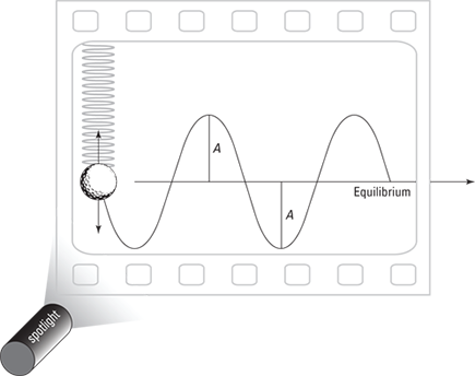
The ball oscillates around the equilibrium position, up and down, reaching amplitude A at its lowest and highest points. But take a look at the ball’s track: You can tell where the ball is moving fastest because that’s where the curve has the steepest slope. The ball goes fastest near the equilibrium point because of the acceleration caused by the spring force, which has been applied since the turning point. At the top and bottom, the ball is subject to plenty of force, so it slows down and reverses its motion.

The track of the ball is best modeled with a sine wave, which means that its track is a sine wave of amplitude A. (Note: You can also use a cosine wave, because the shape is the same. The only difference is that when a sine wave is at its peak, the cosine wave is at zero, and vice versa.)

You can get a clear picture of the sine wave if you plot the sine function on an xy graph like this:

y = sin x

In the rest of this section, I show you how the sine wave relates circular motion to simple harmonic motion.

Understanding sine waves with a reference circle

Take a look at the sine wave in a circular way. If you attach a ball to a rotating disk (see Figure 13-4) and you shine a spotlight on it, you get the same result as when you have the ball hanging from the spring (Figure 13-3): a sine wave.

The rotating disk, which you can see in Figure 13-5, is often called a reference circle. You can see how the vertical component of circular motion relates to the sinusoidal (sine-like) wave of simple harmonic motion. Reference circles can tell you a lot about simple harmonic motion.

As the disk turns, the angle, θ, increases in time. What does the track of the ball look like as the film moves to the right? Using a little trig, you can resolve the ball’s motion along the y-axis; all you need is the vertical (y) component of the ball’s position. At any one time, the ball’s y position is the following:

y = A sin θ

The vertical displacement varies from positive A to negative A in amplitude. In fact, you can say that you already know how θ is going to change in time because θ = ωt, where ω is the single component of the angular velocity — that is, the angular velocity along the axis of rotation of the disk — and t is time:

y = A sin(ωt)

You can now explain the track of the ball as time goes on, given that the disk is rotating with angular velocity ω.

Figure 13-4: The vertical component of the displacement of an object moving in a circle follows a sine wave.

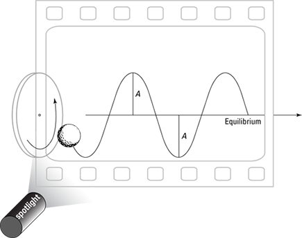
Figure 13-5: A reference circle helps you analyze simple harmonic motion.

Getting periodic

Each time an object moves around a full circle, it completes a cycle. The time the object takes to complete the cycle is called the period, and it’s generally measured in seconds. The letter used for period is T.

Look at Figure 13-5 in terms of the y motion on the film. During one cycle, the ball moves from y = A to –A and then back to A. When the ball goes from any point on the sine wave and passes through one whole wave (including one peak and one trough) back to the next equivalent point on the sine wave later in time, it completes a cycle. The time the ball takes to move from a certain position back to that same position while moving in the same direction is its period.

How can you relate the period to something more familiar? When an object moves in a full circle, completing a cycle, the object goes 2π radians. It travels that many radians in T seconds, so its angular speed, ω (see Chapter 11), is

Multiplying both sides by T and dividing by ω allows you to solve for the period. Now you can relate the period and the angular speed:

Sometimes you speak in terms of the frequency of periodic motion, not the period. The frequency is the number of cycles that are completed per second.

For instance, if the disk from Figure 13-4 rotates at 1,000 full turns per second, the frequency, f, would be 1,000 cycles per second. Cycles per second are also called hertz, abbreviated Hz, so this frequency would be 1,000 hertz.

So how do you connect frequency, f, to period, T? T is the amount of time one cycle takes, so here’s how you can define frequency:

Because ω = 2π/T and Tf = 1, you can rewrite the angular-velocity equation in terms of frequency:

In simple harmonic motion, the angular velocity, ω, is often referred to as angular frequency. Don’t confuse the wave’s frequency, f, with the angular frequency.

Remembering not to speed away without the velocity

Take a look at Figure 13-5, where a ball is rotating on a disk. In the section “Understanding sine waves with a reference circle,” earlier in this chapter, you figure out that

y = A sin(ωt)

where y stands for the y coordinate and A stands for the amplitude of the motion. At any point y, the ball also has a certain velocity, which varies in time also. So how can you describe the velocity mathematically? Well, you can relate tangential velocity to angular velocity like this (see Chapter 11):

v = rω

where r represents the radius. Because the radius of the circle is equal to the amplitude of wave it corresponds to, r = A. Therefore, you get the following equation:

v = Aω

Does this equation get you anywhere? Sure, because the ball’s shadow on the film gives you simple harmonic motion. The velocity vector (see Chapter 4) always points tangential to the circle — perpendicular to the radius — so you get the following for the y component of the velocity at any one time:

vy = Aω cos θ

And because the ball is on a rotating disk, you know that θ = ωt, so

vy = Aω cos(ωt)

This equation describes the velocity of any object in simple harmonic motion. Note that the velocity changes in time — from –Aω to 0 and then to Aω and back again to 0. So the maximum velocity, which happens at the equilibrium point, has a magnitude of Aω. Among other things, this equation says that, for a given angular velocity, the maximum velocity (v) is directly proportional to the amplitude (A) of the motion: Simple harmonic motion of greater amplitude has a larger maximum velocity, and vice versa.

For example, say that you’re on a physics expedition watching a daredevil team do some bungee jumping. You notice that the team members are starting by finding the equilibrium point of their new bungee cords when a jumper is dangling from it but not bouncing, so you measure that point.

The team decides to release their leader from a few meters above the equilibrium point, and you watch as he flashes past the point and then bounces back at a speed of 4.0 meters per second at the equilibrium point. Ignoring all caution, the team lifts its leader to a distance 10 times greater away from the equilibrium point and lets go again. This time you hear a distant scream as the costumed figure hurtles up and down. What’s his maximum speed?

You know that, on the first run, he was going 4.0 meters per second at the equilibrium point, the point where he achieved maximum speed; you know that he started with an amplitude 10 times greater on the second try; and you know that the maximum velocity is proportional to the amplitude. Therefore, assuming that the frequency of his bounce is the same, he’ll be going 40.0 meters per second at the equilibrium point — pretty speedy.

Including the acceleration

You can find the displacement of an object undergoing simple harmonic motion with the equation y = A sin(ωt), and you can find the object’s velocity with the equation v = Aω cos(ωt). But you have another factor to account for when describing an object in simple harmonic motion: its acceleration at any particular point. How do you figure it out? No sweat. When an object is going around in a circle, the acceleration is the centripetal acceleration (see Chapter 11), which is

a = rω2

where r is the radius and ω is the single component of angular velocity (that is, the angular velocity in the direction of the [constant] axis of rotation). And because r = A — the amplitude — you get the following equation:

a = Aω2

This equation represents the relationship between centripetal acceleration, a, and angular velocity, ω. To go from a reference circle (see the earlier section “Understanding sine waves with a reference circle”) to simple harmonic motion, you take the component of the acceleration in one dimension — the y direction here — which looks like this:

a = –Aω2 sin θ

The negative sign indicates that the y component of the acceleration is always directed opposite the displacement (the ball always accelerates toward the equilibrium point). And because θ = ωt, where t represents time, you get the following equation for acceleration:

a = –Aω2 sin(ωt)

Now you have the equation to find the acceleration of an object at any point while it’s moving in simple harmonic motion.

For example, say that your phone rings, and you pick it up. You hear “Hello?” from the earpiece.

“Hmm,” you think. “I wonder what the maximum acceleration of the diaphragm in the phone is.” The diaphragm (a metal disk that acts like an eardrum) in your phone undergoes a motion very similar to simple harmonic motion, so calculating its acceleration isn’t any problem. Measuring carefully, you note that the amplitude of the diaphragm’s motion is about 1.0 × 10–4 meters. So far, so good. Human speech is in the 1.0-kilohertz (1,000 hertz) frequency range, so you have the frequency, ω. And you know that the maximum acceleration equals the following:

amax = Aω2

Also, ω = 2πf, where f represents frequency. Replace ω with 2πf, and you can plug in the amplitude and frequency to find your answer:

amax = A(2πf)2 = (1.0 × 10–4 m)[2π(1,000/s)]2 ≈ 3,940 m/s2

You get a value of 3,940 meters per second2. That seems like a large acceleration, and indeed it is; it’s about 402 times the magnitude of the acceleration due to gravity! “Wow,” you say. “That’s an incredible acceleration to pack into such a small piece of hardware.”

“What?” says the impatient person on the phone. “Are you doing physics again?”

Finding the angular frequency of a mass on a spring

If you take the information you know about Hooke’s law for springs (see the earlier section “Bouncing Back with Hooke’s Law”) and apply it to what you know about simple harmonic motion (see “Getting Around to Simple Harmonic Motion”), you can find the angular frequencies of masses on springs, along with the frequencies and periods of oscillations. And because you can relate angular frequency and the masses on springs, you can find the displacement, velocity, and acceleration of the masses.

Hooke’s law says that

F = –kx

where F is the force exerted by the string, k is the spring constant, and x is displacement from equilibrium. Because of Isaac Newton (see Chapter 5), you know that force also equals mass times acceleration:

F = ma

These force equations are in terms of displacement and acceleration, which you see in simple harmonic motion in the following forms (see the preceding section):

x = A sin(ωt)

a = –Aω2 sin(ωt)

Inserting these two equations into the force equations gives you the following:

ma = –kx

m[–Aω2 sin(ωt)] = –kA sin(ωt)

Divide both sides by –A sin(ωt), and this equation breaks down to

mω2 = k

Rearranging to put ω on one side of the equation gives you the formula for angular frequency:

You can now find the angular frequency (angular velocity) of a mass on a spring, as it relates to the spring constant and the mass. You can also tie the angular frequency to the frequency and period of oscillation (see “Getting periodic”) by using the following equation:

With this equation and the earlier angular-frequency formula, you can write the formulas for frequency and period in terms of k and m:

Say that the spring in Figure 13-1 has a spring constant, k, of 15 newtons per meter and that you attach a 45-gram ball to the spring. What’s the period of oscillation? After you convert from grams to kilograms, all you have to do is plug in the numbers:

The period of the oscillation is 0.34 seconds. How many bounces will you get per second? The number of bounces represents the frequency, which you find this way:

You get nearly 3 oscillations per second.

Because you can relate the angular frequency, ω, to the spring constant and the mass on the end of the spring, you can predict the displacement, velocity, and acceleration of the mass, using the following equations for simple harmonic motion (see the section “Catching the wave: A sine of simple harmonic motion” earlier in this chapter):

y = A sin(ωt)

v = Aω cos(ωt)

a = –Aω2 sin(ωt)

Using the example of the spring in Figure 13-1 — with a spring constant of 15 newtons per meter and a 45-gram ball attached — you know that the angular frequency is the following:

You may like to check how the units work out. Remember that 1 N = 1 kg·m/s2, so the units you get from the preceding equation for the angular velocity work out to be

Say, for example, that you pull the ball 10.0 centimeters before releasing it (making the amplitude 10.0 centimeters). In this case, you find that

x = (0.10 m) sin[(18 s–1)t]

v = (0.10 m)(18 s–1) sin[(18 s–1)t]

a = –(0.10 m)(18 s–1)2 cos[(18 s–1)t]

Factoring Energy into Simple Harmonic Motion

Along with the actual motion that takes place in simple harmonic motion, you can examine the energy involved. For example, how much energy is stored in a spring when you compress or stretch it? The work you do compressing or stretching the spring must go into the energy stored in the spring. That energy is called elastic potential energy and is equal to the force, F, times the distance, s:

W = Fs

As you stretch or compress a spring, the force varies, but it varies in a linear way (because in Hooke’s law, force is proportional to the displacement). Therefore, you can write the equation in terms of the average force, :

The distance (or displacement), s, is just the difference in position, xf – xi, and the average force is (1/2)(Ff + Fi). Therefore, you can rewrite the equation as follows:

Hooke’s law says that F = –kx. Therefore, you can substitute –kxf and –kxi for Ff and Fi:

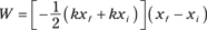
Distributing and simplifying the equation gives you the equation for work in terms of the spring constant and position:

The work done on the spring changes the potential energy stored in the spring. Here’s how you give that potential energy, or the elastic potential energy:

For example, suppose a spring is elastic and has a spring constant, k, of 1.0 × 10–2 newtons per meter, and you compress the spring by 10.0 centimeters. You store the following amount of energy in it:

You can also note that when you let the spring go with a mass on the end of it, the mechanical energy (the sum of potential and kinetic energy) is conserved:

PE1 + KE1 = PE2 + KE2

When you compress the spring 10.0 centimeters, you know that you have 5.0 × 10–5 joules of energy stored up. When the moving mass reaches the equilibrium point and no force from the spring is acting on the mass, you have maximum velocity and therefore maximum kinetic energy — at that point, the kinetic energy is 5.0 × 10–5 joules, by the conservation of mechanical energy (see Chapter 9 for more on this topic).

Swinging with Pendulums

Other objects besides springs, such as pendulums, move in simple harmonic motion. In Figure 13-6, a ball tied to a string swings back and forth.

Figure 13-6: A pendulum moves in simple harmonic motion.

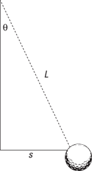
The torque, τ, that comes from gravity is the weight of the ball (which is a force of magnitude mg directed downward — hence the minus sign) multiplied by the lever arm, s (for more on lever arms and torque, see Chapter 11):

τ = –mgs

Here’s where you make an approximation. For small angles θ, the distance s approximately equals Lθ, where L is the length of the pendulum string:

τ = –mgLθ

This equation resembles Hooke’s law, F = –kx, if you treat mgL as you would a spring constant. In Chapter 12, I show you the relation between torque and angular acceleration, and you see that the angular variables obey the same equations as their linear equivalents. Therefore, the calculation goes in just the same way as for the spring. In the angular variables:

Στ = Iα

Just as in the case of the spring, the pendulum undergoes simple harmonic motion, with

θ = A sin(ωt)

α = –Aω2 sin(ωt)

Plug in the torque of the pendulum and the values of α and θ to get

Iα = –mgLθ

I[–Aω2 sin(ωt)] = –mgLA sin(ωt)

Then solve for ω to get this:

The moment of inertia equals mr2 for a point mass (see Chapter 12), which you can use here, assuming that the ball is small compared to the pendulum string. For the pendulum, the radius r is the length of the string, L. This gives you the following equation:

Now you can plug this angular velocity into the equations for simple harmonic motion. You can also find the period of a pendulum with the following equation:

where T represents period. If you substitute the preceding form for ω, you get this:

Then rearrange to find the period:

Note that this period is actually independent of the mass on the pendulum!