During recent decades, probability theory models for mathematical simulations (particularly that of Monte Carlo (MC)) have developed intensely. The domains for studying safety coefficients have become disadvantageous. In the last two decades, more than 3,000 published articles [RUB 81] have dealt with variable simulation using the Monte Carlo (MC) method. With the help of informatics, the use of this often time consuming method, in terms of calculation time, was encouraged. The first applications of the MC method were carried out on the analysis results of Stefan–Boltzmann’s equation. In 1908, the statistician student was already using this method to estimate the correlation of coefficients using his famous test of Student’s law. We will now clarify some of the terminology that characterizes simulation methods.
The method, contrary to popular belief, does not come from a person named Monte Carlo, but instead from the name of the town Monte Carlo, in the principality of Monaco (mid-France). It was not von Neumann who invented it, but instead von Neumann and Ulam [NEU 51] who introduced the concept, during the Second World War. The motif was not linked to gambling games from the Monte Carlo casinos. It was instead a secret war code from an American scientific work which was preparing for the atomic bomb in Los Alamos (USA). The problem lay in using the method to simulate random variables relating to material behavior (neutrons), leading to diffusion with difficulty. During that period (without the current power of computers), the complex and multidimensional evaluation of integrals led researchers to resolve integral equations by means of an analytical solution, using the so-called MC method. It would now seem restrictive to believe that this method only applies to purely random phenomena. It is also used in stochastic solutions to rational deterministic problems.
The simulation of variable analysis was defined as an efficient technique to analyze the experiences of singular or structural models. The true definition, according to R.Y. Rubenstein [RUB 81], is not often completely linked to the MC method. When we integrate random variables, apart from their statistical law distributions, we can precisely see MC simulation. Consider that random variables are independent (in our case a0 and m), and uniformly distributed on the interval [0, 1]. The generation of random numbers between 0 and 9 is approximated with equal probability.
We indicate here the academic (yet largely simple) confusion surrounding the method: the simulation of analyzed variables, whether correlated or not, is not always an MC simulation. It may be a simple combination of variables, certainly similar to the MC method, but not quite the method itself. For example, to simulate random variables which are differently distributed and not correlated, a random average run can be carried out or indeed the Kolmogorov–Smimov method can be conducted to qualify the number of runs. This is an MC simulation method of random variables.
Numerous authors [SCH 85, SCH 87, FOG 82] have worked on MC simulation. Of course, not all used the same procedures but the final interpretation was often the same. We believe that this is essentially due to the calculation time that each author attempted to reduce. The problem of convergence of stability and failure probability is omnipresent. This can seriously jeopardize a simulation of the MC type.
The essential problem lies in studying how the safety (stability) of constructions is affected by the alteration of unfamiliar conditions (which are likely to intervene) when these conditions depart from the norm. The variables which characterize these various elements have a random character. We can therefore state that safety is a function of random variables and its study should be carried out by probabilities. If a structure is made with the purpose of being very unlikely to “fail”, it is necessary to know the abnormal factors which it is exposed to, before we can decide on a degree of safety (or of failure).
Constructions, in general, and welded structures, in particular, are designed with the aim of responding to various needs with the implicit understanding of a certain level of safety or probable failure. Given that the probability which guarantees failure, i.e. the probability that a structure reaches failure level, is not a physically palpable entity, it is instead mathematically estimated based on physical and/or unknown data. We could say that this probability is “justifiably” calculated, as it rests on the large assurance of reputed safety [FRE 47, FRE 66].
In the case studies outlined in this work, we suppose that the parameters of resistance (R), stress (S), geometry g(a/T), coefficients (ρ, θ) respective to local geometrical correction (taking into account the radius and angle of the joint at the foot of the welding band) and intrinsic material coefficients (C, m) are all correctly estimated. Yet they are nearly all variable, added to the issue of random external factors such as wind, waves, corrosion, fatigue, etc.
There are many codes and rules [CSA 81, CSA 11, LIN 73, CIR 77, 81, AME 87, API 87, SIG 67, HOH 84, DIT 79, DIT 86a, DIT86b, GRO 98, AME 84, DNV 82, CIR 81] which suggest to the user the limits to which they are authorized to consider proportional hypotheses to ensure sufficient construction safety. Nowadays, modern rules use the best knowledge that the designer could possibly have in the dynamics of materials. Sometimes we can see the so-called safety coefficients used in a purely academic way. This is a great danger when we consider that it is not only materials which evolve and develop, but also their dynamics. How then can we trust a Young’s coefficient or an admissible stress selected from a manual?
As serious as it is, the recommended manual [COR 69, COR 67, CIR 81] remains erroneous in the values that it proposes if it is not continually updated. As an example, the Canadian and European rules for metallic construction suppose that the probabilities of reaching a limit state are 10–5 in limit state, and 5 × 10⁻⁵ in service limit state.
As we have already mentioned, cross-joined structures have a limit state of fatigue that fracture mechanics takes into account, through the Paris–Erdogan law. These structures are often governed by a very rigorous design, especially at the foot of the welding band. The causes of uncertainty are often linked to physical phenomena: hydrodynamic loads, particularly aggressive environments, stress intensity factors, tenacity, empiricism of behavior laws, etc. Fatigue cracking in metals is a multidisciplinary phenomenon which remains the object of many scientific debates [SIG 67]. Fatigue cracking often leads to unknown mechanical structures being analyzed using probabilistic theories with multiple correlations developed by Markov’s chain theory, among others.
Faced with convergence problems, some authors such as Hohenbichler [HOH 84] have preferred to settle on a linear approximation of the limit state surface near the “design point”. This calculation is carried out beforehand by optimizing the area of true failure or on a quadratic approximation of this area.
For example, a linear approximation of the limit state surface provides the huge advantage of allowing a numerical integration of probability densities in the area of failure. It is entirely sufficient with regard to the highly possible distortion on the true surface. This surface is of course strengthened by the hyperplane surface. The results from level II are sometimes similar to those arising from level III [SEL 93]. Long before the 1990s, an interesting study carried out by Schuëller et al. [SCH 79] dealt with this issue. It is well worth consulting.
With calculation systems, the inherent risks to engineering science essentially result from what we do not know with sufficient accuracy. Intuition plays a large part in the field of reliability [PRO 87]. When in doubt, “you cannot doubt badly”. The data relevant to projects involve materials, their geometric dimensions, and their diverse faculties of “aging”. Many physical parameters are marked with uncertainty, leading to their random and unknown character. We cannot calculate with certainty what has already existed. Starting new design projects can also lead toward mitigation, and even the opposite of the expected development of parameters which constitute the mathematical skeleton of models.
The project becomes less disadvantageous when we consider a hypothesis where sufficient information is collected to establish a quantitative estimation of risk. Statistical tools rationalize the measuring of uncertainties to try and make structures reliable. We will limit ourselves here to just present the necessary statistical tools for the probabilistic approach in the domain of dimensional metrology. Their use aims to estimate parameters of probability laws, which have been chosen a priori and/or on the basis of conformity tests.
To emphasize this point, the statistical approach, in many other areas (science and equipment in medicine), is very risky and even hazardous. One simple way to properly understand the effect of unknown uncertainties affecting material and structural behavior is to place them in conditions where they are subjected to simulated uncertainties. It is then possible to estimate mathematical expectations and the variance in variables necessary for the understanding of many phenomena (stresses, resistances, displacement, safety margins). We can also treat simulated samples as a group of observations and apply an appropriate statistical treatment to them. The making of the atomic bomb (at Los Alamos, USA) is an example of the use of the MC simulation method. The principle of MC simulations is to generate a group of pseudo-random realizations from a random variable or random field. To obtain a realization x from the variable X obtained from the distribution function PX(·), we simulate a number z uniformly distributed on [0,1], and then apply a formula of the following type:
[7.1]
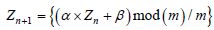
Many simulation algorithms on a uniformly distributed number [0,1] are based on linear congruence, as follows:
In this congruence relationship, it is necessary to define an initial value z0 of Z. The quality of generation is linked to the period of return for the same realizations of Z, as well as the dispersion of these realizations. The choice of α, β, and m depends on this quality. As an example, we can mention an effective choice arising from the literature such as the “Mersenne Twister” from Matsumoto and Nishimura:
In the present work, we have used the software MathCAD to generate a group of pseudo-random variables of a RV.
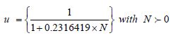
According to the Box and Muller method, if z1 and z2 are two numbers uniformly distributed on [0,1], the number u defined by  is a reduced centered Gaussian variable.
 we apply: x = u × σx + µx. we apply x = Exp (u × σLx + µLx) where µLx and
  are the average and the variance of ln(x).
In this case we can use the general relationship  . Note that for the majority of laws of exponential type (Weibull), the inversion of the distribution function does not create a problem. For other laws, a numeric inversion would often prove necessary (see beta law).
The vector X of correlated variables is characterized by its expected mathematical vector µx, its variance–covariance matrix Σx, and the group of marginal distribution functions PX1, …, PXn. The awareness of the latter is often more obvious than that of linked probability density.
Starting from the simulation of a vector U to independent reduced centered Gaussian components, we can build a construction of Gaussian X by:
Σx = [C] × [C]T, where [C] is an inferior triangular matrix, obtained by a Choleski transformation.
To do this, we must use the so-called Rosenblatt transformations. By simply knowing the marginal probability densities of X1 and X2, it is possible to express their linked density by the following relationship:
[7.4]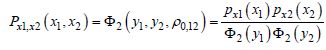
where:
Y1 and Y2 are two reduced centered Gaussian variables with the so-called fictitious correlation ρ0,12;
Φ2(·) is the reduced centered binominal density.
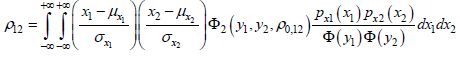
With the correlation ρ12 already known between X1 and X2, the following relation is expressed as:
This is a relationship from which we can extract the fictitious correlation value ρ0,12. In the literature, some approximate expressions of ρ0,12 have been proposed by Professor Der Kiureghian and Liu [KIU 85, LIU 86, LIU 91] for different marginal probability laws. These suggestions are subject to restrictions on coefficients of variations of variables X1 and X2 and on the value range of their correlation, according to marginal laws.
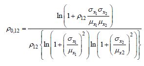
For example, note that for two log-normal variables, ρ0,12 is expressed exactly as follows:
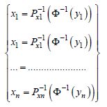
The simulation procedure of an X construction therefore consists of determining the fictitious covariance matrix Σy and then simulating Y by x = [c] × u + µx with µy = 0 to finally end up at x1,...,xn by the following:
In the present work, we limit ourselves to an MC simulation for basic applications arising from mechanical engineering techniques.
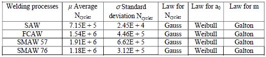
The considered variables in this chapter are random. They have been simulated [GRO 94] by their respective distribution laws, i.e. Weibull law for initial cracking (a0), log-normal (Galton) law for m-coefficients and normal (Gaussian) law for the number of cycles Ncycles.
Beforehand, it is considered that failure is possible. This eventuality is therefore more or less probable. The degree of failure will be characterized by the probability when the equality (R – S) < 0 is verified. Therefore, let this probability PF be expressed as:
where:
M is the safety margin;
PF is the probability of fracture (failure).
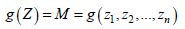
The model considered presents uncertainties which are essentially due to unknown factors brought about by initial cracking (a0) by material properties. It is vital to pay attention to the choice of conditions which risk being considered as a normal distribution. The limit state function g(z) as a mode of reliability is formulated in finite (n) terms. In general, one or more non-random base variables correspond to the limit state function presented by a safety margin M. This is defined by the following expression:
where Z represents (n) vectors of random base variables (a0 and m).
These random base variables can be dependent (or independent). The failure probability which results when M < 0 is represented by PF and is written as follows:
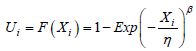
F(z) is the probability density function of (z1, z2, …, zn). This allows the reliability index to be calculated, with the help of the expression:
where Φ(·) is the function of the reduced centered random variable from normal law.
The relationship between the reliability index βc and the failure probability PF takes the graphical form as presented in Chapter 5. De Moivre’s law, reported by Laplace and then by Gauss (lending to the habitual name of Gaussian law or normal law), is largely utilized, which at times erroneously causes certain adequacy tests to be used in manipulations. The use of Gaussian law is often justified, if not indispensable, but in many problems fundamentally incorrect, if not absurd. It does not seem inappropriate here for us to comment on these observations of the abusive use of the normal law.
In our case study, we will be considering three distinct laws to simulate our parameters of cracking. The increment of (100 × a0) is made on the probability density function of Weibull law with two parameters. The m coefficient is also random and is chosen in the same way as the a0 but on a probability density function of Galton (log-normal) law.
After having read and calculated the parameters which will allow us to find the numbers of corresponding cycles and will integrate the simulated random variables a0 and m, we can then proceed to a mathematical statistical simulation of the results of Ni found by this classic variable simulation. Note that the random variables of the distribution function FN(n) are calculated as being close to 7.5 × 10⁻⁸.
We will also calculate the parameters a0 and m using the direct safety margin method with the help of the integral damage indicator. The safety margin calculation often arises when double integrals need to be calculated. To simplify this problem, we can employ the MC simulation method.
Designed by O. Ditlevsen and P. Bjerager [DIT 86] as the method of Gaussian safety margins, it is often used to resolve problems of mechanical reliability in structures and components. It is also used to design the geometrical configuration of Gaussian distributions. According to O. Ditlevsen [DIT 79, DIT 81], all structures can use a reliability application through boundary theory, especially when the system is redundant (and/or in a series). Sometimes, boundary theory can be hugely complex in terms of application.
The reliability index β can also be calculated using the Hasofer–Lind theory (βHL) [HAS 74], which is the smallest Euclidian distance from the origin of the failure surface (see Figure 5.2) in a reduced space of non-correlated, reduced, centered, normal variables. This is very relevant in our scenario of treating a0 and m a priori as two parameters from which we cannot presume a correlation. In the last instance, the MC simulation method does not require any particular remarks. It is, as a matter of course, the most appropriate reliability model for a singular structure [DIT 86]. Also, it is simple in terms of application. The advantages and disadvantages of the MC method are as follows.
Advantages:
Disadvantages:
In reality, the problem with this method rests with the “calculation time” factor and the complexity of the procedure generalization concern, for all types of structural problems, i.e. the capacity to treat multiple cases of reliability (aeronautic, maritime structures, buildings, and other industrial equipment). Numerous authors have analyzed and studied MC simulation techniques to try and free it from its inability to resolve problems with double integrals to attain failure probability. We class these methods into the following three types:
The results from the probabilistic treatment of a number of cycles from previous simulations of random variables allows us to see the importance of the engineering risk of fracture in the singular cross-joined structure. After having listed what we have just mentioned, we will attempt to show the efficiency of MC simulation in calculating the failure probability of a structure. Remember that the constant parameters of the behavior law are T, Δσ, acr, with the metal sheet thickness (25 mm), the nominal stress (150 MPa), and the critical crack (mm, arbitrarily fixed).
We can also remark that the random choice of these parameters is carried out on probability density functions which have already been plotted. We are choosing an increment of 10–5 which will allow us to sort the 10 randomly chosen values among the a0 and m of the respective probability density functions. The 100 chosen values among the a0 and m are grouped into the following table:
Table 7.1. Results of MC simulations on four welding processes
| Welding processa | a0_1st to a0_100th | m_1st to m_100th |
| SAW | 0.0027 to 0.0119 | 2.1821 to 3.3335 |
| FCAW | 0.0027 to 0.0180 | 2.1563 to 3.0648 |
| SMAW 57 | 0.0013 to 0.0134 | 2.5590 to 3.0580 |
| SMAW 76 | 0.0027 to 0.0196 | 2.4285 to 3.0392 |
aThe experiments were carried out by Professor T. Lassen (Norway). With his kind and generous permission we have recovered the data to conduct a thesis study [GRO 94, GRO 98].
To select an n number from the group {0, 1, 2, 3, 4, 5, 6, 7, 8, 8, 9} we set a rule for ourselves from the table of random numbers. For example, we choose the number in the left corner and then the number below each of the N first blocks, which gives N = 5, 5, 8, 1, 5. Other techniques permit a direct reading from the table of random numbers. In our case, the result is simple. For n = 5 × 5, an N at random will be 68645.
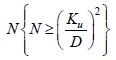
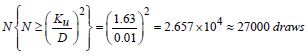
The problem studied here is simple and based on a necessary drawing from the Kolmogorov–Smirnov (KS) test. For example, by trying to limit the uncertainty to ± 1%, i.e. the uncertainty D = 0.01 on the simulation of probability density function, we choose a level of confidence 99.9%, i.e. α = 0.01 and we obtain N ≥ 2.657 × 10⁴ draws. Ku is a coefficient read in the following table:
Table 7.2. Determination of the number of necessary draws in MC SIM
Source: J. Cadiou [CAD 84] Techniques of the Engineer, pp. T-4 301–4.

The problem of drawing at random is variously realized. We have already mentioned the drawing technique based on the KS test. Having judged this test as being well adapted to our simulation variables, we will now apply it in this study. Now we will use the MC simulation of random variables from a Weibull law with two parameters. The random drawing process is carried out in the following stages:
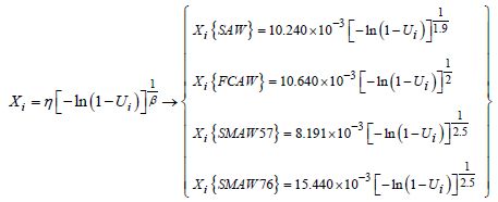
First stage: Obtain five random draws from the a0i in Weibull’s distribution of parameter β with scale η. Call Ui a random uniform number and we get the Weibull’s distribution of
In the Eularian law Γ (see table A.1. in the Appendix). We can recover the values of β and η, and thus for each joining process we will have Xi, a random steady variable:
We have used the software MathCAD for Ui = 100. The results are as follows:
Table 7.3. Results of statistical distribution functions for Ui = 100
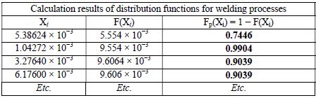
In this way we can steady the random variables Xi for the Weibull law with two parameters and thus calculate the distribution function and probability densities for each random draw, with the help of the Kolmogorov–Smirnov approach.
Second stage: The work set out in the first stage is resumed to calculate the number of cycles, relative to each of the four welding processes. We will thus carry out a statistical study to imitate the number of cycles found through the simulation of random variables a0 and m. Recall that the distribution laws for each random variable which intervene in probability failure density calculations all obey the following laws:
Table 7.4. Statistical distribution laws applied to the four welding processes [LAS 92, GRO 94]
| Distribution laws by welding processes | |
| Random variables Xi | Statistical law Fp(Xi) = 1 - F(Xi) |
| Initial cracks, a0 | Weibull law with two parameters |
| Paris coefficients, m | Log-normal law (Galton) |
| Number of cycles N | Normal law (Laplace-Gauss) |
We will now calculate the reduced, centered, normal law with an accuracy of (7.5 × 10⁻⁸) for a reduced, centered, random variable u by the following relationship:
The results from the distribution function program permit a “setting” of random variables from the function F(Xi). As the latter is defined in R2 on the interval [0,1], we are freed from 10–5, i.e. instead of considering the true value of Ncycles, we have suggested (N × 10+5) because (10–5/10+5) = 1 allows us to program the distribution function in the interval [0,1], as follows:
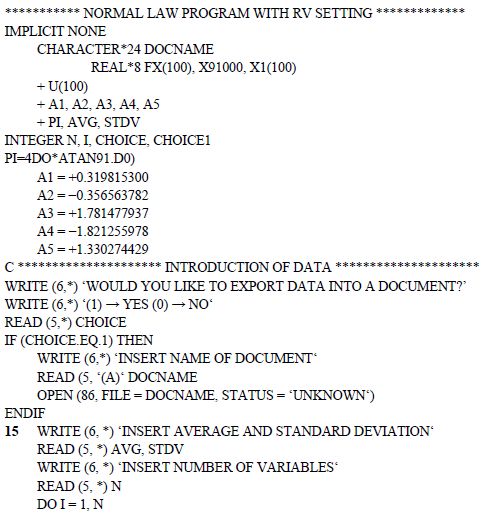
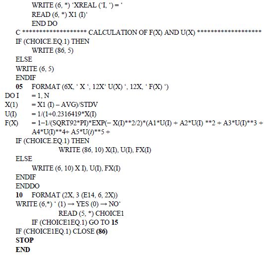
Table 7.5. Results: X, u(X) and f(X): statistical distribution laws
| X | u(X) | f(X) |
| 0.116327 E + 02 | 0.270665 E + 00 | 0.100000 E + 01 |
| −0.121076 E + 01 | 0.138978 E + 01 | 0.110584 E + 01 |
| −0.146302 E + 01 | 0.151262 E + 01 | 0.652430 E − 01 |
| −0.576923 E + 00 | 0.115425 E + 01 | 0.281909 E + 00 |
We have conducted ten simulations (n = 10, 20, 30, 40, 50, 60, 70, 80, 90, 100) by considering random variables a0 and m by their respective distributions.
Figure 7.1. Convergence of MC simulation
We can clearly see the convergence of MC simulation. We feared beforehand that there would be convergence difficulties, because we knew from the literature that one of the problems with SM was the convergence of simulated variable probability results on randomly drawn N (100 in our case).
We will now present another mathematical technique used to generate random numbers and succinctly show how we are able to approach them with our four statistical distribution laws: uniform, exponential, Gauss, and Weibull. To do this, this time we require a model programmed with the help of the MathCAD software.
This mathematical approach is used to create a vector of random numbers from three laws on a given interval: a uniform law, a normal law, and an exponential law. This mathematical technique includes two programs which allow us to control the initial value used to generate random numbers.
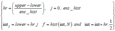
First, it is advisable to enter the number of random centered variables and to limit (set) them by their highest and lowest extremities, as follows:
| Enter highest and lowest extremities: | l0 = 2hi = 2 |
| Enter the number of groups for the histogram: | ens_hist = 20 |
| Vector of random centered variables: | N = runif(n, lo, hi) |
| Frequency distribution: | Lower = floor(min(N)) |
| upper = ceil(max(N)) | |
| n = 1x10³ |
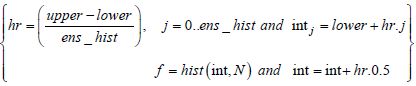
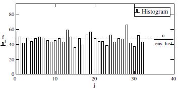
Figure 7.2. Frequency distribution of uniform law using MC simulation
| Enter the number of random centered variables: | n = 1 × 10³ |
| Enter the average and standard deviation: | μ = 0 and σ = 2 |
| Vector of random centered variables: | N = norm(n, μ, σ) |
| Frequency distribution: | Lower = floor(min(N)) |
| upper = ceil(max(N))/2 |
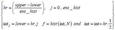
Normal adjustment function: F(x) = n.hr.dnorm(n, μ, σ)
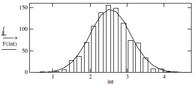
Figure 7.3. Frequency distribution of Gaussian law using MC simulation
| Enter the number of random centered variables: | n = 1 × 10³ |
| Enter the rate a: | α = 0.5 |
| Enter the number of groups for the histogram: | ens_hist = 20 |
| Vector of random centered variables: | N = rexp (n, α) |
| Frequency distribution: | Lower = floor (min (N)) |
| upper = ceil (max (N))/2 |

The following program allows us to generate the same set of random numbers following a normal law at each iteration, by resetting the initial value. Let the number of iterations n = 103 with an average µ = 0 and standard deviation σ = 2.
Figure 7.4. Frequency distribution of exponential law using MC simulation
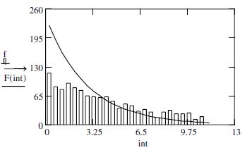
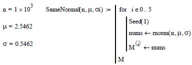
Table 7.6. Generation of random numbers following a Gaussian at each iteration (n) by resetting and controlling the initial value
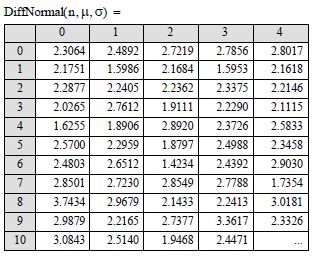
Note that the exact same set of random numbers is generated each time; each column includes the same numbers in the same order. In the same vein, this program allows us to control and to repeat the generation process with a new set of random numbers from a given initial value.

Table 7.7. Generation of random numbers following a Gaussian at each iteration (n) by resetting and controlling the initial value

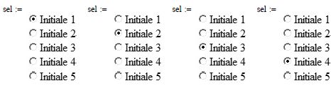
We can also represent the columns graphically to clearly observe the effects. With the help of the software MathCAD, the selection technique is as follows:

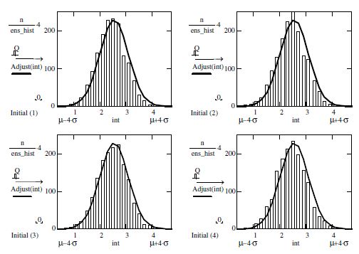
Using MathCAD software, it is possible to graphically represent these columns to observe the effects of the Gaussian curves plotted in the following for four cases of simulation:
The graphic results are presented as follows.
On this basis, we can now plot the histograms and inherent laws:
Figure 7.5. Adjustment of normal law frequencies using MC simulation
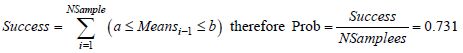
The following uses random number generators to explain how important sampling methods can estimate probabilities of quantities with unknown distributions. The estimation of an average in a logistical distribution sample is used for educational purposes.
PROBLEM.– We will demonstrate in an empirical manner that the average in the sample (based on a sample size, SSize = 100) of a logistical distribution with the parameters L and S, is located in the interval [a, b].
We will shortly present the results of the MC simulation through drawing random variables a0 and m at chance. We will calculate the failure probabilities of the structure, through welding processes, on the results from 100 drawn values. We can establish a good stability of convergence toward the 40th drawn values (see Figure 7.2).
The next stage will provide a calculated interpretation of averages and standard deviations, which we can calculate the reliability index by using a limit state function, as clarified: M = (R – S) < 0.
Third stage: The results from the MC simulation calculations, which have already been used to plot distribution functions, can be grouped by average and standard deviation.
Table 7.8. Average and standard deviations from MC simulation of variables on the number of theoretical cycles to imitate parameters a0 and m
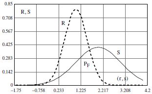
After having carried out a “setting” of functions from random variables (a0, m, and N), we can apply the method of load-stress to calculate the failure probability PF and the safety index. Our results must be similar to the following theoretical graph:
We will now attempt to answer the following question: With what probability of PF would there be certain failure, if we know its capacity R to resist load S, and what would its probable safety index βc be?
Figure 7.6. Simplification of failure probability PF according to a Gaussian distribution
To objectively answer this question we follow the following stages:
a) First stage
According to Figure 7.6, we can clearly see that it is necessary to first calculate and statistically simulate the number of cycles, by welding processes. This is what we have done until now through the simulation of random variables. Then, we can consider that the simulated Ncycles correspond to R and the “added” simulated Ncycles correspond to S.
b) Second stage
This stage involves choosing, based on an industrial demand (functional specifications), a load S which allows us to verify whether the structure will resist or break, by adding a supplementary load to the one designed at hypothesis stage. In our precise case, there is good reason to calculate a limit state function M < 0, a failure probability PF, and a safety index βc. In accordance with what has been said in this chapter so far, it would seem wise to consider a hypothesis with S > 1.5R, according to which we could calculate the failure probability PF and its safety index βc.
To do this, we must calculate and plot the probability density functions of the Ncycles, i.e. R, and on the same graph add the results from the probability density functions of load S. Graphically, the intersection of the two curves allows us to locate the failure probability as shown in Figure 7.6. Recall that analytically, the failure probability is evaluated across the limit state function M, as shown in the relationships [7.1] and [7.4]. After having defined the foundations of the random variable calculations (a0, m, and N), we will present the results of these parameters from MC simulation as follows:
Table 7.9. Calculation results for the theory of resistance and stress (R – S) < 0
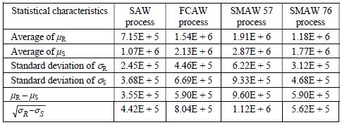
The graphical results which follow indeed correspond to the theoretical plot in Figure 7.6.
Figure 7.7. Graphical results of failure probability PF calculations, simulated according to a Gaussian distribution using MC simulation and an arbitrary choice by the engineer
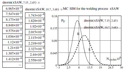
Figure 7.8. Graphical results of failure probability PF calculations, simulated according to a Gaussian distribution using MC simulation and an arbitrary choice by the engineer
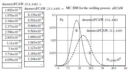
Figure 7.9. Graphical results of failure probability PF calculations, simulated according to a Gaussian distribution using MC simulation and an arbitrary choice by the engineer
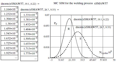
Figure 7.10. Graphical results of failure probability PF calculations, simulated according to a Gaussian distribution using MC simulation and an arbitrary choice by the engineer
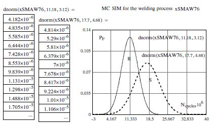
c) Third stage: graphical interpretation of probability densities arising from MC simulation (resistance/stress (R – S) < 0)
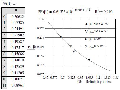
Figure 7.11. Graphical results of the safety index (β) by joining processes
We can establish on inspection of the two probability density functions that the structure will not be able to withstand the load that is imposed on it.
This process is more economic compared to traditional safety coefficient calculations, which take material physics into consideration in a direct method. This method does not have the pretence of being perfect, but it does have the merit of considering three random variables from the crack growth law [a0, (C and/or m) and N]. In terms of these results, we have calculated, by exponential regression, an average relationship which allows us to read the failure probability according to the safety index (βc) with a good correlation (R2 = 0.91).
We have presented the MC simulation method, which has allowed us to obtain very weak probabilities, in the region of 10–6 This method is relatively well adapted to singular structures because first it allows us to determine the safety index βc, which is used to design structures and constructions. Also, with very few additional calculations and without a restrictive hypothesis, it completes the independence between resistance R and load S. By knowing the Hasofer–Lind or the Cornell index, this method allows us to attain a so-called level III precision, with a few supplementary calculations. On the other hand, this method remains dependent on the random drawing of random variables a0 and m. This is what we have done throughout the examples shown in this chapter.
We are equally convinced that for 27,000 draws from the KS model, we have a convergence of failure probability. However, we note the complexity of the MC simulation method. Structural reliability analysis requires the control of structural and material behavior. It needs ample advanced knowledge in probabilistic simulation to reach a correct imitation of the random variables which intervene in the problem, in this case a0, m, and N. It also requires highly evolved mathematical techniques to carry out multidimensional integrations from probability densities and zones of failure (M < 0).
The method of using pseudo-random simulations has clearly spread to the study of safety in numerous fields. The most commonly used technique in civil engineering is the MC simulations technique. This very general technique is simple to put into place: in this chapter we have provided its principal features. The issue that these techniques raise (which is dealt with in the following chapter) is their convergence rate toward a stable and faintly variant result, when this result is a failure probability, and therefore very weak. Technical literature (informatics programs) on numerous pseudo-random algorithms provides uniformly distributed values. A very widespread class of generators uses a linear congruence. For our part, we have used programs from the software MathCAD rather than the Fibonacci suite.
[AME 84] AMERICAN WELDING SOCIETY, “Structural welding code”, AWS DI, pp. 1–84, 1984.
[API 87] API, AMERICAN PETROLEUM INSTITUTE RECOMMENDED PRACTICE FOR PLANNING, DESIGN AND CONSTRUCTION OF FIXED OFFSHORE STRUCTURES, API RP 2A, 1987.
[BAS 60] BASLER E., “Analysis of structural safety”, Paper presented to the ASCE Annual Convention, Boston, MA, June 1960.
[CAD 84] CADIOU J., “Conception des produits industriels; méthodes et moyens”, Étude de la Fiabilité d’un projet, Techniques de l’ingénieur, page T-4 301–4, Paris, France, 1984.
[CIR 77] CIRIA CONSTRUCTION INDUSTRY RESEARCH AND INFORMATION ASSOCIATION, Rationalisation of safety and serviceability factors in structural codes, CIRIA Report numb. 63, UK, London, 1977.
[CIR 81] CIRIA CONSTRUCTION INDUSTRY RESEARCH AND INFORMATION ASSOCIATION, Design for movement in buildings, Series/doc. no. Technical Note TN 107, UK, London, 1981.
[COR 67] CORNELL C.A., “Bounds on reliability of structural systems”, ASCE/STI, vol. 93, pp. 171–200, 1967.
[COR 69] CORNELL C.A., “A Probability-based on structural code”, Journal of the American Concrete Institute, vol. 66, no. 12, pp. 974–985, 1969.
[CSA 81] CSA (Canadian Standardization Association), Standards for the Design of Cold-Formed Steel Members in Building, CSA S-136, 1974–1981.
[CSA 11] CSA (Canadian Standardization Association), Norme canadienne sur la procédure de contrôle opérationnel en soudage, W47.2-2011, CWB (Canadian Welding Bureau), 4 April 2011.
[DIT 73] DITLEVSEN O., Structural reliability and invariance problem, Research Report No. 22, Solid Mechanics Division, University of Waterloo, Canada, 1973.
[DIT 79] DITLEVSEN O., “Narrow reliability bounds for structures systems”, Journal Structures Mechanics, vol. 7, no. 4, pp. 453–472, 1979.
[DIT 81] DITLEVSEN O. Reliability bounds for series systems with highly correlated failure modes, DCAMM Report No. 207, Technical University of Denmark, 1981.
[DIT 86a] DITLEVSEN O., OLESEN R., “Statistical analysis of virkler data on fatigue crack growth”, Engineering Fracture Mechanics, vol. 25, no. 2, pp. 177–195, 1986.
[DIT 86b] DITLEVSEN O., BJERAGER P., “Methods of structural systems reliability”, Structural Safety, 3, pp. 195–229, Technical University of Denmark, Elsevier Science, 1986.
[DnV 82] DETNORSKEVERITAS (DNV), “Rules for Design, Construction and Inspection of Offshore Structures”, Appendix C Steel Structures, Reprint with Corrections, 1982.
[ENG 82] ENGESVIK M.K., Analysis of uncertainties in fatigue capacity of welded joints, Report UR-82-17, Institute of Technology, University of Trondheim, Norway, 1982.
[FOG 82] FOGLI M., LEMAIRE M., SAINT-ANDRÉ M., “L’approche de Monte Carlo dans les problèmes de sécurité”, Annales de L’ITBTP 04–04, France, 1982.
[FRE 47] FREUDENTHAL A.M., “The safety of structures”, Transactions of ASCE, vol. 112, 1947.
[FRE 66] FREUDENTHAL A.M., GARRELTS J.M., SHINOZUKA M., “The analysis of structural safety”, Journal of Structural division, Proceedings of ASCE, STI, vol. 92, pp. 267–325, 1966.
[GRO 11] GROUS A., Applied Metrology for Manufacturing Engineering, ISTE Ltd., London, and John Wiley & Sons, Inc., New York, 2011.
[GRO 94] GROUS A., Étude probabiliste du comportement des Matériaux et structure d’un joint en croix soudé, PhD thesis, UHA, France, 1994.
[GRO 98] GROUS A., RECHO N., LASSEN T., LIEURADE H.P., “Caractéristiques mécaniques de fissuration et défaut initial dans les soudures d’angles en fonction du procédé de soudage”, Revue Mécanique Industrielle et Matériaux, Paris, vol. 51, no. 1, April 1998.
[HAS 74] HASOFER A.M., LIND N.C., “An exact and invariant first-order reliability format (FORM)”, Journal of Engineering Mechanics, ASCE, vol. 100, (EMI), pp. 111–121, 1974.
[HOH 84] HOHENBICHLER M., An asymptotic formula for the crossing rate of normal processus into intersections, Technische Universität München, Heft 75/84, 1984.
[KIU 85] DER GIUREGHIAN A., LIU P.L., “Structural reliability under incomplete probability in-formation”, Journal of Engineering Mechanics, ASCE, vol. 112, no. 1, pp. 85–104, 1986.
[LAS 92] LASSEN T., Experimental investigation and probalistic modelling of the fatigue crack growth in welded joints, Summary Report, Agder College of Engineering., Grimstad, 1992.
[LIN 73] LIND N.C., “The design of the structural design norm”, Journal of Structural Mechanics, vol. 1, no. 3. pp. 357–370, 1973.
[LIU 86] LIU P.L., DER GIUREGHIAN A., “Multivariate distribution models with prescribed marginals and covariances”, Probabilistic Engineering Mechanics, vol. 1, no. 2, pp. 105–112, 1986.
[LIU 91] LIU P.L., DER GIUREGHIAN A., “Optimization algorithms for structural reliability”, Structural Safety, vol. 9, no. 3, pp. 161–177, 1991.
[NEU 51] VON NEUMANN J., Simulation Various Techniques Used in Connection with Random Digit, U.S. National Bureau of Standards: Applied Mathematics Series, no. 12, pp. 36–38, 1951.
[PRO 87] PROVAN J.W. (Ed.), “Probabilistic fracture mechanics and reliability”, in Engineering Application of Fracture Mechanics (EAFM), Nijhoff, McGill University, MTL, Canada, 1987.
[RAV 73] RAVINDRA M.K., LIND N.C., “Safety, theory of structural code optimization”, Journal of the Structural Division, ASCE, vol. 99, pp. 541–553, 1973.
[RUB 81] RUBINSTEIN Y., Simulation and the Monte Carlo Method, John Wiley & Sons, Inc., 1981.
[SCH 79] SCHUËLLER G.I., KAFKA P., SHMITT W., “Some aspects of the iteration between systems and structural reliability”, Fifth International Conference on Structural Mechanics in Reactor Technology, Invited paper (M8/1*), Berlin, August 12–19, 1979.
[SCH 87] SCHÜELLER G.I., SHINOZUKA M., Stochastic Methods in Structural Dynamic, Nijhoff, 1987.
[SEL 93] SELLIER A., MEBARKI A., “Évaluation de la probabilité d’occurrence d’un évènement rare par utilisation du tirage d’importance conditionné”, Annales des Ponts et Chaussées, 3ème trimestre, 1993.
[SIG 77] SIGN O., “Factors affecting the fatigue strength of erlded high strength steels”, British Welding Journal, pp. 108–116, March 1977.
[WEI 39] WEIBULL W., A Statistical Theory of the Strength of Materials, Royal Swedish Institute of Engineering Research, No. 151, Stockholm, Sweden, 1939.