III Time Series, Information, and Communication
There is a large class of phenomena in which what is observed is a numerical quantity, or a sequence of numerical quantities, distributed in time. The temperature as recorded by a continuous recording thermometer, or the closing quotations of a stock in the stock market, taken day by day, or the complete set of meteorological data published from day to day by the Weather Bureau are all time series, continuous or discrete, simple or multiple. These time series are relatively slowly changing, and are well suited to a treatment employing hand computation or ordinary numerical tools such as slide rules and computing machines. Their study belongs to the more conventional parts of statistical theory.
What is not generally realized is that the rapidly changing sequences of voltages in a telephone line or a television circuit or a piece of radar apparatus belong just as truly to the field of statistics and time series, although the apparatus by means of which they are combined and modified must in general be very rapid in its action, and in fact must be able to put out results pari passu with the very rapid alterations of input. These pieces of apparatus—telephone receivers, wave filters, automatic sound-coding devices like the Vocoder of the Bell Telephone Laboratories, frequency-modulating networks and their corresponding receivers—are all in essence quick-acting arithmetical devices, corresponding to the whole apparatus of computing machines and schedules, and the staff of computers, of the statistical laboratory. The ingenuity needed in their use has been built into them in advance, just as it has into the automatic range finders and gun pointers of an anti-aircraft fire-control system, and for the same reasons. The chain of operation has to work too fast to admit of any human links.
One and all, time series and the apparatus to deal with them, whether in the computing laboratory or in the telephone circuit, have to deal with the recording, preservation, transmission, and use of information. What is this information, and how is it measured? One of the simplest, most unitary forms of information is the recording of a choice between two equally probable simple alternatives, one or the other of which is bound to happen—a choice, for example, between heads and tails in the tossing of a coin. We shall call a single choice of this sort a decision. If then we ask for the amount of information in the perfectly precise measurement of a quantity known to lie between A and B, which may with uniform a priori probability lie anywhere in this range, we shall see that if we put A = 0 and B = 1, and represent the quantity in the binary scale by the infinite binary number. a1 a2 a3 ... an ..., where a1, a2, ..., each has the value 0 or 1, then the number of choices made and the consequent amount of information is infinite. Here
![]() (3.01)
(3.01)
However, no measurement which we actually make is performed with perfect precision. If the measurement has a uniformly distributed error lying over a range of length · b1 b2 ... bn ..., where bk is the first digit not equal to 0, we shall see that all the decisions from a1 to ak−1, and possibly to ak, are significant, while all the later decisions are not. The number of decisions made is certainly not far from
![]() (3.02)
(3.02)
and we shall take this quantity as the precise formula for the amount of information and its definition.
We may conceive this in the following way: we know a priori that a variable lies between 0 and 1, and a posteriori that it lies on the interval (a, b) inside (0, 1). Then the amount of information we have from our a posteriori knowledge is
![]() (3.03)
(3.03)
However, let us now consider a case where our a priori knowledge is that the probability that a certain quantity should lie between x and x + dx is f1(x) dx, and the a posteriori probability is f2(x) dx. How much new information does our a posteriori probability give us?
This problem is essentially that of attaching a width to the regions under the curves y = f1(x) and y = f2(x). It will be noted that we are here assuming the variable to have a fundamental equipartition; that is, our results will not in general be the same if we replace x by x3 or any other function of x. Since f1(x) is a probability density, we shall have
![]() (3.04)
(3.04)
so that the average logarithm of the breadth of the region under f1(x) may be considered as some sort of average of the height of the logarithm of the reciprocal of f1(x). Thus a reasonable measure1 of the amount of information associated with the curve f1(x) is
![]() (3.05)
(3.05)
The quantity we here define as amount of information is the negative of the quantity usually defined as entropy in similar situations. The definition here given is not the one given by R. A. Fisher for statistical problems, although it is a statistical definition; and can be used to replace Fisher’s definition in the technique of statistics.
In particular, if f1(x) is a constant over (a, b) and is zero elsewhere,
![]() (3.06)
(3.06)
Using this to compare the information that a point is in the region (0, 1) with the information that it is in the region (a, b), we obtain for the measure of the difference
![]() (3.07)
(3.07)
The definition which we have given for the amount of information is applicable when the variable x is replaced by a variable ranging over two or more dimensions. In the two-dimensional case, f(x, y) is a function such that
![]() (3.08)
(3.08)
and the amount of information is
![]() (3.081)
(3.081)
Note that f1(x, y) is of the form ϕ(x)ψ(y) and
![]() (3.082)
(3.082)
then
![]() (3.083
(3.083
and
 (3.084)
and the amount of information from independent sources is additive. An interesting problem is that of determining the information gained by fixing one or more variables in a problem. For example, let us suppose that a variable u lies between x and x + dx with the probability ![]() , while a variable v lies between the same two limits with a probability
, while a variable v lies between the same two limits with a probability ![]() . How much information do we gain concerning u if we know that u + v = w? In this case, it is clear that u = w − v, where w is fixed. We assume the a priori distributions of u and v to be independent. Then the a posteriori distribution of u is proportional to
. How much information do we gain concerning u if we know that u + v = w? In this case, it is clear that u = w − v, where w is fixed. We assume the a priori distributions of u and v to be independent. Then the a posteriori distribution of u is proportional to
![]() (3.09)
(3.09)
where c1 and c2 are constants. They both disappear in the formula for the gain in information given by the fixing of w.
The excess of information concerning x when we know w to be that which we have in advance is
 (3.091)
Note that this expression (Eq. 3.091) is positive, and that it is independent of w. It is one-half the logarithm of the ratio of the sum of the mean squares of u and v to the mean square of v. If v has only a small range of variation, the amount of information concerning u which a knowledge of u + v gives is large, and it becomes infinite as b goes to 0.
We can consider this result in the following light: let us treat u as a message and v as a noise. Then the information carried by a precise message in the absence of a noise is infinite. In the presence of a noise, however, this amount of information is finite, and it approaches 0 very rapidly as the noise increases in intensity.
We have said that amount of information, being the negative logarithm of a quantity which we may consider as a probability, is essentially a negative entropy. It is interesting to show that, on the average, it has the properties we associate with an entropy.
Let ϕ(x) and ψ(x) be two probability densities; then [ϕ(x) + ψ(x)]/2 is also a probability density. Then
 (3.10)
This follows from the fact that
In other words, the overlap of the regions under ϕ(x) and ψ(x) reduces the maximum information belonging to ϕ(x) + ψ(x). On the other hand, if ϕ(x) is a probability density vanishing outside (a, b),
![]() (3.12)
(3.12)
is a minimum when ϕ(x) = 1/(b − a) over (a, b) and is zero elsewhere. This follows from the fact that the logarithm curve is convex upward.
It will be seen that the processes which lose information are, as we should expect, closely analogous to the processes which gain entropy. They consist in the fusion of regions of probability which were originally distinct. For example, if we replace the distribution of a certain variable by the distribution of a function of that variable which takes the same value for different arguments, or if in a function of several variables we allow some of them to range unimpeded over their natural range of variability, we lose information. No operation on a message can gain information on the average. Here we have a precise application of the second law of thermodynamics in communication engineering. Conversely, the greater specification of an ambiguous situation, on the average, will, as we have seen, generally gain information and never lose it.
An interesting case is when we have a probability distribution with n-fold density f(x1, ..., xn) over the variables (x1, ..., xn), and where we have m dependent variables y1, ..., ym. How much information do we get by fixing these m variables? First let them be fixed between the limits y1*, y1* + dy1*; ...; ym*, ym + dym*. Let us take as a new set of variables x1, x2, ..., xn−m, y1, y2, ..., ym. Then over the new set of variables, our distribution function will be proportional to f(x1, ..., xn) over the region R given by ![]() and 0 outside. Thus the amount of information obtained by the specification of the y’s will be
and 0 outside. Thus the amount of information obtained by the specification of the y’s will be
 (3.13)
Closely related to this problem is the generalization of that which we discussed in Eq. 3.13; in the case just discussed, how much information do we have concerning the variables x1, ..., xn−m alone? Here the a priori probability density of these variables is
![]() (3.14)
(3.14)
and the un-normalized probability density after fixing the y*’s is
![]() (3.141)
(3.141)
where the ∑ is taken over all sets of points (xn−m+1, ..., xn) corresponding to a given set of y*’s. On this basis, we may easily write down the solution to our problem, though it will be a bit lengthy. If we take the set x1, ..., xn−m) to be a generalized message, the set (xn−m+1, ..., xm) to be a generalized noise, and the y*’s to be a generalized corrupted message, we see that we have given the solution of a generalization of the problem of Expression 3.141.
We have thus at least a formal solution of a generalization of the message-noise problem which we have already stated. A set of observations depends in an arbitrary way on a set of messages and noises with a known combined distribution. We wish to ascertain how much information these observations give concerning the messages alone. This is a central problem of communication engineering. It enables us to evaluate different systems, such as amplitude modulation or frequency modulation or phase modulation, as far as their efficiency in transmitting information is concerned. This is a technical problem and not suitable to a detailed discussion here; however, certain remarks are in order. In the first place, it can be shown that with the definition of information given here, with a random “static” on the ether equidistributed in frequency as far as power is concerned, and with a message restricted to a definite frequency range and a definite power output for this range, no means of transmission of information is more efficient than amplitude modulation, although other means may be as efficient. On the other hand, the information transmitted by this means is not necessarily in the form most suitable for reception by the ear or by any other given receptor. Here the specific characteristics of the ear and of other receptors must be considered by employing a theory very similar to the one just developed. In general, the efficient use of amplitude modulation or any other form of modulation must be supplemented by the use of decoding devices adequate to transforming the received information into a form suitable for reception by human receptors or use by mechanical receptors. Similarly, the original message must be coded for the greatest compression in transmission. This problem has been attacked, at least in part, in the design of the “Vocoder” system by the Bell Telephone Laboratories, and the relevant general theory has been presented in a very satisfactory form by Dr. C. Shannon of those laboratories.
So much for the definition and technique of measuring information. We shall now discuss the way in which information may be presented in a form homogeneous in time. Let it be noted that most of the telephone and other communication devices are actually not attached to a particular origin in time. There is indeed one operation which seems to contradict this, but which really does not. This is the operation of modulation. This, in its simplest form, converts a message f(t) into one of the form f(t) sin (at + b). If, however, we regard the factor sin (at + b) as an extra message which is put into the apparatus, it will be seen that the situation will come under our general statement. The extra message, which we call the carrier, adds nothing to the rate at which the system is carrying information. All the information it contains is conveyed in an arbitrarily short interval of time, and thereafter nothing new is said.
A message homogeneous in time, or, as the statisticians call it, a time series which is in statistical equilibrium, is thus a single function or a set of functions of the time, which forms one of an ensemble of such sets with a well-defined probability distribution, not altered by the change of t to t + τ throughout. That is, the transformation group consisting of the operators Tλ which change f(t) into f(t + λ) leaves the probability of the ensemble invariant. The group satisfies the properties that
![]() (3.15)
(3.15)
It follows from this that if Φ[f(t)] is a “functional” of f(t)—that is, a number depending upon the whole history of f(t)—and if the average of f(t) over the whole ensemble is finite, we are in a position to use the Birkhoff ergodic theorem quoted in the previous chapter, and to come to the conclusion that, except for a set of values of f(t) of zero probability, the time-average of Φ[f(t)], or in symbols,
![]() (3.16)
(3.16)
exists.
There is even more here than this. We have stated in the previous chapter another theorem of ergodic character, due to von Neumann, which states that, except for a set of elements of zero probability, any element belonging to a system which goes into itself under a group of measure-preserving transformations such as Eq. 3.15 belongs to a sub-set (which may be the whole set) which goes into itself under the same transformation, which has a measure defined over itself and also invariant under the transformation, and which has the further property that any portion of this sub-set with measure preserved under the group of transformations either has the maximum measure of the sub-set, or measure 0. If we discard all elements except those of such a sub-set, and use its appropriate measure, we shall find that the time average (Eq. 3.16) is in almost all cases the average of Φ[f(t)] over all the space of functions f(t); the so-called phase average. Thus in the case of such an ensemble of functions f(t), except in a set of cases of zero probability, we can deduce the average of any statistical parameter of the ensemble—indeed we can simultaneously deduce any countable set of such parameters of the ensemble—from the record of any one of the component time series, by using a time average instead of a phase average. Moreover, we need to know only the past of almost any one time series of the class. In other words, given the entire history up to the present of a time series known to belong to an ensemble in statistical equilibrium, we can compute with probable error zero the entire set of statistical parameters of an ensemble in statistical equilibrium to which that time series belongs. Up to here, we have formulated this for single time series; it is equally true, however, for multiple time series in which we have several quantities varying simultaneously, rather than a single varying quantity.
We are now in a position to discuss various problems belonging to time series. We shall confine our attention to those cases where the entire past of a time series can be given in terms of a countable set of quantities. For example, for quite a wide class of functions f(t) (−∞ < t < ∞), we have fully determined f when we know the set of quantities
![]() (3.17)
(3.17)
Now let A be some function of the values of t in the future, that is, for arguments greater than 0. Then we can determine the simultaneous distribution of (a0, a1, ..., an, A) from the past of almost any single time series if the set of f’s is taken in its narrowest possible sense. In particular, if a0, ..., an are all given, we may determine the distribution of A. Here we appeal to the known theorem of Nikodym on conditional probabilities. The same theorem will assure us that this distribution, under very general circumstances, will tend to a limit as n → ∞ and this limit will give us all the knowledge there is concerning the distribution of any future quantity. We may similarly determine the simultaneous distribution of values of any set of future quantities, or any set of quantities depending both on the past and the future, when the past is known. If then we have given any adequate interpretation to the “best value” of any of these statistical parameters or sets of statistical parameters—in the sense, perhaps, of a mean or a median or a mode—we can compute it from the known distribution, and obtain a prediction to meet any desired criterion of goodness of prediction. We can compute the merit of the prediction, using any desired statistical basis of this merit—mean square error or maximum error or mean absolute error, and so on. We can compute the amount of information concerning any statistical parameter or set of statistical parameters, which fixing of the past will give us. We can even compute the whole amount of information which a knowledge of the past will give us of the whole future beyond a certain point; although when this point is the present, we shall in general know the latter from the past, and our knowledge of the present will contain an infinite amount of information.
Another interesting situation is that of a multiple time series, in which we know precisely only the pasts of some of the components. The distribution of any quantity involving more than these pasts can be studied by means very similar to those already suggested. In particular, we may wish to know the distribution of a value of another component, or a set of values of other components, at some point of time, past, present, or future. The general problem of the wave filter belongs to this class. We have a message, together with a noise, combined in some way into a corrupted message, of which we know the past. We also know the statistical joint distribution of the message and the noise as time series. We ask for the distribution of the values of the message at some given time, past, present, and future. We then ask for an operator on the past of the corrupted message which will best give this true message, in some given statistical sense. We may ask for a statistical estimate of some measure of the error of our knowledge of the message. Finally, we may ask for the amount of information which we possess concerning the message.
There is one ensemble of time series which is particularly simple and central. This is the ensemble associated with the Brownian motion. The Brownian motion is the motion of a particle in a gas, impelled by the random impacts of the other particles in a state of thermal agitation. The theory has been developed by many writers, among them Einstein, Smoluchowski, Perrin, and the author.2 Unless we go down in the time scale to intervals so small that the individual impacts of the particles on one another are discernible, the motion shows a curious kind of undifferentiability. The mean square motion in a given direction over a given time is proportional to the length of that time, and the motions over successive times are completely uncorrelated. This conforms closely to the physical observations. If we normalize the scale of the Brownian motion to fit the time scale, and consider only one coordinate x of the motion, and if we let x(t) equal 0 for t = 0, then the probability that if ![]() the particles lie between x1 and x1 + dx1 at time t1, ..., between xn and xn + dxn at time tn, is
the particles lie between x1 and x1 + dx1 at time t1, ..., between xn and xn + dxn at time tn, is
 (3.18)
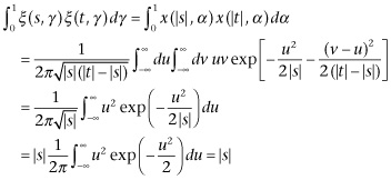
On the basis of the probability system corresponding to this, which is unambiguous, we can make the set of paths corresponding to the different possible Brownian motions depend on a parameter α lying between 0 and 1, in such a way that each path is a function x(t, α), where x depends on the time t and the parameter of distribution α, and where the probability that a path lies in a certain set S is the same as the measure of the set of values of α corresponding to paths in S. On this basis, almost all paths will be continuous and non-differentiable.
A very interesting question is that of determining the average with respect to α of x(t1, α) ... x(tn, α). This will be
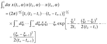 (3.19)
under the assumption that ![]() , Let us put
, Let us put
![]() (3.20)
(3.20)
where λk,1 + λk,2 + ··· + λk,n = n. The value of the expression in Eq. 3.19 will become
 (3.21)
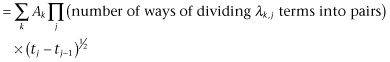

![]()
Here the first ∑ sums over j; the second, over all the ways of dividing n terms in blocks, respectively, of λk,1, ..., λk,n numbers into pairs; and the ∏ is taken over those pairs of values k and q, where λk,1 of the elements to be selected from tk and tq are t1, λk,2 are t2, and so on. It immediately results that
![]() (3.22)
(3.22)
where the ∑ is taken over all partitions of t1, ..., tn into distinct pairs, and the ∏ over all the pairs in each partition. In other words, when we know the averages of the products of x(tj, α) by pairs, we know the averages of all polynomials in these quantities, and thus their entire statistical distribution.
Up to the present, we have considered Brownian motions x(t, α) where t is positive. If we put
![]() (3.23)
(3.23)
where α and β have independent uniform distributions over (0, 1), we shall obtain a distribution of ξ(t, α, β) where t runs over the whole real infinite line. There is a well-known mathematical device to map a square on a line segment in such a way that area goes into length. All we need to do is to write our coordinates in the square in the decimal form:
![]() (3.24)
(3.24)
and to put
![]()
and we obtain a mapping of this sort which is one-one for almost all points both in the line segment and the square. Using this substitution, we define
![]() (3.25)
(3.25)
We now wish to define
![]() (3.26)
(3.26)
The obvious thing would be to define this as a Stieltjes3 integral, but ξ is a very irregular function of t and does not make such a definition possible. If, however, K runs sufficiently rapidly to 0 at ± ∞ and is a sufficiently smooth function, it is reasonable to put
![]() (3.27)
(3.27)
Under these circumstances, we have formally
 (3.28)
Now, if s and t are of opposite signs,
while if they are of the same sign, and |s| < |t|,
 (3.30)
Thus:
 (3.31)
In particular,
 (3.32)
Moreover,
 (3.33)
where the sum is over all partitions of τl, ..., τn into pairs, and the product is over the pairs in each partition.
The expression
![]() (3.34)
(3.34)
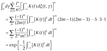
represents a very important ensemble of time series in the variable t, depending on a parameter of distribution γ. We have just shown what amounts to the statement that all the moments and hence all the statistical parameters of this distribution depend on the function
 (3.35)
which is the statisticians’ autocorrelation function with lag τ. Thus the statistics of distribution of f(t, γ) are the same as the statistics of f(t + t1, γ); and it can be shown in fact that, if
![]() (3.36)
(3.36)
then the transformation of γ into Γ preserves measure. In other words, our time series f(t, γ) is in statistical equilibrium.
Moreover, if we consider the average of
![]() (3.37)
(3.37)
it will consist of precisely the terms in
![]() (3.38)
(3.38)
together with a finite number of terms involving as factors powers of
![]() (3.39)
(3.39)
and if this approaches 0 when σ → ∞, Expression 3.38 will be the limit of Expression ‘3.37 under these circumstances. In other words, f(t, γ) and f(t + σ, γ) are asymptotically independent in their distributions as σ → ∞. By a more generally phrased but entirely similar argument, it may be shown that the simultaneous distribution of f(t1, γ), ..., f(tn, γ) and of f(σ + s1, γ), ..., f(σ + sm, γ) tends to the joint distribution of the first and the second set as σ → ∞. In other words, any bounded measurable functional or quantity depending on the entire distribution of the values of the function of t, f(t, γ), which we may write in the form ![]() , must have the property that
, must have the property that
![]() (3.40)
(3.40)
If now ![]() is invariant under a translation of t, and only takes on the values 0 or 1, we shall have
is invariant under a translation of t, and only takes on the values 0 or 1, we shall have
![]() (3.41)
(3.41)
so that the transformation group of f(t, γ) into f(t + σ, γ) is metrically transitive. It follows that if ![]() is any integrable functional of f as a function of t, then by the ergodic theorem
is any integrable functional of f as a function of t, then by the ergodic theorem
 (3.42)
for all values of γ except for a set of zero measure. That is, we can almost always read off any statistical parameter of such a time series, and indeed any denumerable set of statistical parameters, from the past history of a single example. Actually, for such a time series,
when we know
![]() (3.43)
(3.43)
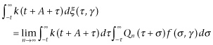
we know Φ(t) in almost every case, and we have a complete statistical knowledge of the time series.
There are certain quantities dependent on a time series of this sort which have quite interesting properties. In particular, it is interesting to know the average of
![]() (3.44)
(3.44)
Formally, this may be written
 (3.45)
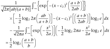
It is a very interesting problem to try to build up a time series as general as possible from the simple Brownian motion series. In such constructions, the example of the Fourier developments suggests that such expansions as Expression 3.44 are convenient building blocks for this purpose. In particular, let us investigate time series of the special form
Let us suppose that we know ξ(τ, γ) as well as Expression 3.46. Then, as in Eq. 3.45, if t1 > t2,
 (3.47)
If we now multiply by exp[s2(t2 − t1)/2], let s(t2 − t1) = iσ, and let t2 → t1, we obtain
![]() (3.48)
(3.48)
Let us take K(t1, λ) and a new independent variable µ and solve for λ, obtaining
![]() (3.49)
(3.49)
Then Expression 3.48 becomes
![]() (3.50)
(3.50)
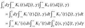
From this, by a Fourier transformation, we can determine
![]() (3.51)
(3.51)
as a function of µ, when µ, lies between K(t1, a) and K(t1, b). If we integrate this function with respect to µ, we determine
![]() (3.52)
(3.52)
as a function of K(t1, λ) and t1. That is, there is a known function F(u, v), such that
![]() (3.53)
(3.53)
Since the left-hand side of this equation does not depend on t1, we may write it G(λ), and put
![]() (3.54)
(3.54)
Here, F is a known function, and we can invert it with respect to the first argument, and put
![]() (3.55)
(3.55)
where it is also a known function. Then
![]() (3.56)
(3.56)
Then the function
![]() (3.57)
(3.57)
will be a known function, and
![]() (3.58)
(3.58)
That is,
![]() (3.59)
(3.59)
or
![]() (3.60)
(3.60)
This constant will be given by
![]() (3.61)
(3.61)
or
![]() (3.62)
(3.62)
It is easy to see that if a is finite, it does not matter what value we give it; for our operator is not changed if we add a constant to all values of λ. We can hence make it 0. We have thus determined λ as a function of G, and thus G as a function of λ. Thus, by Eq. 3.55, we have determined K(t, λ). To finish the determination of Expression 3.46, we need only know b. This can be determined, however, by a comparison of
![]() (3.63)
(3.63)
with
![]() (3.64)
(3.64)
Thus, under certain circumstances which remain to be definitely formulated, if a time series may be written in the form of Expression 3.46 and we know ξ(t, γ) as well, we can determine the function K(t, λ) in Expression 3.46 and the numbers a and b, except for an undetermined constant added to a, λ, and b. There is no extra difficulty if b = +∞, and it is not hard to extend the reasoning to the case where a = −∞. Of course, a good deal of work remains to be done to discuss the problem of the inversion of the functions inverted when the results are not single-valued, and the general conditions of validity of the expansions concerned. Still, we have at least taken a first step toward the solution of the problem of reducing a large class of time series to a canonical form, and this is most important for the concrete formal application of the theories of prediction and of the measurement of information, as we have sketched them earlier in this chapter.
There is still one obvious limitation which we should remove from this approach to the theory of time series: the necessity which we are under of knowing ξ(t, γ) as well as the time series which we are expanding in the form of Expression 3.46. The question is: under what circumstances can we represent a time series of known statistical parameters as determined by a Brownian motion; or at least as the limit in some sense or other of time series determined by Brownian motions? We shall confine ourselves to time series with the property of metrical transitivity, and with the even stronger property that if we take intervals of fixed length but remote in time, the distributions of any functionals of the segments of the time series in these intervals approach independence as the intervals recede from eachother.4 The theory to be developed here has already been sketched by the author.
If K(t) is a sufficiently continuous function, it is possible to show that the zeros of
![]() (3.65)
(3.65)
almost always have a definite density, by a theorem of M. Kac, and that this density can be made as great as we wish by a proper choice of K. Let KD be so selected that this density is D. Then the sequence of zeros of ![]() from −∞ to ∞ will be called Zn(D, γ), −∞ < n < ∞. Of course, in the numeration of these zeros, n is determined except for an additive constant integer.
from −∞ to ∞ will be called Zn(D, γ), −∞ < n < ∞. Of course, in the numeration of these zeros, n is determined except for an additive constant integer.
Now, let T(t, μ) be any time series in the continuous variable t, while μ is a parameter of distribution of the time series, varying uniformly over (0, 1). Then let
![]() (3.66)
(3.66)
where the Zn taken is the one just preceding t. It will be seen that for any finite set of values t1, t2, ..., tv of x the simultaneous distribution of TD(tκ, μ, γ) (κ = 1, 2, ..., v) will approach the simultaneous distribution of T(tκ, μ) for the same tκ’s as D → ∞, for almost every value of μ. However, TD(t, μ, γ) is completely determined by t, μ, D, and ξ(τ, γ). It is therefore not inappropriate to try to express TD(t, μ, γ), for a given D and a given μ, either directly in the form of Expression 3.46 or in some way or another as a time series which has a distribution which is a limit (in the loose sense just given) of distributions of this form.
It must be admitted that this is a program to be carried through in the future, rather than one which we can consider as already accomplished. Nevertheless, it is the program which, in the opinion of the author, offers the best hope for a rational, consistent treatment of the many problems associated with non-linear prediction, non-linear filtering, the evaluation of the transmission of information in non-linear situations, and the theory of the dense gas and turbulence. Among these problems are perhaps the most pressing facing communication engineering.
Let us now come to the prediction problem for time series of the form of Eq. 3.34. We see that the only independent statistical parameter of the time series is Φ(t), as given by Eq. 3.35; which means that the only significant quantity connected with K(t) is
![]() (3.67)
(3.67)
Let us put
![]() (3.68)
(3.68)
employing a Fourier transformation. To know K(s) is to know k(ω), and vice versa. Then
![]() (3.69)
(3.69)
Thus a knowledge of Φ(τ) is tantamount to a knowledge of k(ω)k(−ω). Since, however, K(s) is real,
![]() (3.70)
(3.70)
whence k(ω) = k(−ω). Thus |k(ω)|2 is a known function, which means that the real part of log |k(ω)| is a known function.
If we write
![]() (3.71)
(3.71)
then the determination of K(s) is equivalent to the determination of the imaginary part of log k(ω). This problem is not determinate unless we put some further restriction on k(ω). The type of restriction which we shall put is that log k(s) shall be analytic and of a sufficiently small rate of growth for ω in the upper half-plane. In order to make this restriction, k(ω) and [k(ω)−1 will be assumed to be of algebraic growth on the real axis. Then [F(ω)]2 will be even and at most logarithmically infinite, and the Cauchy principal value of
![]() (3.72)
(3.72)
will exist. The transformation indicated by Eq. 3.72, known as the Hilbert transformation, changes cos λω into sin λω and sin λω into −cos λω. Thus F(ω) + iG(ω) is a function of the form
![]() (3.73)
(3.73)
and satisfies the required conditions for log |k(ω)| in the lower half-plane. If we now put
![]() (3.74)
(3.74)
it can be shown that k(ω) is a function which, under very general conditions, is such that K(s), as defined in Eq. 3.68, vanishes for all negative arguments. Thus
![]() (3.75)
(3.75)
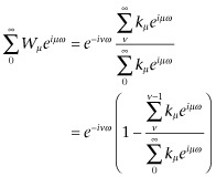
On the other hand, it can be shown that we may write 1/k(ω) in the form
![]() (3.76)
(3.76)
where the Nn’s are properly determined; and that this can be done in such a way that
![]() (3.77)
(3.77)
Here the Qn’s must have the formal property that
![]() (3.78)
(3.78)
In general, we shall have
![]() (3.79)
(3.79)
or if we write (as in Eq. 3.68)
 (3.80)
then
![]() (3.81)
(3.81)
Thus
![]() (3.82)
(3.82)
We shall find this result useful in getting the operator of prediction into a form concerning frequency rather than time.
Thus the past and present of ξ(t, γ), or properly of the “differential” dξ(t, ξ), determine the past and present of f(t, γ), and vice versa.
Now, if A > 0,
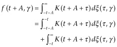 (3.83)
Here the first term of the last expression depends on a range of dξ(τ, λ) of which a knowledge of f(σ, γ) for ![]() tells us nothing, and is entirely independent of the second term. Its mean square value is
tells us nothing, and is entirely independent of the second term. Its mean square value is
![]() (3.84)
(3.84)
and this tells us all there is to know about it statistically. It may be shown to have a Gaussian distribution with this mean square value. It is the error of the best possible prediction of f(t + A, γ).
The best possible prediction itself is the last term of Eq. 3.83,
 (3.85)
If we now put
![]() (3.86)
(3.86)
and if we apply the operator of Eq. 3.85 to etωt, obtaining
![]() (3.87)
(3.87)
we shall find out (somewhat as in Eq. 3.81) that
 (3.88)
This is then the frequency form of the best prediction operator.
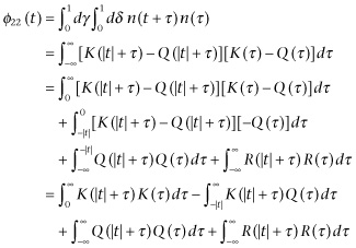
The problem of filtering in the case of time series such as Eq. 3.34 is very closely allied to the prediction problem. Let our message plus noise be of the form
![]() (3.89)
(3.89)
and let the message be of the form
![]() (3.90)
(3.90)
where γ and δ are distributed independently over (0, 1). Then the predictable part of the m(t + a) is clearly
![]() (3.901)
(3.901)
and the mean square error of prediction is
![]() (3.902)
(3.902)
Furthermore, let us suppose that we know the following quantities:
 (3.903)
 (3.904)
 (3.905)
The Fourier transforms of these three quantities are, respectively,
 (3.906)
where
 (3.907)
That is,
![]() (3.908)
(3.908)
and
![]() (3.909)
(3.909)
where for symmetry we write ![]() . We can now determine k(ω) from Eq. 3.908, as we have defined k(ω) before on the basis of Eq. 3.74. Here we put Φ(t) for
. We can now determine k(ω) from Eq. 3.908, as we have defined k(ω) before on the basis of Eq. 3.74. Here we put Φ(t) for ![]() . This will give us
. This will give us
![]() (3.910)
(3.910)
Hence
![]() (3.911)
(3.911)
and thus the best determination of m(t), with the least mean square error, is
Combining this with Eq. 3.89, and using an argument similar to the one by which we obtained Eq. 3.88, we see that the operator on m(t) + n(t) by which we obtain the “best” representation of m(t + a), if we write it on the frequency scale, is
![]() (3.913)
(3.913)
This operator constitutes a characteristic operator of what electrical engineers know as a wave filter. The quantity a is the lag of the filter. It may be either positive or negative; when it is negative, −a is known as the lead. The apparatus corresponding to Expression 3.913 may always be constructed with as much accuracy as we like. The details of its construction are more for the specialist in electrical engineering than for the reader of this book. They may be found elsewhere.5
The mean square filtering error (Expression 3.902) may be represented as the sum of the mean square filtering error for infinite lag:
 (3.914)
and a part dependent on the lag:
It will be seen that the mean square error of filtering is a monotonely decreasing function of lag.
Another question which is interesting in the case of messages and noises derived from the Brownian motion is the matter of rate of transmission of information. Let us consider for simplicity the case where the message and the noise are incoherent, that is, when
![]() (3.916)
(3.916)
In this case, let us consider
 (3.917)
where γ and δ are distributed independently. Let us suppose we know m(t) + n(t) over (−A, A); how much information do we have concerning m(t)? Note that we should heuristically expect that it would not be very different from the amount of information concerning
![]() (3.918)
(3.918)
which we have when we know all values of
![]() (3.919)
(3.919)
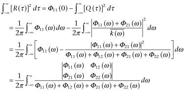
where γ and δ have independent distributions. It can, however, be shown that the nth Fourier coefficient of Expression 3.918 has a Gaussian distribution independent of all the other Fourier coefficients, and that its mean square value is proportional to
Thus, by Eq. 3.09, the total amount of information available concerning M is
 (3.921)
and the time density of communication of energy is this quantity divided by 2A. If now A → ∞, Expression 3.921 approaches
 (3.922)
This is precisely the result which the author and Shannon have already obtained for the rate of transmission of information in this case. As will be seen, it depends not only on the width of the frequency band available for transmitting the message but also on the noise level. As a matter of fact, it has a close relation to the audiograms used to measure the amount of hearing and loss of hearing in a given individual. Here the abscissa is frequency, the ordinate of lower boundary is the logarithm of the intensity of the threshold of audible intensity—what we may call the logarithm of the intensity of the internal noise of the receiving system—and the upper boundary, the logarithm of the intensity of the greatest message the system is suited to handle. The area between them, which is a quantity of the dimension of Expression 3.922, is then taken as a measure of the rate of transmission of information with which the ear is competent to cope.
The theory of messages depending linearly on the Brownian motion has many important variants. The key formulae are Eqs. 3.88 and 3.914 and Expression 3.922, together, of course, with the definitions necessary to interpret these. There are a number of variants of this theory. First: the theory gives us the best possible design of predictors and of wave filters in the case in which the messages and the noises represent the response of linear resonators to Brownian motions; but in much more general cases, they represent a possible design for predictors and filters. This will not be an absolute best possible design, but it will minimize the mean square error of prediction and filtering, in so far as this can be done with apparatus performing linear operations. However, there will generally be some non-linear apparatus which gives a performance still better than that of any linear apparatus.
Next, the time series here have been simple time series, in which a single numerical variable depends on the time. There are also multiple time series, in which a number of such variables depend simultaneously on the time; and it is these which are of greatest importance in economics, meteorology, and the like. The complete weather map of the United States, taken from day to day, constitutes such a time series. In this case, we have to develop a number of functions simultaneously in terms of the frequency, and the quadratic quantities such as Eq. 3.35 and the |k(ω)|2 of the arguments following Eq. 3.70 are replaced by arrays of pairs of quantities—that is, matrices. The problem of determining k(ω) in terms of |k(ω)|2, in such a way as to satisfy certain auxiliary conditions in the complex plane, becomes much more difficult, especially as the multiplication of matrices is not a permutable operation. However, the problems involved in this multidimensional theory have been solved, at least in part, by Krein and the author.
The multidimensional theory represents a complication of the one already given. There is another closely related theory which is a simplification of it. This is the theory of prediction, filtering, and amount of information in discrete time series. Such a series is a sequence of functions fn(α) of a parameter a, where n runs over all integer values from −∞ to ∞. The quantity a is as before the parameter of distribution, and may be taken to run uniformly over (0, 1). The time series is said to be in statistical equilibrium when the change of n to n + ν (ν an integer) is equivalent to a measure-preserving transformation into itself of the interval (0, 1) over which α runs.
The theory of discrete time series is simpler in many respects than the theory of the continuous series. It is much easier, for instance, to make them depend on a sequence of independent choices. Each term (in the mixing case) will be representable as a combination of the previous terms with a quantity independent of all previous terms, distributed uniformly over (0, 1), and the sequence of these independent factors may be taken to replace the Brownian motion which is so important in the continuous case.
If fn(α) is a time series in statistical equilibrium, and it is metrically transitive, its autocorrelation coefficient will be
![]() (3.923)
(3.923)
and we shall have
 (3.924)
for almost all α. Let us put
or
![]() (3.926)
(3.926)
Let
![]() (3.927)
(3.927)
and let
![]() (3.928)
(3.928)
Let
![]() (3.929)
(3.929)
Then under very general conditions, k(ω) will be the boundary value on the unit circle of a function without zeros or singularities inside the unit circle if ω is the angle. We shall have
![]() (3.930)
(3.930)
If now we put for the best linear prediction of fn(α) with a lead of ν
![]() (3.931)
(3.931)
we shall find that
![]() (3.932)
(3.932)
This is the analogue of Eq. 3.88. Let us note that if we put
then
 (3.934)
It will clearly be the result of the way we have formed k(ω) that in a very general set of cases we can put
![]() (3.935)
(3.935)
Then Eq. 3.934 becomes
![]() (3.936)
(3.936)
In particular, if ν = 1,
![]() (3.937)
(3.937)
or
![]() (3.938)
(3.938)
Thus for a prediction one step ahead, the best value for fn+1(α) is
![]() (3.939)
(3.939)
and by a process of step-by-step prediction, we can solve the entire problem of linear prediction for discrete time series. As in the continuous case, this will be the best prediction possible by any method if
![]() (3.940)
(3.940)
The transfer of the filtering problem from the continuous to the discrete case follows much the same lines of argument. Formula 3.913 for the frequency characteristic of the best filter takes the form
![]() (3.941)
(3.941)
where all the terms receive the same definitions as in the continuous case, except that all integrals on ω or u are from −π to π instead of from −∞ to ∞ and all sums on v are discrete sums instead of integrals on t. The filters for discrete time series are usually not so much physically constructible devices to be used with an electric circuit as mathematical procedures to enable statisticians to obtain the best results with statistically impure data.
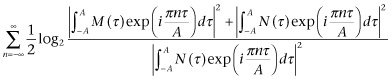
Finally, the rate of transfer of information by a discrete time series of the form
![]() (3.942)
(3.942)
in the presence of a noise
![]() (3.943)
(3.943)
when γ and δ are independent, will be the precise analogue of Expression 3.922, namely,
 (3.944)
where over (−π, π),
![]() (3.945)
(3.945)
represents the power distribution of the message in frequency, and
![]() (3.946)
(3.946)
that of the noise.
The statistical theories we have here developed involve a full knowledge of the pasts of the time series we observe. In every case, we have to be content with less, as our observation does not run indefinitely into the past. The development of our theory beyond this point, as a practical statistical theory, involves an extension of existing methods of sampling. The author and others have made a beginning in this direction. It involves all the complexities of the use either of Bayes’ law, on the one hand, or of those terminological tricks in the theory of likelihood,6 on the other, which seem to avoid the necessity for the use of Bayes’ law but which in reality transfer the responsibility for its use to the working statistician, or the person who ultimately employs his results. Meanwhile, the statistical theorist is quite honestly able to say that he has said nothing which is not perfectly rigorous and unimpeachable.
Finally, this chapter should end with a discussion of modern quantum mechanics. These represent the highest point of the invasion of modern physics by the theory of time series. In the Newtonian physics, the sequence of physical phenomena is completely determined by its past and in particular by the determination of all positions and momenta at any one moment. In the complete Gibbsian theory, it is still true that with a perfect determination of the multiple time series of the whole universe the knowledge of all positions and momenta at any one moment would determine the entire future. It is only because these are ignored, non-observed coordinates and momenta that the time series with which we actually work take on the sort of mixing property with which we have become familiar in this chapter, in the case of time series derived from the Brownian motion. The great contribution of Heisenberg to physics was the replacement of this still quasi-Newtonian world of Gibbs by one in which the time series can in no way be reduced to an assembly of determinate threads of development in time. In quantum mechanics, the whole past of an individual system does not determine the future of that system in any absolute way but merely the distribution of possible futures of the system. The quantities which the classical physics demands for a knowledge of the entire course of a system are not simultaneously observable, except in a loose and approximate way, which nevertheless is sufficiently precise for the needs of the classical physics over the range of precision where it has been shown experimentally to be applicable. The conditions of the observation of a momentum and its corresponding position are incompatible. To observe the position of a system as precisely as possible, we must observe it with light or electron waves or similar means of high resolving power, or short wavelength. However, the light has a particle action depending on its frequency only, and to illuminate a body with high-frequency light means to subject it to a change in its momentum which increases with the frequency. On the other hand, it is low-frequency light that gives the minimum change in the momenta of the particles it illuminates, and this has not a sufficient resolving power to give a sharp indication of positions. Intermediate frequencies of light give a blurred account both of positions and of momenta. In general, there is no set of observations conceivable which can give us enough information about the past of a system to give us complete information as to its future.
Nevertheless, as in the case of all ensembles of time series, the theory of the amount of information which we have here developed is applicable, and consequently the theory of entropy. Since, however, we now are dealing with time series with the mixing property, even when our data are as complete as they can be, we find that our system has no absolute potential barriers, and that in the course of time any state of the system can and will transform itself into any other state. However, the probability of this depends in the long run on the relative probability or measure of the two states. This turns out to be especially high for states which can be transformed into themselves by a large number of transformations, for states which, in the language of the quantum theorist, have a high internal resonance, or a high quantum degeneracy. The benzene ring is an example of this, since the two states are equivalent. This suggests that in a system in which various building blocks may combine themselves intimately in various ways, as when a mixture of amino acids organizes itself into protein chains, a situation where many of these chains are alike and go through a stage of close association with one another may be more stable than one in which they are different. It was suggested by Haldane, in a tentative manner, that this may be the way in which genes and viruses reproduce themselves; and although he has not asserted this suggestion of his with anything like finality, I see no cause not to retain it as a tentative hypothesis. As Haldane himself has pointed out, as no single particle in quantum theory has a perfectly sharp individuality, it is not possible in such a case to say, with more than fragmentary accuracy, which of the two examples of a gene that has reproduced itself in this manner is the master pattern and which is the copy.
This same phenomenon of resonance is known to be very frequently represented in living matter. Szent-Györgyi has suggested its importance in the construction of muscles. Substances with high resonance very generally have an abnormal capacity for storing both energy and information, and such a storage certainly occurs in muscle contraction.
Again, the same phenomena that are concerned in reproduction probably have something to do with the extraordinary specificity of the chemical substances found in a living organism, not only from species to species but even within the individuals of a species. Such considerations may be very important in immunology.