SUPERVISED LEARNING uses labelled data to make predictions about unlabelled data. One defining characteristic of supervised learning is that the goal is prediction, rather than modelling or inference. A basic nomenclature, notation and framework for supervised learning is laid down before cross-validation is introduced. After that, a simple and yet quite effective supervised learning approach, i.e., K-nearest neighbours classification, is discussed. The famous CART (classification and regression trees) framework is discussed next, followed by the bootstrap. The bootstrap is preparatory for the use of CART for ensemble learning; specifically for random forests. The chapter concludes with another ensemble learning approach, gradient boosting using XGBoost.
Consider the situation where there is an outcome variable Y that we want to predict based on several predictor variables X1, …, Xp, which we express as a vector X = (X1, …, Xp)′. Suppose that we observe n pairs (y1, x1), …, (yn, xn) and the objective is to learn the values of “new” yn+1, …,ym for corresponding values of the predictor variables, i.e., for xn+1, …, xm. Broadly speaking, one can use the observed pairs (y1, x1), …, (yn, xn) to build a model of the form
(5.1) |
where f(x) is a function, sometimes called the learner or predictor, that takes a value xi and returns a prediction for yi, and ei is the associated error. Rearranging (5.1) gives
(5.2) |
for i = 1, …,n, which is the error incurred by using f(xi) to predict yi. Some function of (5.2) can then be used to assess how well the learner performs before we apply it to predict yi for i = n + 1, …,m. Within the supervised learning paradigm, (y1, x1), …, (yn, xn) can be thought of as the labelled data because each value xi has a corresponding “label” yi. Accordingly, the xn+1, …, xm are considered unlabelled data because there are no labels, i.e., no values yn+1, …, ym, attached to the values xn+1, …, xm.
The very general modelling approach described by (5.1) and (5.2) is quite common in data science and statistics. For example, in a regression setting with yi ∈ ℝ there are a few functions of (5.2) that are commonly used to assess how well the learner performs. These include the mean squared error (MSE)
(5.3) |
for i = 1, …,n, the root mean squared error (RMSE)
(5.4) |
for i = 1, …,n, and the median absolute error (MAE)
(5.5) |
In a binary classification setting with yi ∈ {0,1} and f(xi) ∈ {0,1}, one could use the misclassification rate to assess how well the predictor f(xi) performs. In this case, i.e., with yi ∈ {0, 1} and f(xi) ∈ {0,1}, the misclassification rate can be written
(5.6) |
for i = 1, …,n. Note that (5.6) would cease to be effective in a binary classification setting with yi ∈ {−1,1} and f(xi) ∈ {−1,1}, for instance, or in the multinomial case, i.e., where there are more than two classes. Equation (5.6) can be formulated more generally for the misclassification rate:
(5.7) |
where is an indicator function, i.e.,
For some, functions such as the misclassification rate are considered too coarse for model selection. A common alternative for binary classification is the binomial deviance, or simply deviance, which can be written
(5.8) |
where is the predicted probability of yi being equal to 1 and is generated from f(xi). The quantity in (5.8) is negative two times the maximized binomial log-likelihood (McCullagh and Nelder, 1989). The deviance is a proper scoring rule (Gneiting and Raftery, 2007), which helps ensure that the predicted probabilities fit the data well and the learner is well calibrated to the data. Many other proper scoring rules exist, such as the Brier score (Brier, 1950). Binary classification models used herein are trained on the deviance and we report it along with the misclassification rate.
Hereafter, we shall use the notation Ԑlabelled to denote a generic error function for the labelled data. In general, Ԑlabelled will take the form
(5.9) |
where g((y1, f(x1)), …, (yn, f(xn))) is a function that reflects how close f(X) is to Y for the training data; such a function is sometimes called a loss function or an error function.
When doing supervised learning, the choice of error function is very important. In regression problems, the RMSE (5.4) is the standard choice; however, the RMSE is highly sensitive to outliers because it squares the errors ei. Instead of using RMSE, we train our regression models herein to minimize the MAE (5.5). The MAE is insensitive to outliers in the outcome because the median is not affected by values in the tails of the error distribution.
The learning approach described thus far has some important limitations:
1. We have said nothing about how the predictor f(x) is constructed.
2. Constructing f(x) based on (y1, x1), …, (yn, xn) and also assessing the error Ԑlabelled based on (y1, x1), …, (yn, xn) will tend to underestimate Ԑunlabelled, i.e., the error that one would see when f(x) is applied to the unlabelled data. In other words, Ԑlabelled is a biased estimator of Ԑunlabelled.
With respect to the above list item 1., it is not possible to detail exactly how the learner f(x) is constructed because this will depend on the learning method used. However, we can say a little more about how the learner f(x) is constructed in general and doing so also serves as a response to list item 2. Rather than using all of the labelled data to build the learner f(x), the labelled data are partitioned into a training set and a test set. Then, the learner f(x) is constructed based on the training set and the error is assessed based on the test set. Of course, it is reasonable to expect the test error Ԑtest to be more reflective of Ԑunlabelled than either Ԑlabelled or the training error Ԑtraining would be.
While we have gone some way towards addressing list item 1., and seemingly addressed list item 2., we have created a third problem:
3. If we overfit f(x) to the training data, then it may not perform well on the test data and/or the unlabelled data even though the training error Ԑtraining may be very small.
The existence of list item 3. as a problem is, in the first place, reflective of the fact that the goal of supervised learning is prediction. This is a key point of difference with traditional statistical procedures, where the goal is modelling or inference — while inference can be taken to include prediction, prediction is not the goal of inference. To solve the problem described in list item 3., we need to move away from thinking only about an error and consider an error together with some way to prevent or mitigate overfitting. Finally, it is worth noting that some learning approaches are more prone to overfitting than others; see Section 5.8 for further discussion.
We have seen that the training set is used to construct a learner f(x). Now, consider how this is done. One approach is to further partition the training set into two parts, and to use one part to build lots of learners and the other to choose the “best” one. When this learning paradigm is used, the part that is used to build lots of learners is called the training set, and the part used to choose the best learner is called the validation set. Accordingly, such a learning framework is called a training-validation-test framework. Similarly, the paradigm discussed in Section 5.1 can be thought of as a training-test framework.
One longstanding objection to the training-validation-test framework is that a large dataset would be required to facilitate separate training and validation sets. There are several other possible objections, one of which centres around the sensitivity of the results to the training-validation split, which will often be equal or at least close, e.g., a 40-40-20 or 50-40-10 training-validation-test split might be used. Given the increasing ease of access to large datasets, the former objection is perhaps becoming somewhat less important. However, the latter objection remains quite valid. Rather than using the training-validation-test framework, the training-test paradigm can be used with cross-validation, which allows both training and validation within the training set.
K-fold cross-validation partitions the training set into K (roughly) equal parts. This partitioning is often done so as to ensure that the yi are (roughly) representative of the training set within each partition — this is known as stratification, and it can also be used during the training-test split. In the context of cross-validation, stratification helps to ensure that each of the K partitions is in some sense representative of the training set. On each one of K iterations, cross-validation proceeds by using K − 1 of the folds to construct the learner and the remaining fold to compute the error. Then, after all iterations are completed, the K errors are combined to give the cross-validation error.
The choice of K in K-fold cross-validation can be regarded as finding a balance between variance and bias. The variance-bias tradeoff is well known in statistics and arises from the fact that, for an estimator of a parameter,
Returning to K-fold cross-validation, choosing K = n, sometimes called leave-one-out cross-validation, results is excellent (i.e., low) bias but high variance. Lower values of K lead to more bias but less variance, e.g., K =10 and K = 5 are popular choices. In many practical examples, K = n, K = 10 and K = 5 will lead to similar results.
The following code block illustrates how one could write their own cross-validation routine in Julia. Note that this serves, in part, as an illustration of how to write code in Julia — there are, in fact, cross-validation functions available within Julia (see, e.g., Section 5.7). The first function, cvind() breaks the total number of rows in the training set, i.e., N, into k nearly equal groups. The folds object returned by the function is an array of arrays. Each sub-array contains gs randomly shuffled row indices. The last sub-array will be slightly larger than gs if k does not divide evenly into N. The second function, kfolds(), divides the input data dat into k training-test dataframes based on the indices generated by cvind(). It returns a dictionary of dictionaries, with the top level key corresponding to the cross-validation fold number and the subdictionary containing the training and test dataframes created from that fold’s indices. This code expects that dat is a dataframe and would not be efficient for dataframes with large N. In this scenario, the indices should be used to subset the data and train the supervised learners in one step, without storing all the training-test splits in a data structure.
using Random
Random.seed!(35)
## Partition the training data into K (roughly) equal parts
function cvind(N, k)
gs = Int(floor(N/k))
## randomly shuffles the indices
index = shuffle(collect(1:N))
folds = collect(Iterators.partition(index, gs))
## combines and deletes array of indices outside of k
if length(folds) > k
folds[k] = vcat(folds[k], folds[k+1])
deleteat!(folds, k+1)
end
return folds
end
## Subset data into k training/test splits based on indices
## from cvind
function kfolds(dat, ind, k)
## row indices for dat
ind1 = collect(1:size(dat)[1])
## results to return
res = Dict{Int, Dict}()
for i = 1:k
## results for each loop iteration
res2 = Dict{String, DataFrame}()
## indices not in test set
tr = setdiff(ind1, ind[i])
## add results to dictionaries
push!(res2, "tr"=>dat[tr,:])
push!(res2, "tst"=>dat[ind[i],:])
push!(res, i=>res2)
end
return res
end
5.3 Κ-NEAREST NEIGHBOURS CLASSIFICATION
The k-nearest neighbours (kNN) classification technique is a very simple supervised classification approach, where an unlabelled observation is classified based on the labels of the k closest labelled points. In other words, an unlabelled observation is assigned to the class that has the most labelled observations in its neighbourhood (which is of size k). The value of k needs to be selected, which can be done using cross-validation, and the value of k that gives the best classification rate under cross-validation is generally chosen. Note that, if different k give similar or identical classification rates, the smaller value of k is usually chosen.
The next code block shows how the kNN algorithm could be implemented in Julia. The knn() function takes arrays of numbers for the existing data and labels, the new data and a scalar for k. It uses Manhattan distance to compare each row of the existing data to a row of the new data and returns the majority vote of the labels associated with the smallest k distances between the samples. The maj_vote() function is used to calculate the majority vote, and returns the class and its proportion as an array.
## majority vote
function maj_vote(yn)
## majority vote
cm = countmap(yn)
mv = -999
lab = nothing
tot = 1e-8
for (k,v) in cm
tot += v
if v > mv
mv = v
lab = k
end
end
prop = /(mv, tot)
return [lab, prop]
end
## KNN label prediction
function knn(x, y, x_new, k)
n,p = size(x)
n2,p2 = size(x_new)
ynew = zeros(n2,2)
for i in 1:n2 ## over new x_new
res = zeros(n,2)
for j in 1:n ## over x
## manhattan distance between rows - each row is a subject
res[j,:] = [j, cityblock(x[j,:], x_new[i,:])] #cityblock
end
## sort rows by distance and index - smallest distances
res2 = sortslices(res, dims = 1, by = x -> (x[2], x[1]))
## get indices for the largest k distances
ind = convert(Array{Int}, res2[1:k, 1])
## take majority vote for the associated indices
ynew[i,:] = maj_vote(y[ind])
end
## return the predicted labels
return ynew
end
## Returns the missclassification rate
function knnmcr(yp, ya)
disagree = Array{Int8}(ya .!= yp)
mcr = mean(disagree)
return mcr
end
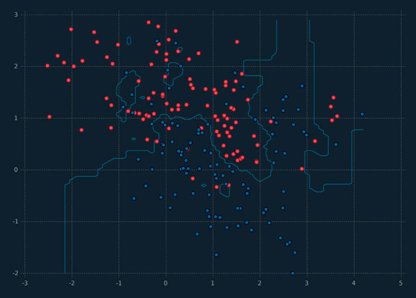
An illustration of kNN is given in Figure 5.1, where k = 3 and the neighbourhoods for each class are clearly visible. An unlabelled observation in one of the red neighbourhoods will be labelled as belonging to the red class, and similarly for the blue neighbourhood.
The next code block details how we can use the cross-validation functions already described to do 5-fold cross-validation for a kNN learner. Simulated data, df_knn which we mean centre and scale to have standard deviation one (not shown), is divided into 5 training-test splits using the cvind() and kfold() functions. We loop through the 15 values of k and, for each one, calculate the mean misclassification rate and its standard error over the 5 folds.
## Simulated data
df_3 = DataFrame(y = [0,1], size = [250,250], x1 =[2.,0.], x2 =[−1.,−2.])
df_knn =by(df_3, :y) do df
DataFrame(x_1 = rand(Normal(df[1,:x1],1), df[1,:size]),
x_2 = rand(Normal(df[1,:x2],1), df[1,:size]))
end
## set up parameters for cross-validation
N = size(df_knn) [1]
kcv = 5
## generate indices
a_ind = cvind(N, kcv)
## generate dictionary of dataframes
d_cv = kfolds(df_knn, a_ind, kcv)
## knn parameters
k = 15
knnres = zeros(k,3)
## loop through k train/test sets and calculate error metric
for i = 1:k
cv_res = zeros(kcv)
for j = 1:kcv
tr_a = convert(Matrix, d_cv[j]["tr"][[:x_1, :x_2]])
ytr_a = convert(Vector, d_cv[j]["tr"][:y])
tst_a = convert(Matrix, d_cv[j]["tst"][[:x_1, :x_2]])
ytst_a = convert(Vector, d_cv[j]["tst"][:y])
pred = knn(tr_a, ytr_a, tst_a, i)[:,1]
cv_res[j] = knnmcr(pred, ytst_a)
end
knnres[i, 1] = i
knnres[i, 2] = mean(cv_res)
knnres[i, 3] = /(std(cv_res), sqrt(kcv))
end
Figure 5.1 An illustration of kNN, for k = 3, using simulated data.
The cross-validation results are depicted in Figure 5.2. This plot shows an initial improvement in misclassification rate up to k = 5, with the smallest CV misclassification rate occurring at k = 15. For values of k from five to 15, the values oscillate up and down but remain within one standard error of k = 15. Based on these results, we would select k = 5, as it is the simplest learner that attains close to the minimum misclassification rate.
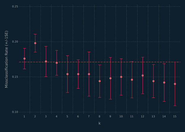
Figure 5.2 Results of 5-fold CV for 15 values of k using kNN on simulated data, where the broken line indicates one standard deviation above the minimum CV misclassification rate.
5.4 CLASSIFICATION AND REGRESSION TREES
Classification and regression trees (CART) were introduced by Breiman et al. (1984). They are relatively easy to understand and explain to a non-expert. The fact that they naturally lend themselves to straightforward visualization is a major advantage.
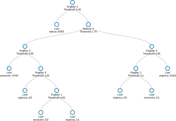
Figure 5.3 Classification tree for the iris data.
First, consider a classification tree, which starts at the top (root) and recursively partitions data based on the best splitter. A classification tree for the famous iris data is shown in Figure 5.3, where the leaves report the result (i.e., one misclassification in total). There are eight leaves: one where irises are classified as setosa, three for versicolor, and four for virginica. The representation of the tree in Figure 5.3 gives the value of the feature determining the split and the fraction of observations classified as the iris type in each leaf. Features are numbered and correspond to sepal length, sepal width, petal length, and petal width, respectively.
As we saw with the iris tree (Figure 5.3), a splitter is a variable (together with a rule), e.g.,
What it means to be the “best” splitter will be discussed, inter alia, shortly. An in-depth discussion on pruning is probably not helpful at this stage; however, there are many sources that contain such details (e.g., Breiman et al., 1984; Hastie et al., 2009). A classification tree is also known as a decision tree. Consider the notation of Hastie et al. (2009), so that a node m represents a region Rm with Nm observations. When one considers the relationship between a tree and the space of observations, this is natural. Before proceeding, consider a tree built using two variables from the iris data — two variables so that we can visualize the partitioning of the space of observations (Figure 5.4).
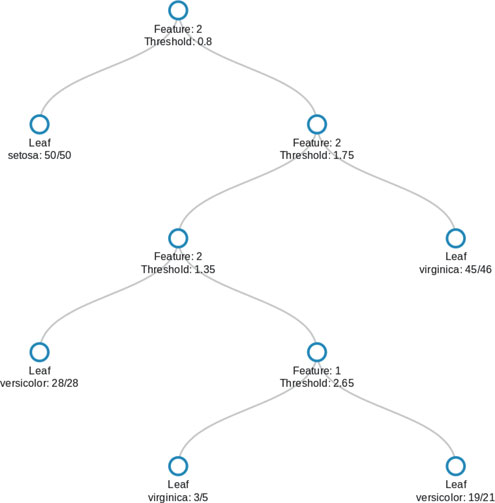
Figure 5.4 Classification tree for the Iris data using only two variables: petal length and petal width.
An alternative way to visualize Figure 5.4 is via a scatterplot with partitions (Figure 5.5). Each one of the five regions shown in Figure 5.5 corresponds to a leaf in the classification tree shown in Figure 5.4.
Recall that a node m represents a region Rm with Nm observations. Again, remaining with the notation of Hastie et al. (2009), the proportion of observations from class g in node m is
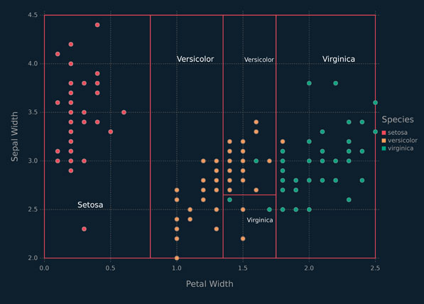
Figure 5.5 Partitioned scatterplot for the iris data.
All observations in node m are classified into the class with the largest proportion of observations; in other words, the majority class:
This is all just a formalization of what is quite clear by inspection of the tree.
Consider how to come up with splits (or splitters) in the first place. One approach is to base them on the misclassification error, i.e.,
Splits can also be based on the Gini index, i.e.,
or the cross-entropy (also called information or deviance), i.e.,
(5.10) |
Note that when used in this way, misclassification error, Gini index, and cross-entropy are referred to as impurity measures. In this vernacular, we want nodes that are as pure as possible. The misclassification error is generally not the impurity measure of choice because it is not differentiable and so less amenable to numerical methods. Accordingly, the Gini index or cross-entropy is typically used.
Now, consider regression trees. They proceed in an analogous fashion to classification trees. However, we now have a regression problem as opposed to a classification problem. The notion of impurity is somewhat more straightforward here and common choices for an impurity measure include the RMSE (5.4) and the MAE (5.5). Splitting requires a little thought. The problem can be formulated as choosing a value v and a variable Xj to split the (training) data into the regions
The choice of j and v is made to minimize some loss function, such as
where is the mean of the (training) observations in Rk, for k = 1, 2. Further splits continue in this fashion.
Consider the following code block. It uses the DecisionTree.jl package to create a regression tree from the food data. The leaves of the tree are merged if the purity of the merged leaf is at least 85%. The resulting regression tree has a depth of 8 and 69 leaves. A tree of this size can be hard to interpret. The DecisionTree.jl package can print out a textual representation of the tree but this leaves much to be desired. At the time of writing, DecisionTree.jl does not support graphical visualizations and plotting a decision tree in Gadfly.jl is not straightforward. We used an unofficial Julia package called D3DecisionTrees.jl to make interactive visualizations of our trees. They render in a web browser and allow the user to click through the nodes and branches to examine subsections of their tree. A static representation of one of these visualizations is used to partially visualize the tree built from the food data (Figure 5.6). Based on an 80-20 train test split of the data, the tree has a test set MAE of 0.82 for predicting student GPA.
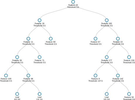
Figure 5.6 Regression tree built from the food data.
using DecisionTree, Random
Random.seed!(35)
## food training data from chapter 3
y = df_food[:gpa]
tmp = convert(Array, df_food[setdiff(names(df_food), [:gpa])])
xmat = convert(Array{Float64}, collect(Missings.replace(tmp, 0)))
names_food = setdiff(names(df_food), [:gpa])
# defaults to regression tree if y is a Float array
model = build_tree(y, xmat)
# prune tree: merge leaves having >= 85% combined purity (default: 100%)
modelp = prune_tree(model, 0.85)
# tree depth is 9
depth(modelp)
# print the tree to depth 3
print_tree(modelp, 3)
#=
Feature 183, Threshold 0.5
L-> Feature 15, Threshold 0.5
L-> Feature 209, Threshold 0.5
L->
R->
R-> Feature 209, Threshold 0.5
L->
R->
R-> Feature 15, Threshold 0.5
L-> Feature 8, Threshold 0.5
L->
R->
R-> Feature 23, Threshold 0.5
L->
R->
=#
# print the variables in the tree
for i in [183, 15, 209, 8, 23]
println("Variable number: ", i, " name: ", names_food[i])
end
#=
Variable number: 183 name: self_perception_wgt3
Variable number: 15 name: cal_day3
Variable number: 209 name: waffle_cal1315
Variable number: 8 name: vitamins
Variable number: 23 name: comfoodr_code11
=#
Trees have lots of advantages. For one, they are very easy to understand and to explain to non-experts. They mimic decision processes, e.g., of a physician perhaps. They are very easy (natural, even) to visualize. However, they are not as good as some other supervised learning methods. Ensembles of trees, however, can lead to markedly improved performance. Bagging, random forests and gradient boosting are relatively well-known approaches for combining trees. However, we need to discuss ensembles and the bootstrap first.
The introduction of the bootstrap by Efron (1979) is one of the single most impactful works in the history of statistics and data science. Use to denote the sample x1,x2, …,xn. Note that, for the purposes of this section, taking xi to be univariate will simplify the explanation. Now, can be considered a set, i.e.,
and is sometime called an ensemble. Suppose we want to construct estimator based upon that sample, and we are interested in the bias and standard error of . A resampling technique can be used, where we draw samples from an ensemble that is itself a sample, e.g., from . There are a variety of resampling techniques available; the most famous of these is called the bootstrap.
Before we look at an illustration of the bootstrap, we need to consider the plug-in principle. Let X1,X2, …,Xn be iid random variables. Note that the cumulative distribution function
defines an empirical distribution. The plug-in estimate of the parameter of interest θF is given by
where is an empirical distribution, e.g., summary statistics are plug-in estimates.
Efron (2002) gives an illustration of the bootstrap very similar to what follows here. Suppose that the data are a random sample from some unknown probability distribution F, θ is the parameter of interest, and we want to know . We can compute , where is the empirical distribution of F, as follows. Suppose we have an ensemble
Sample with replacement from Q, n times, to get a bootstrap sample
and then compute based on . Repeat this process M times to obtain values
based on bootstrap samples
Then,
(5.11) |
where
As M → ∞,
where and are non-parametric bootstrap estimates because they are based on rather than F. Clearly, we want M to be as large as possible, but how large is large enough? There is no concrete answer but experience helps one get a feel for it.
using StatsBase, Random, Statistics
Random.seed!(46)
A1 = [10,27,31,40,46,50,52,104,146]
median(A1)
#46.0
n = length(A1)
m = 100000
theta = zeros(m)
for i = 1:m
theta[i] = median(sample(A1, n, replace=true))
end
mean(theta)
# 45.767
std(theta)
#12.918
## function to compute the bootstrap SE, i.e., an implementation of (5.11)
function boot_se(theta_h)
m = length(theta_h)
c1 = /(1, −(m,1))
c2 = mean(theta_h)
res = map(x −> (x-c2)^2, theta_h)
return(sqrt(*(c1, sum(res))))
end
boot_se(theta)
## 12.918
Now, suppose we want to estimate the bias of given an ensemble . The bootstrap estimate of the bias, using the familiar notation, is
where is computed based the empirical distribution .
## Bootstrap bias
−(mean(theta), median(A1))
#−0.233
In addition to estimating the standard error and the bias, the bootstrap can be used for other purposes, e.g., to estimate confidence intervals. There are a number of ways to do this, and there is a good body of literature around this topic. The most straightforward method is to compute bootstrap percentile intervals.
## 95% bootstrap percentile interval for the median
quantile(theta, [0.025,0.975])
# 2-element Array{Float64,1}:
# 27.0
# 104.0
With the very brief introduction here, we have only scratched the surface of the bootstrap. There are many useful sources for further information on the bootstrap, including the excellent books by Efron and Tibshirani (1993) and Davison and Hinkley (1997).
Consider a regression tree scenario. Now, generate M bootstrap ensembles from the training set and use to denote the regression tree learner trained on the mth bootstrap ensemble. Averaging these predictors gives
This is called bootstrap aggregation, or bagging (Breiman, 1996). Although it seems very simple, bagging tends to result in a better learner than a single tree learner. Note that, with bagging, the M trees are not pruned. Bagging also gives a method for estimating the (test) error, known as the out-of-bag error. When we create a bootstrap ensemble, some observations will be included more than once and some will be left out altogether — the left-out observations are said to be out-of-bag. Typically, around 37% of observations will be out-of-bag for a given tree; to see this, consider that
(5.12) |
is the probability that a single observation is omitted from a bootstrap sample (of size n) and then note how (5.12) behaves as n increases (Figure 5.7).
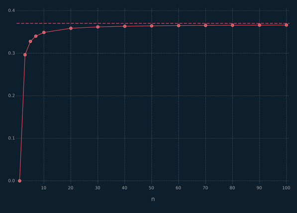
Figure 5.7 Illustration of the value of (5.12) as n increases, with a broken horizontal line at 0.37.
The response for the ith observation can be predicted using the trees for which it was out-of-bag. These can then be averaged to give a prediction for the ith observation. This is sometimes used as an estimate of the test error; however, we will not follow that approach herein.
While bagging can (perhaps greatly) improve regression tree performance, it comes at the expense of the easy visualization and easy interpretability enjoyed by a single regression tree. However, we can evaluate the importance of each predictor variable by considering the extent to which it decreases some cost function, e.g., the RMSE, averaged over all trees. Note that bagging for classification trees proceeds in a very similar fashion to bagging for regression trees. Of course, a different approach is taken to combine the predictions from the M bootstrap samples; this can be done, e.g., via majority vote.
One downside to bagging is that the M trees can be very similar, i.e., they can be highly correlated. The random forests approach (Breiman, 2001a) is an extension of bagging that decorrelates the M trees. For each tree, rather than all predictor variables being available for each split, a random sample of is taken at each split. In fact, a different random sample of predictor variables is considered at each split, for each tree. The result is that the M trees tend to be far more different than for bagging. Sometimes, guidelines such as are used to select M, where p is the total number of predictor variables. We demonstrate a different approach in Section 7.4.2. Note that bagging is a special case of random forests, i.e., with = p, and so it will not be considered separately hereafter. Further material on random forests is deferred to Section 7.4.2, and we continue this chapter with gradient boosting.
Boosting is a general approach to supervised learning, that generates an ensemble with M members from the training set. The ensemble members are generated sequentially, where the current one is created from a base learning algorithm using the residuals from the previous member as the response variable. We will restrict our discussion to decision tree learners. Unlike random forests, boosting does not use bootstrap sampling. It uses the entire dataset, or some subsample thereof, to generate the ensemble. There follows some pseudocode for a straightforward boosting algorithm.
A Straightforward Boosting Algorithm
read in training data X, response Y, M, d, ω
initialize f(x) = 0, e0 = y0
set number of splits per tree to d
for m = 1, 2, …, M
fit tree fm(x) to (X, em−1)
f(x) = f(x) + ωfm(x)
em(x) = em−i(x) − ωfm(x)
end for
return f(x)
The reader is encouraged to reflect on the relationship between this simple pseudocode and (5.1) and (5.2). In the terminology used in Section 5.1, we can think of final error as
Note that ω is a parameter that controls the learning rate, i.e., a small number, and d is the tree depth. Of course, there is a tradeoff between the respective values of ω, d, and M.
Towards the end of Section 5.1, we concluded that we need to move away from thinking only about an error and consider an error together with some way to prevent or mitigate overfitting. The role of ω in the simple boosting algorithm already described is precisely to reduce overfitting. The XGBoost.jl package in Julia is an implementation of extreme gradient boosting (XGBoost), which is based on the idea of a gradient boosting machine (Friedman, 2001). A nice description of XGBoost is given in Chen and Guestrin (2016), where the starting point is a high-level description of the learning problem as the minimization of
In the very simple boosting algorithm described above, the regularization term is not present (Chen and Guestrin, 2016). It is an innovative feature of the XGBoost model which penalizes the model complexity beyond the traditional shrinkage parameter represented above by ω and can greatly improve predictive performance. Given the added complexity, the clearest way to explain XGBoost is by example, as follows.
The first code block has functions used to do 5-fold cross-validation for the boosting learners. The function tunegrid_xgb() creates a grid of the learning rate η and tree depth values d that the classification learners will be trained on. Including values for the number of boosting iterations (rounds) M performed could be a valuable addition to the tuning grid. We set this parameter value to 1000 for ease of exposition. The parameter η is a specific implementation of ω described above. Users of R may be familiar with the gbm package (Ridgeway, 2017), which also performs gradient boosting. The shrinkage parameter of the gbm() function from this package is another implementation of ω. The function binomial_dev() calculates the binomial deviance (5.8), which is used to train the learners, and binary_mcr() calculates the misclassification rate for the labeled outcomes. Note that we are using the MLBase.jl infrastructure to do the cross-validation of our boosting learners. It contains a general set of functions to train any supervised learning model using a variety of re-sampling schemes and evaluation metrics. The cvERR_xgb() function is used by cross_validate() from MLBase.jl to return the error metric of choice for each re-sample iteration being done. The cvResult_xgb() is the master control function for our cross-validation scheme, it uses the MLBase.jl functions cross_validate() and StratifiedKfold() to do stratified cross-validation on the outcome. The cross-validation indices are passed to XGBoost so it can make the predictions and the error metric results are summarized and returned as an array.
## CV functions for classification
using Statistics, StatsBase
## Array of parameters to train models on
## Includes two columns for the error mean and sd
function tunegrid_xgb(eta, maxdepth)
n_eta = size(eta)[1]
md = collect(1:maxdepth)
n_md = size(md)[1]
## 2 cols to store the CV results
res = zeros(*(maxdepth, n_eta), 4)
n_res = size(res)[1]
## populate the res matrix with the tuning parameters
res[:,1] = repeat(md, inner = Int64(/(n_res, n_md)))
res[:,2] = repeat(eta, outer = Int64(/(n_res, n_eta)))
return(res)
end
## MCR
function binary_mcr(yp, ya; trace = false)
yl = Array{Int8}(yp .> 0.5)
disagree = Array{Int8}(ya .!= yl)
mcr = mean(disagree)
if trace
#print(countmap(yl))
println("yl: ", yl[1:4])
println("ya: ", ya[1:4])
println("disagree: ", disagree[1:4])
println("mcr: ", mcr)
end
return(mcr)
end
## Used by binomial_dev
## works element wise on vectors
function bd_helper(yp, ya)
e_const = 1e-16
pneg_const = 1.0 - yp
if yp < e_const
res = +(*(ya, log(e_const)), *(-(1.0, ya), log(-(1.0, e_const))))
elseif pneg_const < e_const
res = +(*(ya, log(-(1.0, e_const))), *(-(1.0, ya), log(e_const)))
else
res = +(*(ya, log(yp)), *(-(1.0, ya), log(pneg_const)))
end
return res
end
## Binomial Deviance
function binomial_dev(yp, ya) #::Vector{T}) where {T <: Number}
res = map(bd_helper, yp, ya)
dev = *(-2, sum(res))
return(dev)
end
## functions used with MLBase.jl
function cvERR_xgb(model, Xtst, Ytst, error_fun; trace = false)
y_p = XGBoost.predict(model, Xtst)
if(trace)
println("cvERR: y_p[1:5] ", y_p[1:5])
println("cvERR: Ytst[1:5] ", Ytst[1:5])
println("cvERR: error_fun(y_p, Ytst) ", error_fun(y_p, Ytst))
end
return(error_fun(y_p, Ytst))
end
function cvResult_xgb(Xmat, Yvec, cvparam, tunegrid; k = 5, n = 50,
trace = false)
result = deepcopy(tunegrid) ## tunegrid could have two columns on input
n_tg = size(result)[1]
## k-Fold CV for each combination of parameters
for i = 1:n_tg
scores = cross_validate(
trind -> xgboost(Xmat[trind,:], 1000, label = Yvec[trind],
param = cvparam, max_depth = Int(tunegrid[i,1]),
eta = tunegrid[i,2]),
(c, trind) -> cvERR_xgb(c, Xmat[trind,:], Yvec[trind],
binomial_dev, trace = true),
## total number of samples
n,
## Stratified CV on the outcome
StratifiedKfold(Yvec, k)
)
if(trace)
println("cvResult_xgb: scores: ", scores)
println("size(scores): ", size(scores))
end
result[i, 3] = mean(scores)
result[i, 4] = std(scores)
end
return(result)
end
The next code block illustrates how the functions detailed in the previous code block can be used to classify beers in the beer data as either lagers or ales. We start by creating an 80-20 training test split of the data, stratified on outcome. Next, there is an array of parameters that we will pass to all of our XGBoost learners. Besides the parameters being used to generate the tuning grid, the others will be held constant across learners. The tunegrid_xgb() function is used to generate a training grid for η and d. Increasing the tree depth and η is one way to increase the complexity of the XGBoost learner. The cvResult_xgb() function is used to generate the training results illustrated in Figure 5.8, which suggest that learners with small η values and medium sized trees are classifying the beers best.
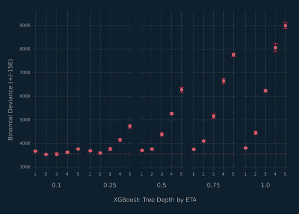
Figure 5.8 Summary of cross-validation performance for XGBoost from 5-fold cross-validation.
The horizontal line in Figure 5.8 is one standard error above the smallest cross-validation training deviance. Because there are a number of learners with error bars overlapping the line, we use the one-standard error method for choosing the final learner. This method was first proposed by Breiman et al. (1984) in the context of classification and regression trees and is discussed further by Hastie et al. (2009). The method finds the simplest, i.e., most regularized, learner configuration within one standard error above the numerically best learner, i.e., the configuration with the lowest error rate. The results are depicted in Figure 5.9. We choose the learner with η = 0.1 and a tree depth of 2. This learner is run on the test set data and has a misclassification rate of 8.2% and a deviance of 4458.08. As expected, the deviance is larger than the value found by cross-validation but still very reasonable.
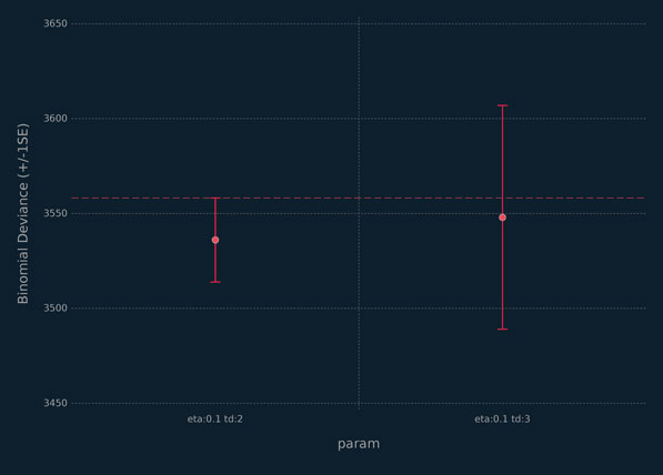
Figure 5.9 Summary of results for the 1 SE method applied to the XGBoost analysis of the beer data.
## 80/20 split
splt = 0.8
y_1_ind = N_array[df_recipe[:y] .== 1]
y_0_ind = N_array[df_recipe[:y] .== 0]
tr_index = sort(
vcat(
sample(y_1_ind, Int64(floor(*(N_y_1, splt))), replace = false),
sample(y_0_ind, Int64(floor(*(N_y_0, splt))), replace = false)
)
)
tst_index = setdiff(N_array, tr_index)
df_train = df_recipe[tr_index, :]
df_test = df_recipe[tst_index, :]
## Check proportions
println("train: n y: $(sum(df_train[:y]))")
println("train: % y: $(mean(df_train[:y]))")
println("test: n y: $(sum(df_test[:y]))")
println("test: % y: $(mean(df_test[:y]))")
## Static boosting parameters
param_cv = [
"silent" => 1,
"verbose" => 0,
"booster" => "gbtree",
"objective" => "binary:logistic",
"save_period" => 0,
"subsample" => 0.75,
"colsample_bytree" => 0.75,
"alpha" => 0,
"lambda" => 1,
"gamma" => 0
]
## training data: predictors are sparse matrix
tmp = convert(Array, df_train[setdiff(names(df_train), [:y])])
xmat_tr = convert(SparseMatrixCSC{Float64,Int64},
collect(Missings.replace(tmp, 0)))
## CV Results
## eta shrinks the feature weights to help prevent overfilling by making
## the boosting process more conservative
## max_depth is the maximum depth of a tree; increasing this value makes
## the boosting process more complex
tunegrid = tunegrid_xgb([0.1, 0.25, 0.5, 0.75, 1], 5)
N_tr = size(xmat_tr)[1]
cv_res = cvResult_xgb(xmat_tr, y_tr, param_cv, tunegrid,
k = 5, n = N_tr, trace = true)
## dataframe for plotting
cv_df = DataFrame(tree_depth = cv_res[:, 1],
eta = cv_res[:, 2],
mean_error = cv_res[:, 3],
sd_error = cv_res[:, 4],
)
cv_df[:se_error] = map(x -> x / sqrt(5), cv_df[:sd_error])
cv_df[:mean_min] = map(-, cv_df[:mean_error], cv_df[:se_error])
cv_df[:mean_max] = map(+, cv_df[:mean_error], cv_df[:se_error])
## configurations within 1 se
min_dev = minimum(cv_df[:mean_error])
min_err = filter(row -> row[:mean_error] == min_dev, cv_df)
one_se = min_err[1, :mean_max]
possible_models = filter(row -> row[:mean_error] <= one_se, cv_df)
#####
## Test Set Predictions
tst_results = DataFrame(
eta = Float64[],
tree_depth = Int64[],
mcr = Float64[],
dev = Float64[])
## using model configuration selected above
pred_tmp = XGBoost.predict(xgboost(xmat_tr, 1000, label = y_tr,
param = param_cv, eta =0.1, max_depth = 2), xmat_tst)
tmp = [0.1, 2, binary_mcr(pred_tmp, y_tst), binomial_dev(pred_tmp, y_tst)]
push!(tst_results, tmp)
#####
## Variable importance from the overall data
fit_oa = xgboost(xmat_oa, 1000, label = y_oa, param = param_cv, eta = 0.1,
max_depth = 2)
## names of features
names_oa = map(string, setdiff(names(df_recipe), [:y]))
fit_oa_imp = importance(fit_oa, names_oa)
## DF for plotting
N_fi = length(fit_oa_imp)
imp_df = DataFrame(fname = String[], gain = Float64[], cover = Float64[])
for i = 1:N_fi
tmp = [fit_oa_imp[i].fname, fit_oa_imp[i].gain, fit_oa_imp[i].cover]
push!(imp_df, tmp)
end
sort!(imp_df, :gain, rev=true)
The learner chosen by the one-standard error method is run on the full data to determine which variables are most predictive of the beer types. We use the full dataset because the important variables could differ from those found in the training set. The results are displayed graphically in Figure 5.10.
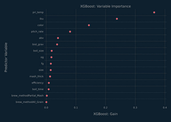
Figure 5.10 Variable importance plot from the XGBoost analysis of the beer data.
XGBoost measures variable importance in a number of ways, we will focus on the gain measure. It is the mean accuracy improvement brought on by creating a split in a tree on this variable across the boosting ensemble. The gain is scaled to be between 0 and 1. There are three important predictor variables for the beer data: primary brewing temperature; IBU; and colour units. This makes sense considering that it is well-known that ales are brewed at higher temperatures and tend have a higher bitterness rating (Oliver and Colicchio, 2011). Ales include many dark-coloured beers, which might account for the predictive ability of the colour variable.
The following code block details how we went about training XGBoost regression learners on the food data. We have many of the same functions but with slightly different configurations. The tunegrid_xgb_reg() function adds a third parameter to the tuning grid, but it is otherwise the same as the one we used for the classification learners. The XGBoost models are run for 1000 iterations. The error metrics have changed: now, they are the MAE, calculated using medae(), and the RMSE, calculated using rmse(). Note that cvResult_xgb_reg() plays an analogous role to cvResult_xgb(), controlling the cross-validation process. Specifically, it carries out unstratified cross-validation and trains the learners using the medae() function.
## CV Functions for Regression
function tunegrid_xgb_reg(eta, maxdepth, alpha)
n_eta = size(eta)[1]
md = collect(1:maxdepth)
n_md = size(md)[1]
n_a = size(alpha)[1]
## 2 cols to store the CV results
res = zeros(*(maxdepth, n_eta, n_a), 5)
n_res = size(res)[1]
println("N:", n_res, " e: ", n_eta, " m: ", n_md, " a: ", n_a)
## populate the res matrix with the tuning parameters
n_md_i = Int64(/(n_res, n_md))
res[:,1] = repeat(md, outer=n_md_i)
res[:,2] = repeat(eta, inner = Int64(/(n_res, n_eta)))
res[:,3] = repeat(repeach(alpha, (n_md)), outer=n_a)
return(res)
end
function medae(yp, ya)
## element wise operations
res = map(yp, ya) do x,y
dif = -(x, y)
return(abs(dif))
end
return(median(res))
end
function rmse(yp, ya)
## element wise operations
res = map(yp, ya) do x,y
dif = -(x, y)
return(dif^2)
end
return(sqrt(mean(res)))
end
function cvResult_xgb_reg(Xmat, Yvec, cvparam, tunegrid; k = 5, n = 50,
trace = false)
result = deepcopy(tunegrid)
n_tg = size(result)[1]
## k-Fold CV for each combination of parameters
for i = 1:n_tg
scores = cross_validate(
## num_round investigate
trind -> xgboost(Xmat[trind,:], 1000, label = Yvec[trind],
param = cvparam, max_depth = Int(tunegrid[i,1]),
eta = tunegrid[i,2], alpha = tunegrid[i,3]),
(c, trind) -> cvERR_xgb(c, Xmat[trind,:], Yvec[trind], medae,
trace = true),
n, ## total number of samples
Kfold(n, k)
)
if(trace)
println("cvResult_xgb_reg: scores: ", scores)
println("size(scores): ", size(scores))
end
result[i, 4] = mean(scores)
result[i, 5] = std(scores)
end
return(result)
end
The following code block illustrates how the functions defined above can be used to train our XGBoost regression learners. Start by making a 80-20 training-test split of the data. Then define the static boosting parameters for the XGBoost learners. The tuning grid is generated for values of η, d, and α, an L1 regularization term on the learner weights. The α parameter is one of XGBoost’s regularization terms and, when included in the model tuning, can produce very predictive and fast models when there are a large number of predictor variables. The 5-fold cross-validation results are stored in the cv_res_reg array and visualized in Figure 5.11. Once again, there are many candidate learners to choose from. Learners with larger tree depths and smaller values of η and α seem to perform best on the training set.
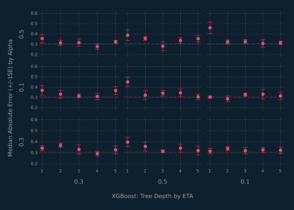
Figure 5.11 Summary of results for 5-fold cross-validation from the XGBoost analysis of the food data.
## 80/20 train test split
splt = 0.8
tr_index = sample(N_array, Int64(floor(*(N, splt))), replace = false)
tst_index = setdiff(N_array, tr_index)
df_train = df_food[tr_index, :]
df_test = df_food[tst_index, :]
## train data: predictors are sparse matrix
y_tr = convert(Array{Float64}, df_train[:gpa])
tmp = convert(Array, df_train[setdiff(names(df_train), [:gpa])])
xmat_tr = convert(SparseMatrixCSC{Float64,Int64},
collect(Missings.replace(tmp, 0)))
## Static boosting parameters
param_cv_reg = [
"silent" => 1,
"verbose" => 0,
"booster" => "gbtree",
"objective" => "reg:linear",
"save_period" => 0,
"subsample" => 0.75,
"colsample_bytree" => 0.75,
"lambda" => 1,
"gamma" => 0
]
## CV Results
## eta shrinks the feature weights to help prevent overfilling by making
## the boosting process more conservative
## max_depth is the maximum depth of a tree; increasing this value makes
## the boosting process more complex
## alpha is an L1 regularization term on the weights; increasing this value
## makes the boosting process more conservative
tunegrid = tunegrid_xgb_reg([0.1, 0.3, 0.5], 5, [0.1, 0.3, 0.5])
N_tr = size(xmat_tr)[1]
cv_res_reg = cvResult_xgb_reg(xmat_tr, y_tr, param_cv_reg, tunegrid,
k = 5, n = N_tr, trace = true)
## add the standard error
cv_res_reg = hcat(cv_res_reg, ./(cv_res_reg[:,5], sqrt(5)))
## dataframe for plotting
cv_df_r = DataFrame(tree_depth = cv_res_reg[:, 1],
eta = cv_res_reg[:, 2],
alpha = cv_res_reg[:, 3],
medae = cv_res_reg[:, 4],
medae_sd = cv_res_reg[:, 5]
)
cv_df_r[:medae_se] = map(x -> /(x, sqrt(5)), cv_df_r[:medae_sd])
cv_df_r[:medae_min] = map(-, cv_df_r[:medae], cv_df_r[:medae_se])
cv_df_r[:medae_max] = map(+, cv_df_r[:medae], cv_df_r[:medae_se])
min_medae = minimum(cv_df_r[:medae])
min_err = filter(row -> row[:medae] == min_medae, cv_df_r)
one_se = min_err[1, :medae_max]
#######
## Test Set Predictions
tst_results = DataFrame(
eta = Float64[],
alpha = Float64[],
tree_depth = Int64[],
medae = Float64[],
rmse = Float64[])
## using configuration chosen above
pred_tmp = XGBoost.predict(xgboost(xmat_tr, 1000, label = y_tr,
param = param_cv_reg, eta =0.1, max_depth = 1, alpha = 0.1), xmat_tst)
tmp = [0.1, 0.1, 1, medae(pred_tmp, y_tst), rmse(pred_tmp, y_tst)]
push!(tst_results, tmp)
#####
## Variable Importance from the overall data
fit_oa = xgboost(xmat_oa, 1000, label = y_oa, param = param_cv_reg,
eta = 0.1, max_depth = 1, alpha = 0.1)
## names of features
# names_oa = convert(Array{String,1}, names(df_food))
names_oa = map(string, setdiff(names(df_train), [:gpa]))
fit_oa_imp = importance(fit_oa, names_oa)
## DF for plotting
N_fi = length(fit_oa_imp)
imp_df = DataFrame(fname = String[], gain = Float64[], cover = Float64[])
for i = 1:N_fi
tmp = [fit_oa_imp[i].fname, fit_oa_imp[i].gain, fit_oa_imp[i].cover]
push!(imp_df, tmp)
end
sort!(imp_df, :gain, rev=true)
Given the plethora of candidate learners, we again apply the one-standard error method to select the best candidate learner parameter configuration. The results are summarized in Figure 5.12. There are six candidates to choose from. We opt for the stump learner with η = α = 0.1 and d = 1, because it has the most regularization and the simplest tree structure. When run on the test set, the MAE is 0.533 and the RMSE is 0.634.
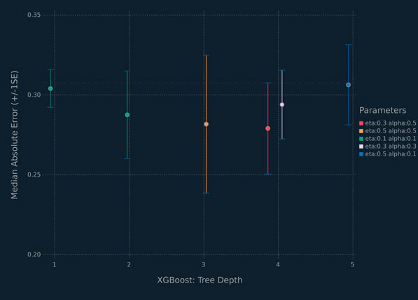
Figure 5.12 Summary of results for the 1 SE method applied to the XGBoost analysis of the food data.
This learner was used to determine the variable importance on the overall data. The results are displayed in Figure 5.13. The left-hand panel contains a violin plot of the overall gain scores. It is obvious that most of the predictor variables have little-to-no effect on the prediction of student GPA. There are many weak predictor variables that play a part in successfully predicting student GPA from these data. Based on the variable importance plot in Figure 5.13, the important predictor variables in the learner reflect: a highly educated father; a poorly educated mother; being able to estimate the calories in food; and measuring one’s body weight.
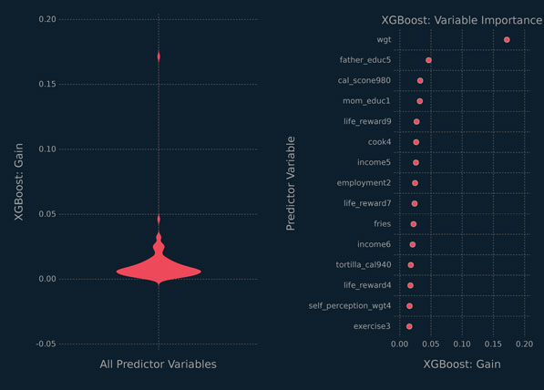
Figure 5.13 Violin plot and variable importance plot from the XGBoost analysis of the food data.
Selected supervised learning techniques have been covered, along with Julia code needed for implementation. The primary goal of this book is to expose the reader to Julia and, as mentioned in the Preface, it is not intended as a thorough introduction to data science. Certainly, this chapter cannot be considered a thorough introduction to supervised learning. Some of the more notable absentees include generalized additive models, neural networks, and their many extensions as well as assessment tools such as sensitivity, specificity, and receiver operating characteristic (ROC) curves. Random forests were discussed in this chapter; however, their implementation and demonstration is held over for Section 7.4.2.
The idea that some learners are more prone to overfitting than others was touched upon in Section 5.1. This is a topic that deserves careful thought. For example, we applied the one standard error rule to reduce the complexity when fitting our kNN learner, by choosing the smallest k when several values gave similar performance. The reader may be interested to contrast the use of gradient boosting in Section 5.7 with that of random forests (Section 7.4.2). It is, perhaps, difficult to escape the feeling that an explicit penalty for overfitting might benefit random forests and some other supervised learning approaches that do not typically use one. When using random forests for supervised learning, it is well known that increasing the size of the forest does not lead to over-fitting (Hastie et al., 2009, Chp. 15). When using it for regression, utilizing unpruned trees in the forest can lead to over-fitting which will increase the variance of the predictions (Hastie et al., 2009, Chp. 15). Despite this, few software packages provide this parameter for performance tuning.