CHAPTER NINE
Interest Rate and Reinvestment Risks
Bond portfolios can be divided into two categories:
- Portfolios where the investor reinvests
- Portfolios where the investor distributes (lives on) the interest
If the investor is living on the income, the goal is to maximize the portfolio’s long-term current return. For a portfolio where the investor reinvests the cash flows, managing interest rate risk becomes a more complex exercise.
When the interest payments are being reinvested, the total return in dollars (T$R) that you earn from owning a bond or bond portfolio is the sum of the three components of return that a bond offers, namely:
T$R = MV + I + IOI
Where:
- Market Value (MV) is the current market value of the bond, which can be more or less than par and will fluctuate with changes in interest rates and credit quality.
- Interest (I) is the total interest that the portfolio has paid since you bought the bond.
- Interest on Interest (IOI) is the amount of interest you earn by reinvesting the interest payments (as well as any principal payments) you receive. This is the component of return that investors too often overlook despite the fact that it is sometimes the largest of the three components of the total return.
Every change in market interest rates impacts two components of the T$R—the MV of the bond and the IOI. If interest rates rise, the market value of the bond declines, but the amount of interest on interest that the investor earns rises.
The MV declines because, as interest rates rise, the market value of the bond must decline in order to offer a competitive yield to maturity. No one is going to pay full value for a bond that pays 6% if new bonds being issued are offering 8%. The IOI rises because as market interest rates rise, the rate at which the interest payments that are received can be reinvested also increases. If interest rates decline, the reverse happens and the MV rises, while the amount of IOI that the investor can expect to earn declines. Thus, any change in rates has a yin-yang impact on MV and IOI.
While any change in market interest rates will cause a change in the MV and IOI, a change in market interest rates does not impact both components of return to the same degree over the same time frame. Let’s look at the change in MV and IOI in greater detail—starting first with the impact of a change in interest rates on the bond’s market value.
INTEREST RATE IMPACT ON MARKET VALUE
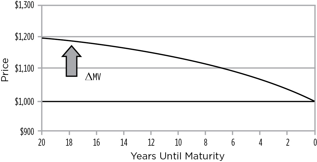
When interest rates change, the market value of bonds reacts immediately. As time passes, however, the change in market value that results from a change in interest rates—either positive or negative—is mitigated because the bond accretes toward par. Thus, the change in a bond’s market value (ΔMV) is maximized immediately after market interest rates change—and is mitigated by the passage of time. At maturity, any loss or gain is eliminated because the bond matures at par, as shown in Figure 9.1.
FIGURE 9.1
Change in MV vs. Time Resulting from an Instantaneous Rise in Rates from 10% to 12% on a Bond with a 10% Coupon

Likewise, when interest rates decline, the bond’s MV rises immediately—but this rise is also mitigated by the passage of time, as shown in Figure 9.2. At maturity, any gain stemming from a decline in rates is lost because the bond matures at par.
Change in Market Value vs. Time from a Single Instantaneous Decline in Market Interest Rates
INTEREST RATE IMPACT ON INTEREST ON INTEREST
A change in market interest rates has the opposite effect on the change in the amount interest on interest ΔIOI. Unlike the change in market value that happens immediately and gets smaller as time passes, the ΔIOI happens slowly and becomes larger as time passes.
You only start to earn interest on interest after you receive your first interest payment. The difference between the amount of IOI that you originally expected to earn and the amount of IOI that is earned after rates rise is the ΔIOI. As time passes, you receive and reinvest more interest payments, and the magnitude of the ΔIOI increases. The ΔIOI increases as time passes and reaches its maximum value at maturity, as shown in Figure 9.3. Figure 9.4 summarizes the relationship between ΔMV and ΔIOI.
IOI for a 20-Year 10% Bond Assuming 8%, 10%, and 12% Reinvestment Rates
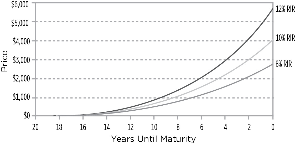
FIGURE 9.4
Summarizing the ΔMV vs. the ΔIOI
|
Change |
Maximum Value |
Passage of Time |
|
ΔMV |
Immediately |
Mitigates |
|
ΔIOI |
At Maturity |
Exacerbates |
It should be obvious that, over a short investment horizon, ΔMV will be greater than ΔIOI. Since the ΔMV lowers your T$R when rates rise, over a short time frame your actual total dollar return (T$RACT) declines relative to the T$R you originally expected (T$REXP) if market interest rates remain unchanged. In other words, in a rising rate environment, your T$RACT is lower than your T$REXP—provided your investment horizon is short. However, as your investment horizon increases, any negative impact of ΔMV decreases and any positive impact of ΔIOI increases. Since, as time passes, the ΔIOI increases and the ΔMV decreases, eventually your T$RACT will be greater than T$REXP. Thus, given a long enough time frame, you actually benefit from a rise in market interest rates.
It stands to reason that, if over a short-term time horizon, the T$RACT is less than T$REXP, and if, over a long time horizon, the T$RACT is greater than T$REXP, there must be some point along the bond’s life where the T$RACT equals T$REXP despite a change in market interest rates. This point is defined as the bond’s duration point. Since at the duration point the change in interest rates has no impact on the investor’s T$R, the bond effectively hedges itself at its duration point. Thus, at the duration point the investor earns the YTM the investor originally expected, despite the subsequent change in market interest rates, as shown in Figure 9.5.
FIGURE 9.5
ΔMV vs. ΔIOI over Time
|
Pre-duration |
ΔMV > ΔIOI |
T$RACT < T$REXP |
|
Duration |
ΔMV = ΔIOI |
T$RACT = T$REXP |
|
Post-duration |
ΔMV < ΔIOI |
T$RACT > T$REXP |
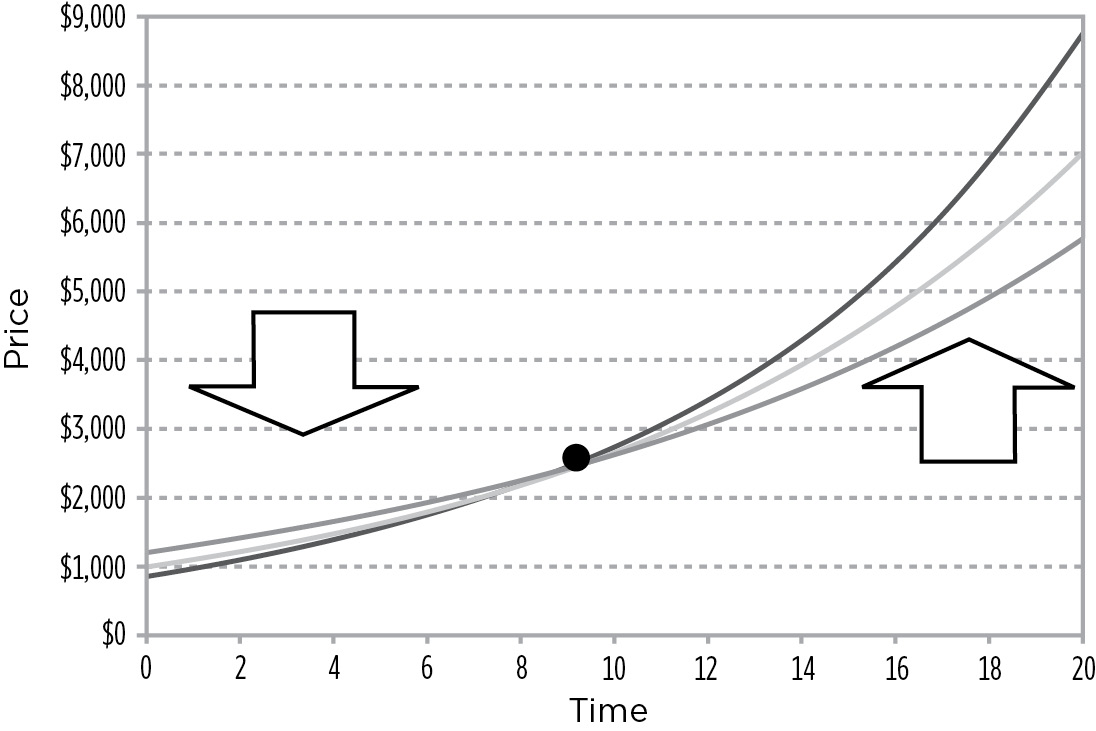
If we were to graph the T$R of a 10% 20-year bond and assume that rates fall to 8% and rise to 12%, the curves would look like the ones illustrated in Figure 9.6.
T$R of a 10% 20-Year Bond Assuming 2% Rate Changes
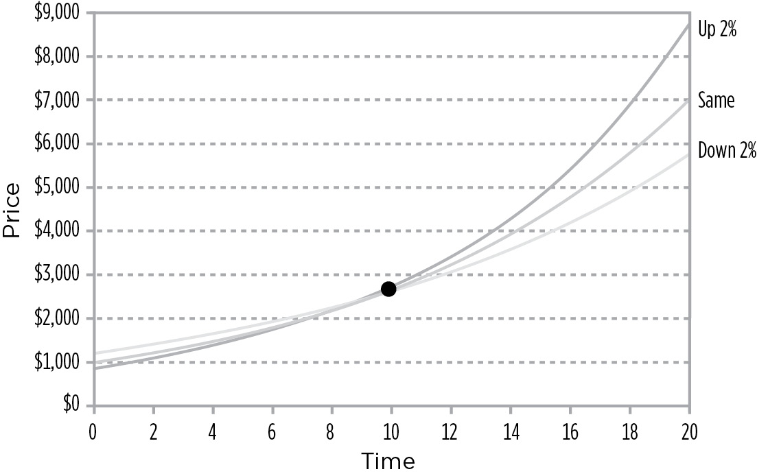
Investors have to be realistic about their level of patience. If interest rates go up, bond prices fall, and investors have a tendency to panic and sell. One key to being a successful investor is being able to stay the course. Duration tells investors how much patience they will need. As shown in Figure 9.6, if rates rise, it will take an investor 9 years of reinvesting at the higher rate for the portfolio to catch up with its original projected value. Does the investor have 9 years of patience? If not, the investor should shorten the portfolio to the point where they are comfortable. If an investor is only willing to wait 3 years to catch up with its original projected value, the investor should have a portfolio that has a duration of 3 years.
This brings us to the second definition of duration: Duration is the point along a bond’s life where risk is minimized.
In most strategic asset allocation models, we define risk as the uncertainty of return and measure it by calculating the standard deviation of the portfolio. If risk is defined this way, then a bond has the least degree of risk if it is held to its duration point. The further the holding period or investment horizon deviates from the bond’s duration—in either direction—the greater the uncertainty of return and, therefore, the greater the risk.
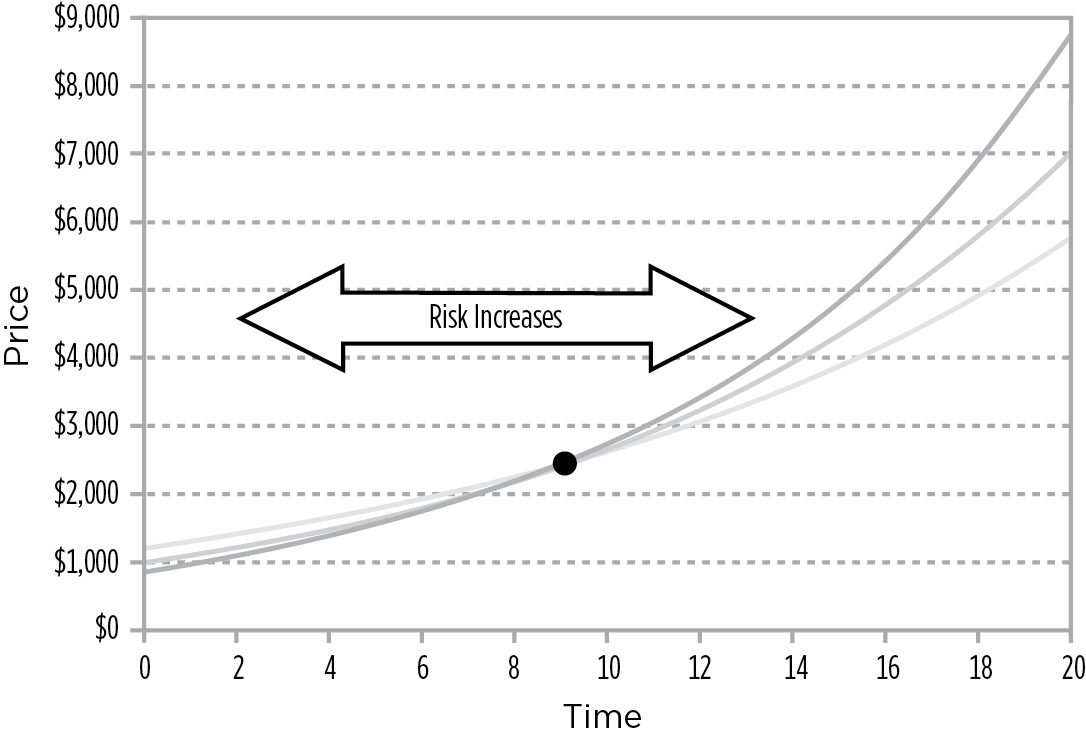
Conversely, traders who hold bonds for very short periods of time and investors who hold bonds until they mature have the greatest degree of uncertainty with regards to their return. At these extremely short and long time investment horizons, interest rate risk and reinvestment risk have no opportunity to offset each other—and risk is maximized, as Figure 9.7 shows.
FIGURE 9.7
T$R of a 10% 20-Year Bond Assuming 2% Rate Changes
Following this same line of logic leads us to the third definition of duration: Duration is the point in a bond’s life where an investor who reinvests actually earns the bond’s YTM.
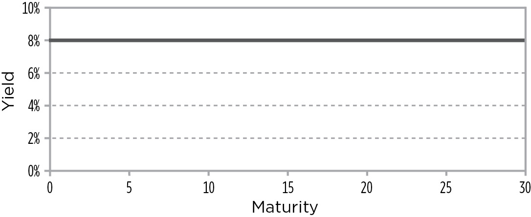
For investors who reinvest, the YTM isn’t the return they’ll earn if the bond is held to maturity. The reason is that each interest payment that is received is reinvested—and the rate at which it will be reinvested is dependent upon interest rate changes during the time the investor owns the bond. Figure 9.8 shows the assumed shape of the yield curve.
FIGURE 9.8
Assumed Shape of the Yield Curve in the YTM Calculation of a Bond Offering an 8% YTM
The only point in a bond’s life when an investor can reasonably anticipate earning the YTM is if the investor holds the bond to its duration point. Figure 9.9 shows the YTM for reinvestors at duration and at maturity.
YTM at Duration and Maturity
The reason an investor earns the YTM at the duration point and the reason why the ΔMV and the ΔIOI offset each other at the duration point provides the 4th definition of duration: Duration is the point in a bond’s life where an investor receives half of the present value of the bond’s future cash flows.
Consider that for reinvestors the duration point is both:
- The point where the two risks (interest rate risk and reinvestment risk) balance
- The point where reinvestors actually earn the YTM.
Now, it makes sense that the duration point would be the point in a bond’s life where an investor receives half of the present value the bond’s future cash flows—with the second half still to come.
In order to calculate where this point is, we need to review two concepts:
Time-Weighting Future Cash Flows
Starting with time-weighting, consider the following two cash flows:
Payable in 1 year(s): $100
Payable in 2 year(s): $100
If you want to determine when (on average) monies are received, time-weight the cash flows by the times when they are received:
1 × $100 = $100
2 × $100 = $200
Total (unweighted) = $200
Total (time-weighted) = $300
$300 Total Time-Weighted Cash Flows
$200 Total Cash Flows
Now, reduce the equation and eliminate cash flow from both the numerator and denominator:
$300 / $200 = 1.5 years
In other words, reinvestors receive their money (on average) in 1.5 years.
Now, consider these three cash flows:
Payable in 1 year(s): $100
Payable in 2 year(s): $100
Payable in 3 year(s): $100
ANSWER:
To determine when (on average) reinvestors receive their money, time-weight the cash flows as follows:
1 × $100 = $100
2 × $100 = $200
3 × $100 = $300
Total cash flows = $300
Total time-weighted cash flows = $600
$600 Total Time-Weighted Cash Flows
$300 Total Cash Flows
$600 / $300 = 2 years
In other words, reinvestors receive their money (on average) in 2 years.
PROBLEM 9B
Now, consider these next three unequal cash flows:
Payable in 1 year(s): $300
Payable in 2 year(s): $100
Payable in 3 year(s): $600
To determine when (on average) reinvestors receive their money, time-weight the cash flows as follows:
1 × $300 = $300
2 × $100 = $200
3 × $600 = $1,800
Total (unweighted) = $1,000
Total (time-weighted) = $2,300
$2,300 Total Time-Weighted Cash Flows
$1,000 Total Cash Flows
$2,300 / $1,000 = 2.3 years
Even though they receive the money over 3 years, since the bulk of it comes at the end of the third year, on average reinvestors receive it in 2.3 years.
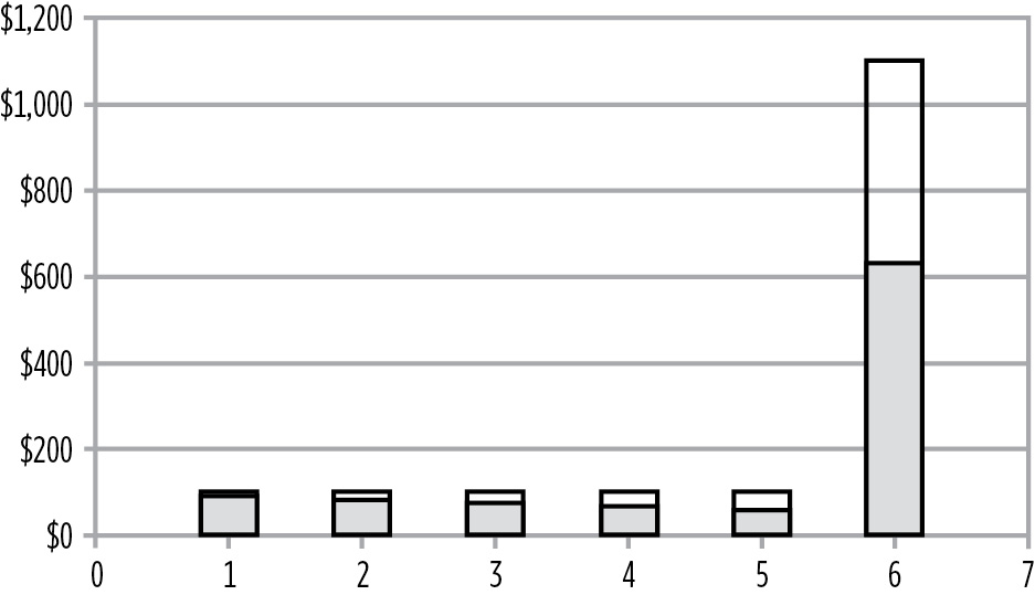
PROBLEM 9C
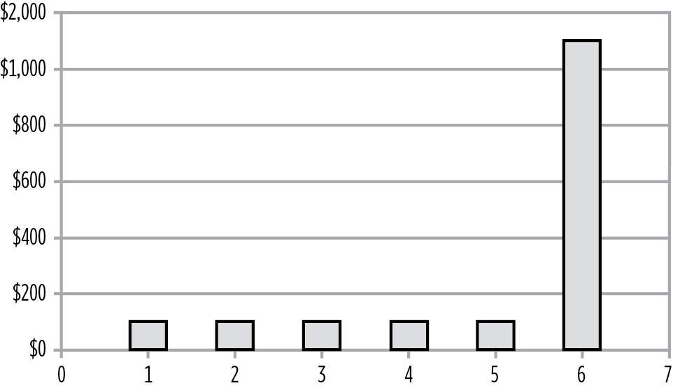
Consider the cash flow schedule of the 10% 6-year eurobond shown in Figure 9. 10. (Note: Eurobonds only pay interest once per year.)
Payable in 1 year(s): $100
Payable in 2 year(s): $100
Payable in 3 year(s): $100
Payable in 4 year(s): $100
Payable in 5 year(s): $100
Payable in 6 year(s): $1,100
The Cash Flows of a 6% 10-Year Eurobond
Determine when, on average, we receive our money.
ANSWER:
Time-weight the cash flows as follows:
1 × $100 = $100
2 × $100 = $200
3 × $100 = $300
4 × $100 = $400
5 × $100 = $500
6 × $1,100 = $6,600
Total cash flow = $1,600
Total time-weighted cash flow = $8,100
$8,100 Time-Weighted Cash Flows
$1,600 Total Cash Flows
$8,100 / $1,600 = 5.06 years
Time-Discounting Future Cash Flows
Now that we have reviewed time-weighting, let’s turn our attention to discounting. Future cash flows are discounted because a dollar received today is more valuable than a dollar received in the future; a dollar received today can be reinvested. The longer an investor has to wait to receive money, the less valuable it becomes.
For the 6-year 10% eurobond described in Problem 9C and priced at par, the present value of each future cash flow can be found by discounting it by the bond’s YTM. Since the bond is trading at par, its coupon and YTM are the same—that is 10%.
If we discount each cash flow at 10% using the formula depicted in Figure 9.11, then the present values would be as depicted in Figure 9.12 and Figure 9.13.
FIGURE 9.11
PV Formula
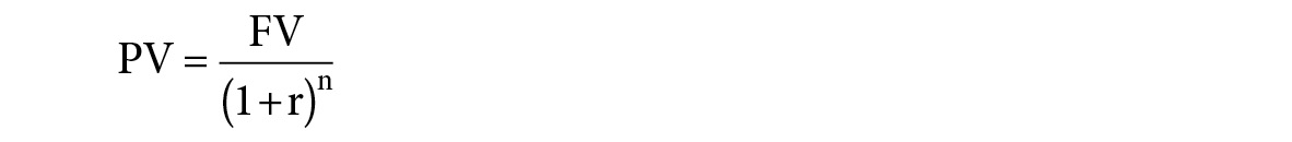
FIGURE 9.12
The Present Values
|
Year |
Cash Flow |
PV |
|
1 |
$100 |
$90.91 |
|
2 |
$100 |
$82.64 |
|
3 |
$100 |
$75.13 |
|
4 |
$100 |
$68.30 |
|
5 |
$100 |
$62.09 |
|
6 |
$1,100 |
$620.92 |
Present Value of the Cash Flows
If we then time-weight the PV of the cash flows, the result is 4.79 years.
|
Year |
Cash Flow |
PV |
Time Weighted |
|
1 |
$100 |
$90.91 |
$90.91 |
|
2 |
$100 |
$82.64 |
$165.29 |
|
3 |
$100 |
$75.13 |
$225.39 |
|
4 |
$100 |
$68.30 |
$273.21 |
|
5 |
$100 |
$62.09 |
$310.46 |
|
6 |
$1,100 |
$620.92 |
$3,725.53 |
|
Totals |
$1,000.00 |
$4,790.79 |
|
Duration = $4,790.79 / $1,000.00 = 4.79 years
In other words, in 4.79 years you will have received half of the bond’s value (adjusted for time) with half still to come, as shown in Figure 9.14.
Balance Point of the Time-Weighted Future Cash Flows

As we defined before, this time-weighted present value of the cash flows is the bond’s duration—often referred to as “Macaulay’s duration.” It is called Macaulay’s duration because Frederick Macaulay was the first person to publish work on duration. It is at the duration point where the various T$R curves intersect.
As some additional illustrative examples, let’s calculate the duration of some bonds:
- An 8% 4-year US Corporate Bond priced at 106½
- A 15-year Treasury zero coupon bond priced to offer a 9% return
- A US Treasury 15%-July-15-2012 as of 3/3/01; assume the bond is priced to offer a 10.45% return
PROBLEM 9D
Calculate the duration of the 8% 4-year US Corporate Bond at 106½.
ANSWER:
Because this bond pays interest semiannually, it generates eight cash flows. To calculate its duration, first calculate duration in periods, and then convert it to duration in years. The discount rate is the YTM per period.
|
Year |
Cash Flow |
PV |
Time Weighted |
|
1 |
40 |
$38.81 |
$38.81 |
|
2 |
40 |
$37.65 |
$75.30 |
|
3 |
40 |
$36.53 |
$109.59 |
|
4 |
40 |
$35.44 |
$141.77 |
|
5 |
40 |
$34.39 |
$171.93 |
|
6 |
40 |
$33.36 |
$200.16 |
|
7 |
40 |
$32.37 |
$226.57 |
|
8 |
1,040 |
$816.46 |
$6,531.65 |
|
$1,065.00 |
$7,495.77 |
$7,495.77 Total Time-Weighted Cash Flow
$1,065.00 Sum of PV of Cash Flows
$7,495.77 / $1,065.00 = 7.038 Duration in periods
To convert duration in periods to duration in years, which is how duration is typically expressed, divide the duration in periods by the number of periods per year. In this problem:
Duration in years = 7.038 / 2 payments per year = 3.519
Alternatively, the same duration can be calculated using the duration function in Excel.
To use the duration function in Excel, first make sure that the Analysis ToolPak is activated. To do so, simply check Analysis ToolPak, which can be found under Tools > Add-Ins. Then, in any cell, paste the function by selecting Insert > Function > Financial > Duration. This brings up the dialog box shown in Figure 9.15.
FIGURE 9.15
Microsoft Excel Duration Function Dialog Box
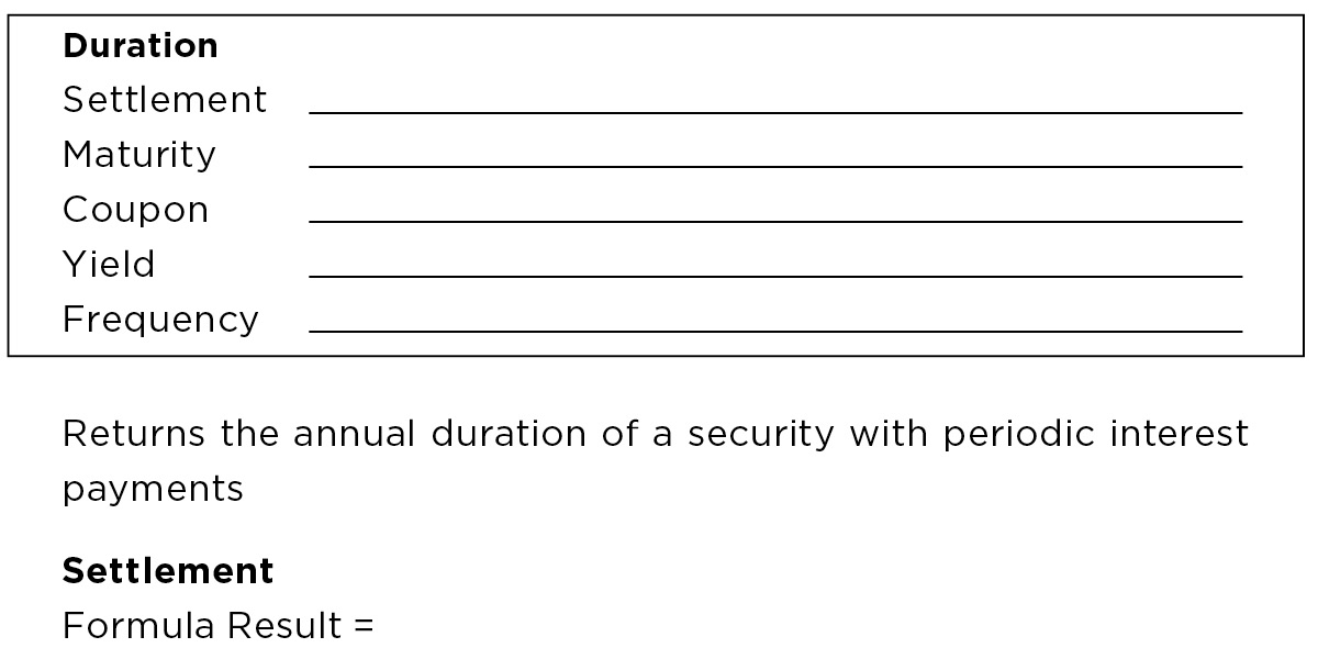
In the Settlement text box, enter the settlement date inside a set of quotation marks: “MM/DD/YYYY”. Alternatively, enter address of the cell that contains the settlement date or the current date, if the bond is already owned.
In the Maturity text box, enter the maturity date inside a set of quotation marks “MM/DD/YYYY” or enter the address of the cell that contains the maturity date.
In the Coupon text box, enter the bond’s annual coupon. (A 7.25% coupon would be entered as .0725.) Alternatively, you can enter the address of the cell that contains the coupon.
In the Yield text box, enter the current YTM to at least two decimal places. (A YTM of 11.33% would be entered as .1133.) Alternatively, you can enter the address of the cell that contains the coupon.
In the Frequency text box, enter the number of periods per year, typically 1 for eurobonds and 2 for US bonds.
Scroll down to the last text box: Calendar basis. For all US bonds except Treasuries enter 0—which means a 30/360 calendar. For Treasuries enter 1. When you are finished, click OK to save the settings and close the dialog box.
The duration is then displayed in the cell. Click the boxed question mark if you have any questions. Clicking this question mark brings up the Help screens.
PROBLEM 9E
Calculate the duration of a 15-year Treasury zero coupon bond priced to offer a 9% return.
ANSWER:
Since this is a zero coupon bond, there is only one cash flow. Even though there is only one cash flow, the convention is still to calculate and express the yield as if the bond compounds semiannually. Thus, the table we use to calculate duration would be as shown in Figure 9.16.
FIGURE 9.16
Cash Flow Table for Zero Coupon Bond
|
Number |
Cash Flow |
PV |
Time Weighted |
|
1 |
0 |
$0.00 |
$0 |
|
2-29 |
0 |
$0.00 |
$0 |
|
30 |
1,000 |
$267.00 |
$8,010 |
|
Totals |
$267.00 |
$8,010 |
|
Time-Weighted $8,010 / $267 = Duration in 30 periods
30 periods / 2 periods per year = Duration in 15 years
For zero coupon bonds, duration equals maturity. This makes sense; there is no ΔIOI to offset the change in ΔMV.
PROBLEM 9F
Calculate the duration of a US Treasury 15%-July-15-2012 as of 3/3/01. Assume the bond is priced to offer a 10.45% return.
ANSWER:
In this example, the bond doesn’t mature in a whole number of periods. Therefore, our duration calculation has to take partial periods and accrued interest into account. While we could set up a table based on partial periods, it is much easier to use the duration function in Excel.
|
Settlement |
“3/03/2001” |
|
Maturity |
“7/15/2012” |
|
Coupon |
.15 |
|
Yield |
.1045 |
|
Frequency |
2 |
|
Basis |
1 |
|
Result |
6.63 |
|
(Note: Result is already adjusted to be expressed annually.) |
|