CHAPTER TWELVE
Convexity
Closely related to the concept of duration is the subject of convexity. Like duration, convexity has more than one definition:
- Convexity is the 1st derivative of the modified duration less the yield function
- Convexity is the 2nd derivative of the price less the yield function
For readers without a math background, these definitions are more than a little cryptic, so let’s start by defining the term “derivative.” The term “derivative” simply means “measures the change in.” Thus, convexity measures the change in modified duration in response to a change in yield. Perhaps the easiest way to understand 1st and 2nd derivative functions is to illustrate them using a familiar example:
Location → Speed → Acceleration
- Speed is the 1st derivative of location since speed measures the rate at which one’s location changes, such as 5 feet per second or 55 miles per hour.
- Acceleration is the 1st derivative of speed because acceleration measures the rate at which speed is changing, such as the speed increasing by 10 miles every 10 minutes.
- Since acceleration is the 1st derivative of speed and speed is, in turn, the 1st derivative of location, acceleration is the 2nd derivative of location. As the rate of acceleration changes, so will the location.
Likewise:
Price → Modified Duration → Convexity
- Modified duration (MD) is the 1st derivative of price with respect to yield because MD measures how price of a bond changes in response to a change in interest rates.
- Convexity is the 1st derivative of MD with respect to yield because convexity measures the rate at which MD changes in response to a change in interest rates.
- Since convexity is the 1st derivative of MD and MD is, in turn, the 1st derivative of price, convexity is the 2nd derivative of price. As interest rates change, convexity changes—causing MD to change—which results to price changes.
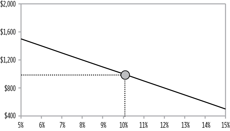
The easiest way to visualize convexity is with an example. Consider a 20.7-year 10% eurobond priced at par. This bond has a modified duration equal to 10. According to duration analysis, if the modified duration equals 10, every time market interest rates change by 1%, the market value of the bond should change by 10%. Since the bond is priced at par, 10% of par is equal to $100. Thus, every 1% change in rates would result in a $100 change in the price of the bond. If this is true, the price/yield relationship of this bond would be as illustrated in Figure 12.1.
FIGURE 12.1
The Price Yield Function of a Bond
However, when we observe the actual relationship between the price and yield of this bond in the market, the relationship looks more like the pattern shown in Figure 12.2. When looked at from below, the actual relationship is not linear. Instead, the price path appears to be convex, hence the name “convexity” (as shown in Figure 12.2).
The first question we need to answer then is, “Why is the price-yield relationship for this bond convex?”
Positive Convexity

The reason is that the value of a .01 ΔIR changes as interest rates change. Initially the value of a .01 ΔIR is equal to:
MV × MD × .0001 = Value .01 ΔIR
$1,000 × 10 × .0001 = $1
However, as interest rates change, both the market value and the modified duration change. For example, as interest rates rise, both the MD and MV decline—lowering the value of a .01 ΔIR.

As interest rates continue to rise, the value of a .01 ΔIR continues to decline and each successive increase in rates results in a smaller loss of MV. Likewise, as market interest rates decline, the modified duration and the value of a .01 ΔIR increase. Thus, as interest rates continue to decline, the resulting increase in the market value becomes progressively greater.
Given the choice between investing in a bond that has a linear price yield relationship or one with a convex price yield relationship, any investor would prefer the bond with the convex path—all other factors being equal. After all, the convex line results in smaller losses and larger gains from symmetric interest rate changes. Since this bond’s price convexity benefits the investor regardless of whether rates rise or fall, this bond exhibits positive convexity in both directions.
All bullet bonds exhibit positive convexity. Their durations extend when rates decline and their durations shorten when rates rise—just what an investor would do when actively managing the portfolio. Of course, not all bonds are bullet bonds, and not all bonds exhibit positive convexity.
For example, consider a pool of current coupon mortgages. When interest rates decline, investors normally want to increase the duration of their portfolios in order to increase their gains. However, as market interest rates decline, an increasing percentage of the homeowners in the pool refinance their mortgages. Refinancing shortens the mortgage pool’s duration. Thus, instead of getting progressively larger gains as interest rates decline, investors in current coupon mortgages get progressively smaller gains as rates decline.
Likewise, when interest rates rise, investors normally try to shorten the duration of their portfolios in order to minimize their losses. However, when rates rise, the duration of a pool of mortgages often extends because fewer people can afford to move up to larger homes or take new jobs that require relocating. Thus the duration of the pool gets longer just when the investor wants it to get shorter.
Since the duration of a pool of mortgage changes in the opposite way investors would choose, pools of current coupon mortgages exhibit negative convexity, as shown in Figure 12.3. (Note that not all mortgage pools exhibit negative convexity—but that current coupon mortgages generally do.)
FIGURE 12.3
Price Yield of Current Coupon Mortgage Pool

Some bonds exhibit positive convexity when rates change in one direction but not when they move in the other direction. Consider the case of a 10-bond that is currently priced at par, is callable at par in 2 years, but matures in 10 years. This bond’s remaining life will either be 2 years or 10 years, depending on whether the bond is called.
As interest rates rise, the probability increases that the bond will last 10 years. As interest rates decline, the probability increases that the bond will only last 2 years. As the projected maturity of the bond changes, so does its projected duration. As interest rates decrease, the bonds expected life and duration decrease, which is the opposite of what the investor would desire. As interest rates rise, the bonds expected life and duration extend—again to the detriment of the investor. Thus, this callable bond exhibits negative convexity along a long portion of the price yield relationship. A callable bond will exhibit positive convexity only if interest rates rise to the point where the embedded option becomes valueless, or rates fall to the point where having the bond called is a virtual certainty.
Clearly, from the investor’s point of view, positive convexity is a very desirable characteristic for an investment to have. Unfortunately, like any other desirable characteristic, such as high credit quality or liquidity, positive convexity has to be purchased. It is purchased by accepting a lower yield from bonds that exhibit positive convexity than from those bonds that exhibit negative convexity. An instrument with positive price convexity will yield less than an instrument with neutral or negative convexity—all other factors being equal.
To perform the type of “what-if” analysis discussed in the last section, it is necessary to calculate a bond’s convexity and then determine how much of an impact the bond’s convexity will have on the bond’s price. The next equation is used to calculate the modified convexity of a bullet bond:

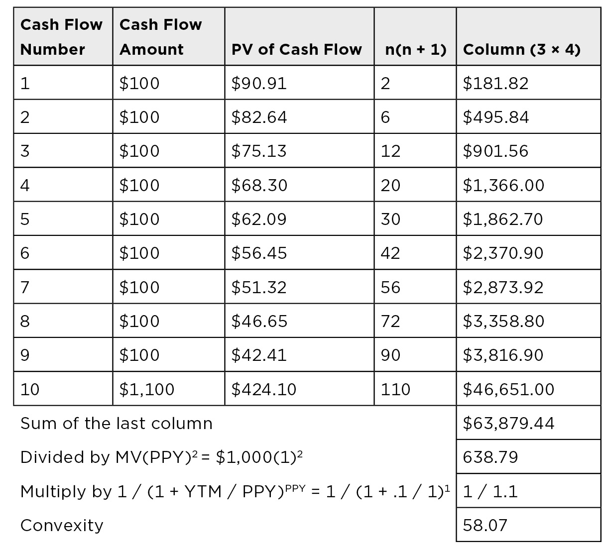
Figure 12.4 illustrates the calculation of the modified convexity of a 10% 10-year eurobond priced at par.
FIGURE 12.4
Calculating Modified Convexity
Once the convexity (C) is calculated, it can be used to calculate the expected price change of a bond due to a change in rates. The formula for the price change expressed as a percentage is:
ΔPrice(%)CONV = [.5 × C × (ΔYTM.)2]
For example, if interest rates were to change by 150 basis points, the value of the 10-year 10% eurobond would change by 0.653% as a result of its convexity.
ΔPrice(%)CONV = [.5 × 58.07 × (.0150)2] = .00653 = 0.653%
Note, that since this is 2nd derivative function, the change in yields is squared. Since it is squared, it makes no difference if interest rates rise or fall since both positive and negative numbers, when squared, are positive numbers. Also, since in the price change calculation above, the yield change is squared, small changes in rates result in almost no convexity impact.
For example, for a 1bp change in rates:
ΔPrice(%)CONV = [.5 × 58.07 × (.0001)2] = .00000029 = 0.000029%
This is less than $.01 in dollar terms. For small changes in market interest rates, the impact of convexity can be safely ignored.
As with duration, the price change due to convexity can also be calculated in dollars by rearranging the equation. The formula for determining the price change of the bond (expressed in dollars) in response to a change in rates as a result of convexity is:
ΔPrice($)CONV = [.5 × MV × C × (ΔYTM.)2]
For the eurobond in our example, the change in price due to convexity in dollars given a 150bp change in yield would be:
ΔPrice($)CONV = [.5 × 58.07 × 1,000 × (.0150)2] = $6.53
The total price change of a bond in response to a change in rates is equal to the sum of the impact of the 1st derivative function (duration) and the 2nd derivative function (convexity).
ΔPrice($)TOTAL = ΔPrice($)DUR + ΔPrice($)CONV
Again using the 10-year 10% eurobond, calculate the change in price due to 100bp change in rates. If rates rise, the change in price due to duration and convexity is:
ΔMVDUR = MV × MD × ΔYTM
ΔMVDUR = $1,000 × –6.15 × .0100 = –$61.50
ΔMVCONV = .5 × MV × C × (ΔYTM)2
ΔMVCONV = .5 × 1,000 × 58.07 × (.0100)2 = $2.90
ΔPrice($)TOTAL = –$61.50 + $2.90 = –$58.60
If rates decline, the total price change would be:
ΔMVDUR = $1,000 × –6.15 × –.0100 = $61.50
ΔMVCONV = .5 × 1,000 × 58.07 × (–.0100)2 = $2.90
ΔPrice($)TOTAL = $61.50 + $2.90 = $64.40
Thus, given a symmetric 100bp change in yields, an investor would profit by $64.40, but only lose $58.60. Since the projected gain exceeds the loss, price convexity benefits the investor.
As another example, calculate the impact of a 100bp change in rates on a 30-year 8% ZCB that pays semiannually.
First calculate the MD. For this bond:
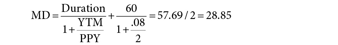
Next, calculate the C. For this bond:

Then calculate the total change in price if interest rates rise and fall by 100 basis points. If rates fall:
ΔPrice($)DUR = $95.06 × 28.85 × (–.0100) = $27.42
ΔPrice($)CONV = .5 × $95.06 × 845.97 × (–.0100)2 = $4.02
ΔPrice($)TOTAL = +$31.44
If rates rise:
ΔPrice($)DUR = $95.06 × 28.85 × (–.0100) = –$27.42
ΔPrice($)CONV = .5 × $95.06 × 845.97 × (–.0100)2 = $4.02
ΔPrice($)TOTAL = –$23.40
The Factors That Impact Convexity
Three basic rules explain how a bond’s characteristics impact its price convexity and how to estimate the relative convexities of different bonds.
- If yield and maturity are held constant, as a bond’s coupon declines its convexity increases.
- If yield and modified duration are held constant, as a bond’s coupon declines, its convexity decreases.
- As maturity increases arithmetically, convexity generally increases exponentially.
Constant Yield and Maturity
If yield and maturity are held constant, as a bond’s coupon declines its convexity increases. Thus, the convexity of a 5-year ZCB priced to offer an 8% YTM will be greater than the convexity of any 5-year coupon bond priced to offer the same return. The lower the coupon, the higher the convexity.
Calculate the price of 30-year euro zero offering yields from 2% to 20%. Graph the result. What is the price of the bond if it offers a 10% return? Suppose an investor thought there was a 50% chance rates would rise by 1% and a 50% chance rates would fall by 1%. What would the bond be worth then?
ANSWER:
Figure 12.5 presents the graphed result of the price calculation of the euro ZCB.
FIGURE 12.5
Zero Coupon Bond Chart Showing Convexity and Pricing Table

At a 10% return, the bond is worth $53.54.
A 50/50 of the 11% and 9% price is ($71.29 + 40.46) / 2 = $55.77.
The bond is worth more when volatility is expected.
Constant Yield and Modified Duration
If yield and modified duration are held constant, as a bond’s coupon declines, its convexity decreases. Thus, the convexity of a 5-year ZCB priced to offer 8% will be lower than the convexity of any other bond with same MD. In order for another bond to have the same MD, it would, of course, have to have a longer life. The wider the dispersion of cash flows, the higher the convexity.
Constant Yield and Coupon
As maturity increases arithmetically, convexity generally increases exponentially. This leads to one of the most common trades: the bullet barbell trade. Consider the graph presented in Figure 12.6. It shows 3 ZCBs: a 2-year, a 4-year, and a 6-year. Since they are ZCBs, the maturities and durations are the same. Suppose you wanted to build a portfolio that had a duration of 4 years.
FIGURE 12.6
Yield vs. Maturity / Duration for ZCBs
There are three ways to do this without taking short positions:

Implementing a Bullet vs. Barbell Trade
- Put 100% into the 4-year ZCB (known as the bullet)
- Put 50% into the 2-year and 50% into the 6-year (known as the barbell)
- Put a third into each (known as the ladder—but note is a combination of the bullet and barbell)
All have durations of 4 years, but which has the highest yield? Figure 12.7 shows the bullet and barbell.
FIGURE 12.7
Bullet vs. Barbell Play

Because the graph shown in Figure 12.7 has some curvature, the bullet offers a higher yield than the barbell. Since the ladder is just the combination of the two, its yield is in between. If the bullet offers a higher return why would anyone want to buy the barbell? The answer is the barbell offers higher convexity and will outperform on a total return basis if interest rate volatility increases, as shown in Figure 12.8.
Bullet-Barbell Trade-Off
|
Portfolio |
Yield |
Convexity |
|
Bullet |
High |
20 |
|
Ladder |
Mod |
20.67 |
|
Barbell |
Low |
24 |
The Higher Derivatives
As we stated earlier, modified duration is the 1st derivative of the price/yield function and convexity is the 2nd derivative of the price/yield function. There is also a 3rd derivative, a 4th derivative, a 5th derivative, and so on. You generally don’t need to consider these because in the 3rd derivative the yield change is cubed, in the 4th derivative the yield change is raised to 4th power, and so forth. Thus, unless the interest rate change is very large, the impact of these functions on the price is minimal.
The only exception is when the size of the cash flows of the security themselves change as interest rates change. For example, the projected cash flows generated by interest-only collateralized mortgage obligations change dramatically as interest rates change. In this case, duration and convexity alone are not enough to describe the behavior of the security, and the higher derivative functions have to be used.