CHAPTER THIRTEEN
Credit Risk
When most people hear the term “credit risk,” they interpret it as the risk that a payment they are owed will be missed, late, or only partially paid—in other words, a default will occur. Defaults are certainly instances of credit risk, but credit risk extends far beyond defaults. Investors can suffer losses on a note even when all the payments are made in full and on time. The losses in this case are indirect and result from the deterioration of credit quality. For example:
- Suppose a bank holds a large quantity of A rated bonds. They are later downgraded to BB+. Even though no payments have been missed the bank may have to hold a larger reserve against the bonds. This reduces the amount the bank can lend and thus reduces the bank’s income.
- Suppose a fixed income mutual fund portfolio manager has purchased a large quantity of A rated bonds that are subsequently downgraded. As they are downgraded, their value declines, which causes the value of the fund’s shares to decline, which causes some current investors to sell and some potential investors to look elsewhere. The value of the fund’s portfolio declines and, because the manager gets a fee based on the assets under management, the manager’s fee declines—despite the fact that every cash flow has been received in full and on time.
- Suppose an insurance company owns some bonds that are downgraded from investment grade to high yield. Regulations may require the company to sell the bonds at a loss even if the company believes the bonds will not default. When the company reinvests the reduced sales proceeds, it will suffer a reduction of cash flow.
- Suppose you sold credit protection on $100MM of Ford Motor company bonds. The bond’s credit quality declines causing the bond’s value to decline to $80MM. Since you sold credit protection, you are marked to the market and must transfer $20MM to the bondholder even though there has been no default. Two years later, the bonds recover, and the $20MM is returned to you. Even though you eventually got your $20MM back, you still lost the interest you could have earned on that $20MM while it temporarily transferred to the protection buyer.
The bottom line is that credit risk is much broader than just default risk.
Working with credit as an investor distills down to two questions:
- What are you paid for assuming credit risk?
- What should you be paid for assuming credit risk?
It’s very simple. If a bond is paying investors 200 basis points for assuming credit risk and 100 basis points is the fair compensation, the bond is a buy! However, if a bond is paying investors 75 basis points for credit risk but 100 basis points is fair compensation, the bond is a sell. Let’s start with looking at how we determine what an investor is being paid for assuming credit risk.
The starting point of this analysis is the total spread. The total spread is the yield spread between the bond and the equivalent risk-free investment(s). For example, suppose a 10-year risk-free T-note yields 8%, and a 10-year risky investment yields 10%. The spread is 2% or 200 basis points.
The spread can be quoted to the US Treasury or the fixed side of an interest rate swap with the same maturity or the same duration. The spread can also be to the Treasury or the swap zero coupon curves.
Regardless of which you use as the base rate for defining the spread, many investors refer to the total spread as the credit spread. That is not correct. The total spread compensates the investor for at least eight other risks in addition to default risk. These risks include:
- Tax risk
- Tax increase risk
- Liquidity risk
- Cost of analysis risk
- Credit drift risk
- Credit convexity risk
- Uncertainty risk
- Embedded option risk
Only after subtracting the fair compensation for the other five risks from the total spread can we determine what the investor is receiving for credit risk. Let’s look at each of these risks in turn.
TAX RISK
For an investor who is subject to taxes, the goal is to maximize the after-tax return. In the United States, the interest received from risk-free Treasuries is only subject to federal income tax, while the interest received from risky corporate bonds is subject to federal, state, and city income taxes. Given tax rates of 35% federal, 6% state, and 4% city and assuming that federal taxes are deductible at the state level and both federal and state are deductible at the city level, the after-tax incomes are:
Treasury = 8% × (1 − .35) = 5.2%
Corporate = 10% × (1 − .35) = 6.5% × (1 − .06) = 6.11% × (1 − .04) = 5.87%
Taxes reduce the spread for the remaining risks from 200 basis points to 67 basis points (5.87% to 5.2%). This is not the entire tax impact.
TAX RATE INCREASE
If, in the future, the state and/or city tax rates increase, the spread between the two returns would narrow even further. Investors considering investing in a risky asset must be sure that they receive adequate compensation—not just for the impact of taxes today, but also for the impact of potentially higher tax rate rates in the future. Also, if either bond is purchased at a discount, the differential between the income and capital gains tax rates will also impact the after-tax spread.
The important point is that since everyone’s tax rates and assumptions regarding future tax rates are going to be different, so will everyone’s after-tax credit spread. The spreads on Bloomberg, the WSJ, and the evening news usually assume zero taxes and are grossly incorrect for the vast majority of investors.
LIQUIDITY
The only advantage to the United States being more than $17 trillion in debt is that the US Treasury market is remarkably liquid. If a security is liquid, it can be bought or sold:
- Quickly
- At a fair price
- With no or minimal market impact
You can buy or sell $100MM in Treasuries immediately, at fair value, and not have your trade move the market—not so with most corporate bonds. While there are a few liquid corporate bonds (usually issued by America’s largest companies), the vast majority of corporate bonds are significantly less liquid. This means the dealer’s bid-ask spreads are wider to compensate. Also, when you buy or sell, you can end up competing against yourself because your transaction alone moves the market.
For example, you want to by $50MM of the 8% XYZs of Aug 15, 2032. The current best bid and offer is 102 by 103. As you buy the bonds—starting at 103—your buy causes the price to rise, so your order is completed as follows:
$10MM at 103
$10MM at 103⅛
$10MM at 103⅜
$10MM at 103½
Thus, your average price was 103¼. Now, however, the bid ask spread is 102½ by 103½, so the price has to rise by ¾ of a point just to break even.
Different investors place different value on liquidity. An investor who buys and holds to maturity is less interested in liquidity than a portfolio manager who actively trades. To price liquidity, each investor has to solve the following equation for his own circumstances:
Price of liquidity = Probability of sale × Estimated costs of selling
Thus, an investor who thought liquidity would cost 100 basis points but who also thought there was a 5% chance of sale would put the cost of liquidity at 5 basis points. This reduces the total spread by another 5 basis points.
COST OF ANALYSIS
Managing a portfolio of US Treasuries requires only macroeconomic research. How will the yield curve shift? What will the inflation rate be? What actions, if any, will the Fed take? Since the US government can print money, there’s no need for microeconomic credit analysis. However, when managers add corporate bonds to their portfolios, they almost always incur additional expenses, including the cost of:
- Subscribing to Moody’s and Standard & Poor’s credit services
- Adding credit analysts (salaries, office space, technology, and the like)
- Upgrading their trustee relationship to allow for corporate events (takeovers, bond conversions, and the like)
All of these additional costs have to be paid from the spread because they are only necessary for owners/managers of corporate bonds. The impact on the spread will depend on the additional costs incurred as well as the size of the corporate bond portfolio. If these costs total $1MM a year and the portfolio is a $1 billion portfolio, then 10 basis points of the spread just pays for the cost of analysis.
CREDIT DRIFT RISK
If an investor with $100MM to invest was to select 100 Baa rated bonds, invest $1MM in each one, and hold them over time, some of the bonds would experience credit upgrades and some of the bonds would experience downgrades. Over time, however, the investor will experience more downgrades than upgrades. It doesn’t matter if the economy is weak, normal, or strong; there are always more downgrades than upgrades. Figure 13.1 depicts the credit drift for industrial bonds over a 5-year period.
Credit Drift

Looking at the BBB bonds, only 81% still have a BBB bond rating after 5 years. The number of full downgrades to BB is almost three times the number of full upgrades to A. The number of double downgrades is more than 30 times the number of double upgrades.
The reason why there are more downgrades than upgrades is that once a company borrows the money it needs, management doesn’t care about the bondholders. Management is elected by the shareholders, and management’s number one goal is to reward shareholders. Many of the actions that management takes to reward shareholders can penalize bondholders, including raising dividends and buying back shares.
CREDIT CONVEXITY RISK
Even if an investor was so good at selecting bonds that the portfolio experienced the same number of upgrades and downgrades, the value of a portfolio will still decline over time. The reason for this is that a bond’s price declines more on a downgrade than it rises on an upgrade. There is a larger change in yield in a downgrade than an upgrade. In Figure 13.2, the baseline is the yield of the US Treasury. As the credit quality declines, the incremental spreads increase by an ever-increasing amount.
FIGURE 13.2
Credit Convexity

UNCERTAINTY PREMIUM
The cost of credit default risk is equal to the:
Amount at risk × the probability of default × the percentage lost in default
At least two of those variables can only be estimated. This introduces a source of uncertainty in the arbitrage relationship between risk-free and risky investments. Suppose that a risk-free bond portfolio yields 8% and that a risky portfolio of corporates is expected to yield 8% after all defaults and delays. Because the corporate bond return can only be estimated, many managers demand that the expected return of the corporate portfolio exceed the return from the risk-free portfolio before they consider it to be equal. Thus, a manager might require that the expected return on the corporate portfolio exceed the risk-free portfolio by 10 basis points before considering them to be “equally” attractive. Each manager and investor sets their own uncertainty spread.
EMBEDDED OPTIONS
If a bond is callable, the investor has sold the issuer the right to redeem the bond early. The issuer will call the bond if rates decline and the company can issue new debt at a lower rate. Of course, this forces the investor to reinvest at a lower rate—lowering the investor’s RCY, NRCY, or NNRCY. The premium the investor receives for selling this option is incorporated into a higher spread. To illustrate this process, we’ll look at two embedded option pricing models: an admittedly oversimplified model that just illustrates the concept and the Bloomberg Single Factor Option-Adjusted Spread (OAS) Model.
Simplified Embedded Option Pricing Model
In this model, we’re going to build a price tree and use that tree to value the bond under the assumption that there are no options. Then, we’re going to adjust the price tree for an option and value the bond again. When we add an option to the tree, we will get a lower value for the bond. Since the only change we made was to add the impact of an option, the difference in the values must equal the value of the option. To illustrate, let’s start with a note that is currently selling at $1,010 and is callable for the next 4 months at a price of $1,020. To keep the model simple, we’ll build a binomial tree. Since the note has experienced an average price change of $10 per month and there is a 50/50 chance that interest rates will increase or decrease each month, the tree would be as shown in Figure 13.3.
FIGURE 13.3
Binomial Tree
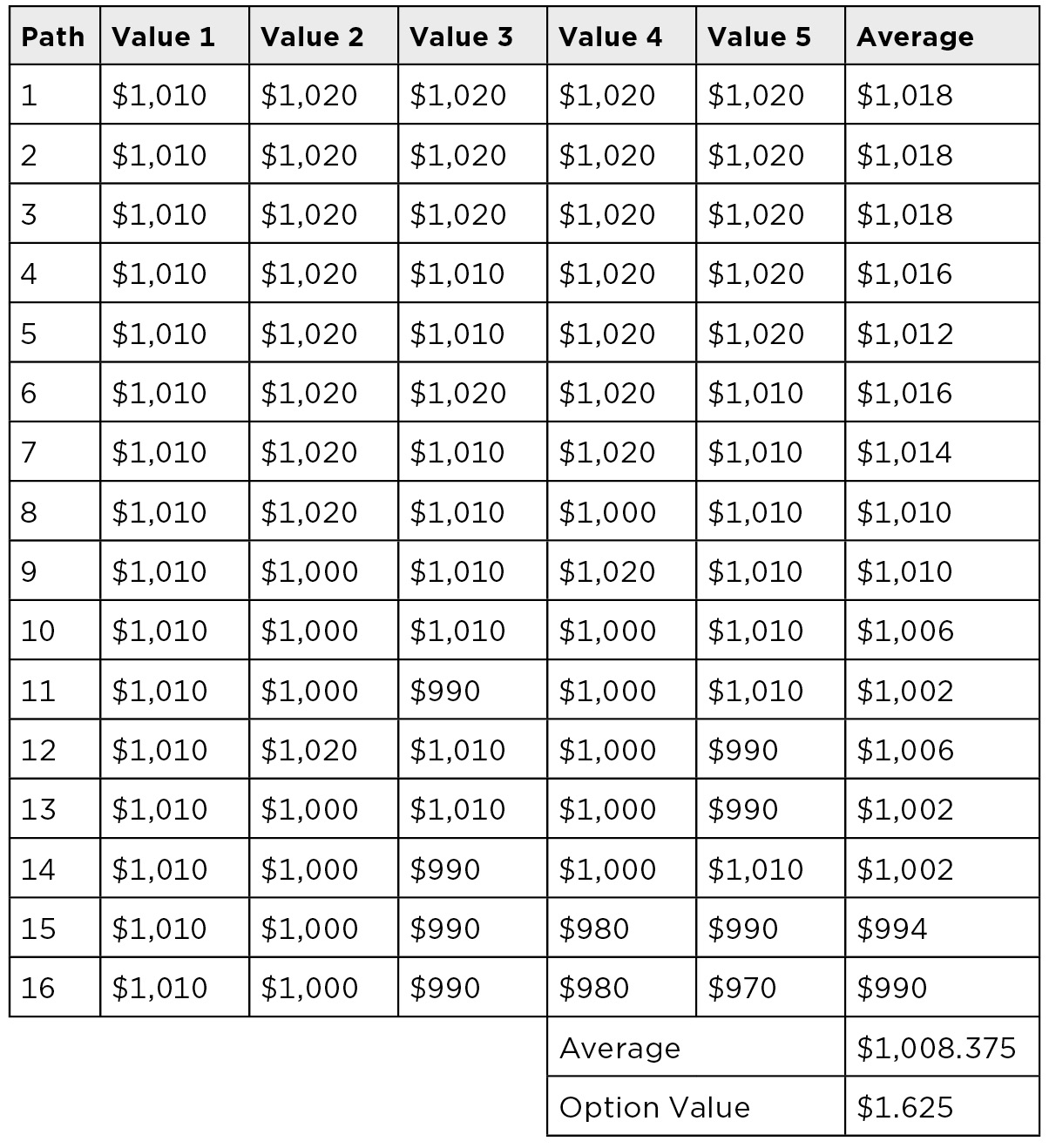
Now, if starting at $1,010, we flip a coin, it comes up heads, and the price goes up. We flip again, it comes up tails, and the price goes down. We continue flipping with the results being noted in the path through the tree shown in Figure 13.4. Since we don’t know where along this path the investor will sell the bond, we calculate the average price along the path. Clearly the average price along this path is $1,010. Some of the paths would have higher average prices. Some paths would have lower average prices. But, if you ran thousands of random paths through this tree, the average of the averages would be very close to $1,010.
FIGURE 13.4
Random Path from Tree

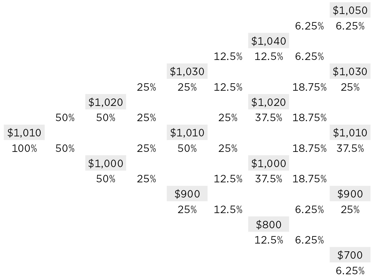
Now, let’s add the call option that allows the issuer to call the bond at $1,020. Adding this option effectively caps the note at $1,020. (Even if the bond is not called, the fact that the bond can be called at $1,020 will prevent anyone from paying more than $1,020 for the bond.) This reduces the average price along the paths along the top of the tree (as shown in Figure 13.5) and the amount the investor can expect from investing in this bond. The average price along the paths drops to $1,008.375 from $1,010.00.
FIGURE 13.5
Lower All Values Higher Than $1,020

Adding the option reduces the investor’s expected return by $1.625, so if the option is added the investor needs to either receive $1.625 upfront—or a higher yield that has a present value of $1.625. If 12 basis points per year had a present value of $1.625, then 12 basis points of the spread would just pay the investor for the option the investor sold to the issuer. Figure 13.6 shows the paths after adding the call option.
Paths After Adding Option
So after allowing for the value of the other components of the spread, the actual spread for credit risk is 30 basis points—not 200 basis points, as depicted in Figure 13.7.
True Compensation for Default Risk After Cost of Other Risks Is Subtracted
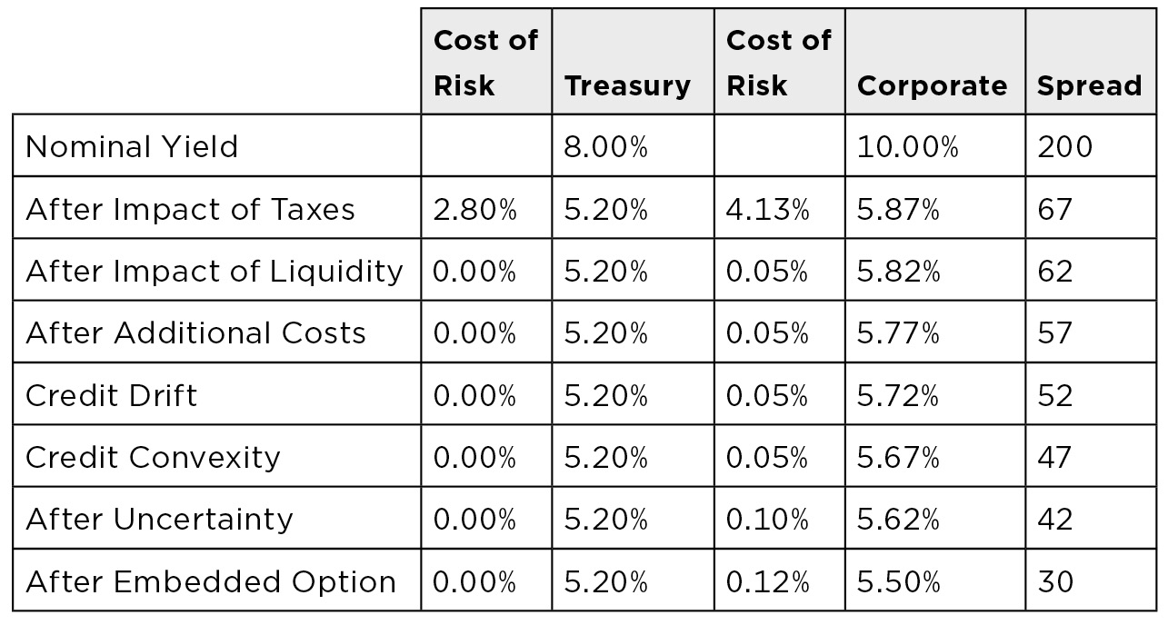
Thus, while the total spread is 200 basis points, the actual compensation for credit risk is just 30 basis points. This is the spread that should be used for relative value analysis. This answers the question “What are you getting paid for taking credit risk?”
BLOOMBERG OAS MODEL
The Bloomberg OAS model is used to estimate the value of embedded options. The model uses a binomial rate tree, as opposed to the price tree used in the simplified model we just reviewed. It is calibrated off the Interest Rate Swap curve instead of the US Treasury curve for two reasons:
- Treasuries are not priced at par. This causes a distortion in the creation of the spot curve and the forward curve. New swaps are priced at par which allows less distortive spot and forward curves to be derived.
- Interest rate swaps have less basis risk. In a political/economic crisis, there is often a flight to quality. This means Treasury yields decline while all other yields rise. Since embedded options are found in corporate bonds, which almost never have an AAA rating, their value should move with lower quality instruments—not Treasuries.
In this model, it is assumed that future interest rates are distributed around the forward swap curve, and that the width of the distributions is based solely on the current volatility of short-term rates. Because the width of the distribution is based solely on the current volatility of short-term rates, this model is often referred to as the “Bloomberg single factor model.”
Building the Tree
From the current IRS swap rates, calculate the zero coupon swap rates. From the zero coupon rates, calculate the forward swap rates.
For example, if the spot swap rates are:
- 1-year swap = 7%
- 2-year swap = 7.4988%
- 3-year swap = 7.9969%
Then the forward interest rate swap rates, as shown in Figure 13.8, are:
- 1-year swap = 7%
- 1-year swap in 1 year = 8% = {[(1 + .074988)2] / [1 + .071]} − 1
- 1-year swap in 2 years = 9% = {[(1 + .079968)3] / [(1 + .074988)2]} − 1
Once the forward rates are determined, the width of the distribution of possible rates around the 1-year rate in 1 year can be determined using the formulas shown in Figure 13.9 and Figure 13.10.
FIGURE 13.8
Possible Distribution of Rates
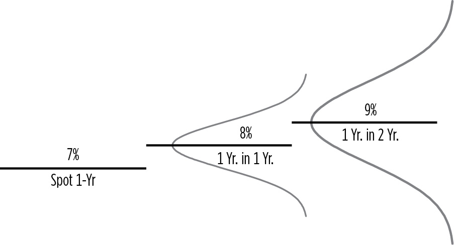
FIGURE 13.9
1-Year Rate in 1 Year, Formula 1
(Probability of rates declining × Weighted average of the lower rates) + (Probability of rates rising × Weighted average of the higher rates)
Normally, we assume a 50/50 chance of rates rising vs. falling.
1-Year Rate in 1 Year, Formula 2
Q = Weighted average (by probability) of rates above the Implied Forward Rate / Weighted average (by probability) of rates below the Implied Forward Rate
Q = e2σSqrt(t)
Weighted average high rates = Q × Weighted average low rates
If the volatility of short-term rates is 15%, then
Q = e2(.15)sqrt(1) = 1.35
.5(weighted average of higher rates) + .5(weighted average of lower rates) = 8%
This second equation has two variables, and thus it has an infinite number of solutions. However, we know the weighted average of higher rates is 1.35 times the weighted average of lower rates, thus this second equation (shown in Figure 13.11) becomes:
.5(1.35 × weighted average of lower rates) + .5(weighted average of lower rates) = 8%
1.175 (weighted average of lower rates) = 8%
Low rate = 6.81%
High rate = 1.35 × 6.81 = 9.19%
Verify .5(9.19) + .5(6.81) = 8%
Building a Binomial Rate Tree for the Bloomberg Single Factor OAS Model
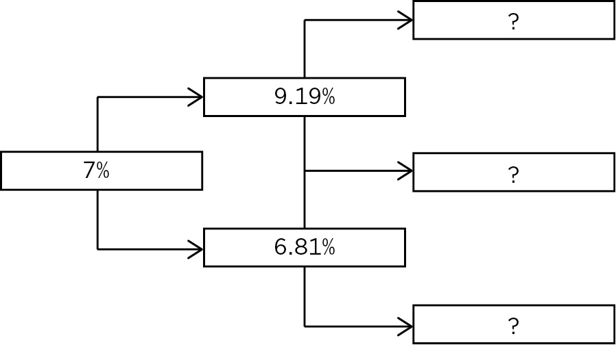
At the next (third) step of the tree, the probabilities and weighted average are:
.25(High rate) + .50(Middle rate) + .25(Low rate) = 9% (1-year rate in 2 years)
Restating the three variables in terms of one variable results in the following, which is shown graphically in Figure 13.12:
.25(1.352 Low rate) + .50(1.35 Low rate) + .25(Low rate) = 9%
1.38(Low rate) = 9%
Low rate = 6.52%
Middle rate = (6.52% × 1.35) = 8.8%
High rate = (8.8% × 1.35) = 11.88%
Restating the Three Variables in Terms of One Variable

This process would be repeated, going out for up to 30 years.
Once the tree is created it, can be used to:
- Value AA rated bullet bonds assuming a volatile rate environment
- Value AA rated bonds with embedded options
- Value bonds with other credit ratings
It is a very versatile and powerful tool as we shall see below, starting by using the tree to calculate the impact of volatility on price.
IMPACT OF VOLATILITY ON PRICE
A bond has a different value in a volatile as opposed to a nonvolatile interest rate environment. To illustrate, let’s value a 9% 3-year eurobond. Let’s first value it assuming zero volatility, in which case the bond is equal to the present value of its future cash flows as depicted in Figure 13.13.
FIGURE 13.13
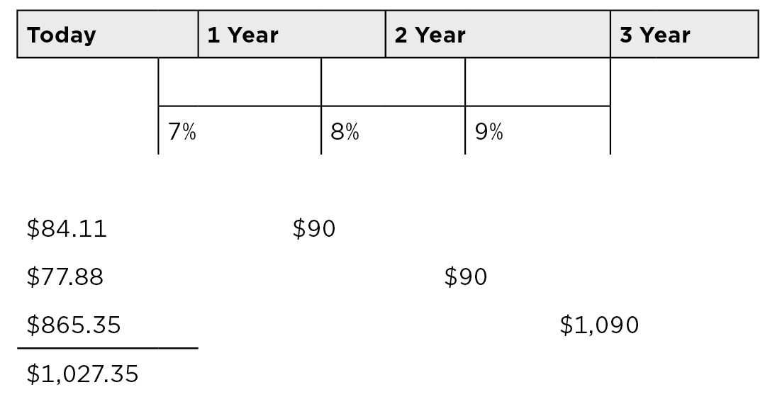
Now, let’s value the bond using the tree. There are four paths through this tree, each of which has a 25% of occurring. The bond’s cash flows have to be present valued four different ways:
If rates rise twice, then the value = $1,090 / (1.1188) / (1.0919) / (1.07) + $90 / (1.0919) / (1.07) + $90 / (1.07) = $995.03
If rates rise then fall, then the value = $1,090 / (1.088) / (1.0919) / (1.07) + $90 / (1.0919) / (1.07) + $90 / (1.07) = $1,018.63
If rates fall then rise, then the value = $1,090 / (1.088) / (1.0681) / (1.07) + $90 / (1.0681) / (1.07) + $90 / (1.07) = $1,039.47
If rates fall twice, then the value = $1,090 / (1.0652) / (1.0681) / (1.07) + $90 / (1.0681) / (1.07) + $90 / (1.07) = $1,058.24
Average = $1,027.84
When valued using the tree (incorporating volatility), this simple three cash flow note is worth an extra ($1,027.84 − $1,027.35) = $0.49. This is not the result of any rounding error. The reason for the discrepancy is that in a volatile environment, the price is expected to change and the bond’s convexity (see Chapter 12) causes larger gains and smaller losses. Unless an investor expects interest rates to have no volatility, $1,027.84 is the more accurate valuation.
VALUING EMBEDDED OPTIONS
To value the embedded options, first work the cash flows back through the tree, as shown in Figure 13.14.
FIGURE 13.14
Value by Walking Back Through the Tree

Sample calculation: {[.5 × ($1,090 / 1.1188) + .5 × ($1,090 / 1.1188)] + $90 payment} = $1,064.26
Thus, the price of the bond is $1,027.84. Now, suppose the bond is callable at par. In this case, every value above $1,090 has to be lowered to $1,090 as shown in Figure 13.15. This lowers the present value from $1,027.84 to $1,012.76, a difference of $15.08. The value of the option, therefore, is $15.08. This would have to be converted into a yield spread that had an equivalent PV.
FIGURE 13.15
Bond Callable at Par Alternative

BONDS WITH DIFFERENT RATINGS
The original swaps that were used to create the yield tree were AA rated, and so the rates that result are appropriate only for AA rated bonds. If the bond has a different rating, a spread has to be added to each of the rates to account for the credit risk. Given the spread, the bond can be priced. If the bond already has a price, investors can work backwards to determine what spread needs to be added.